Modélisation de la croissance des plantes supérieures pour les systèmes de support-vie : conception d'un modèle global et simulation des transferts de masse et d'énergie à l'échelle de la plante

(1)

HAL Id: tel-01935086

https://tel.archives-ouvertes.fr/tel-01935086

Submitted on 26 Nov 2018

HAL is a multi-disciplinary open access

archive for the deposit and dissemination of sci-entific research documents, whether they are pub-lished or not. The documents may come from teaching and research institutions in France or abroad, or from public or private research centers.

L’archive ouverte pluridisciplinaire HAL, est destinée au dépôt et à la diffusion de documents scientifiques de niveau recherche, publiés ou non, émanant des établissements d’enseignement et de recherche français ou étrangers, des laboratoires publics ou privés.

global model design and simulation of mass and energy

transfers at the plant level

Pauline Hezard

To cite this version:

Pauline Hezard. Higher plant growth modelling for life support systems : global model design and sim-ulation of mass and energy transfers at the plant level. Chemical and Process Engineering. Université Blaise Pascal - Clermont-Ferrand II, 2012. English. �NNT : 2012CLF22250�. �tel-01935086�

(2)

N° DU : 2250 Année 2012

Ecole Doctorale

Sciences de la Vie, Santé, Agronomie, Environnement

Numéro d’ordre : 583

Thèse

Présentée à l’Université Blaise Pascal Pour l’obtention du grade de

D

O

C

T

E

U

R

D

’

U

N

I

V

E

R

S

I

T

E

Spécialité

Génie des Procédés

Soutenue le 12 septembre 2012 par

Pauline HEZARD

Modélisation de la croissance des plantes supérieures pour les

systèmes de support-vie : conception d’un modèle global et

simulation des transferts de masse et d’énergie à l’échelle de la plante

Devant le jury composé de :

Président du jury : M. LARROCHE Christian, Professeur, Université Blaise Pascal, Clermont-Ferrand

Examinateurs : M. MERGEAY Max, DR, SCK-CEN, Mol, Belgique

Mme PAILLE Christel, Ingénieur, ESA-ESTEC, Noordwijk, Pays-Bas

Rapporteurs : M. COURNEDE Paul-Henry, Professeur, Ecole Centrale des Arts et Manufactures de Paris, Châtenay-Malabry

M. LEGRAND Jack, Professeur, Université de Nantes, Saint-Nazaire

Directeur de thèse : M. DUSSAP Claude-Gilles, Professeur, Université Blaise Pascal, Clermont-Ferrand

Institut Pascal, axe Génie des Procédés, Energétique et Biosystèmes –

Université Blaise Pascal – CNRS UMR 6602

(3)

(4)

N° DU : 2250 Année 2012

Doctoral school of

Life Sciences, Health, Agronomy, Environment

Order Number: 583

Thesis

Submitted to the University Blaise Pascal For the the award of the degree of

D

o

c

t

o

r

o

f

P

h

i

l

o

s

o

p

h

y

Specialty:

Process Engineering

Presented the 12th September 2012 by

Pauline HEZARD

Higher Plant Growth Modelling for Life Support Systems:

Global Model Design and Simulation of Mass and Energy

Transfers at the Plant Level

For the jury composed of:

President: Mr LARROCHE Christian, Professor, Université Blaise Pascal, Clermont-Ferrand, France

Examiners: Mr COURNEDE Paul-Henry, Professor, Ecole Centrale des Arts et Manufactures de Paris, Châtenay-Malabry, France

Mr LEGRAND Jack, Professor, Université de Nantes, Saint-Nazaire, France

Mr MERGEAY Max, Director of Research, SCK-CEN, Mol, Belgium

Mrs PAILLE Christel, Engineer, ESA-ESTEC, Noordwijk, Netherlands

Thesis director: Mr DUSSAP Claude-Gilles, Professor, Université Blaise Pascal, Clermont-Ferrand, France

Institut Pascal, axe Génie des Procédés, Energétique et Biosystèmes –

Université Blaise Pascal – CNRS UMR 6602 – France

(5)

(6)

Les missions spatiales habitées de longue durée nécessitent des systèmes de support-vie efficaces recyclant l’air, l’eau et la nourriture avec un apport extérieur minimum en matière et énergie. L’air et l’eau peuvent être recyclés par des méthodes purement physico-chimiques, tandis que la production de nourriture ne peut être faite sans la présence d’organismes vivants. Le projet Micro-Ecological Life Support System Alternative (MELiSSA, alternative de système de support-vie micro-écologique) de l’Agence Spatiale Européenne inclut des plantes supérieures cultivées dans une chambre close contrôlée, associée à d’autres compartiments microbiens. Le contrôle à long terme de la chambre de culture et du système de support-vie entier requiert des modèles prédictifs efficaces. Le bouclage du bilan massique et la prédiction de la réponse de la plante dans un environnement extraterrestre inhabituel mettent en avant l’importance de modèles mécanistes basés sur le principe des bilans de matière et d’énergie. Une étude bibliographique poussée a été réalisée afin de lister et analyser les modèles de croissance de plantes supérieures existants. De nombreux modèles existent, ils simulent la plupart des processus de la plante. Cependant aucun des modèles structurés globaux n’est suffisamment mécaniste ni équilibré en terme d’échange de masse pour une application dans un système de support-vie clos. Ainsi, une nouvelle structure est proposée afin de simuler tous les termes du bilan massique au niveau de la plante, en incluant les différentes échelles de l’étude : les processus généraux, l’échelle de l’organe et l’échelle de la molécule. Les résultats d’une première approche utilisant des lois physiques mécanistes simples pour les échanges de matière et d’énergie, une stoechiométrie unique pour la production de biomasse et quelques lois empiriques pour la prédiction des paramètres architecturaux sont illustrés et comparés avec des résultats expérimentaux obtenus dans un environnement contrôlé. Une analyse mathématique du modèle est réalisée et tous ces résultats sont discutés afin de proposer les prochaines étapes de développement. Ceci est décrit en détail pour l’inclusion de modèles de processus plus complexes dans les futures versions du modèle ; les expériences qui devraient être réalisées ainsi que les mesures nécessaires sont proposées. Ceci conduit à la description d’une nouvelle conception de chambre de culture expérimentale.

Mots-clés : modélisation des plantes supérieures; environnement contrôlé;

système de support-vie clos; bilans matière et énergie; phénomènes de transport;

modèle métabolique structuré

(7)

For long-term manned space missions, it is necessary to develop efficient life support systems recycling air, water and food with a minimum supply of matter and energy. Air and water can be recycled from purely physico-chemical systems; however food requires se presence of living organisms. The Micro-Ecological Life Support System Alternative (MELiSSA) project of the European Space Agency includes higher plants grown in a closed and controlled chamber associated with other microbial compartments. The long-term control of the growth chamber and entire life support system requires efficient predictive models. The mass balance closure and the prediction in uncommon extraterrestrial environments highlight the importance of mechanistic models based on the mass and energy balances principles.

An extensive bibliographic study has been performed in order to list and analyse the existing models of higher plant growth. Many models already exist, simulating most of the plant processes. However none of the global, structured models is sufficiently mechanistic and balanced in terms of matter exchange for an application in closed life support systems. Then a new structure is proposed in order to simulate all the terms of the mass balance at the plant level, including the different scales of study: general processes, organ scale and molecular scale. The results of the first approach using simple mechanistic physical laws for mass and energy exchange, a unique stoichiometry for biomass production and few empirical laws for the prediction of architectural parameters are illustrated and compared with experimental results obtained in a controlled environment. A mathematical analysis of the model is performed and all these results are discussed in order to propose further developments. This is described in detail for the implementation of more complex models of processes in the future model versions; the experiments that should be performed including the main measurements are proposed. This leads to the description of a new design of experimental growth chamber.

Key words: higher plant modelling; controlled environment; closed life support

system; mass and energy balances; transport phenomena; structured metabolic

model

(8)

Acknowledgements

Avant tout je tiens à remercier mon directeur de thèse le professeur Claude-Gilles Dussap, qui m’a permis de donner le meilleur de moi-même dans ce sujet passionnant. La liberté qu’il m’a laissée, tout en me guidant, en étant présent et à l’écoute lorsque c’était nécessaire, m’ont énormément appris.

Le docteur Catherine Creuly m’a ouvert la porte à cette aventure, en me proposant une piste alors inattendue dans mon parcours, et m’a aussi soutenue durant toutes mes recherches. Je ne regretterai jamais cette voie et la remercie du fond du cœur.

This work was supported by the European Space Agency through the Micro-Ecological Life Support System Alternative (MELiSSA) project. I am grateful to the head of MELiSSA team and all the partner laboratories working on this subject. The long collaboration of passionate scientists made an enthousiastic working environment. I express my special gratitude to Max Mergeay, the last of the original founders still working in the project, an incredibly smart and kind scientist; Christophe Lasseur, leading this team with all his humour and conviction and Christel Paillé, for her daily presence and great management skills in the case of the huge food characterization project. The experiments and technical knowledge of Mikael Dixon and his team provided me the primary source of data I could work with.

Mes rapporteurs les professeurs Paul-Henry Cournède et Jack Legrand et les membres de mon jury Max Mergeay, Christel Paillé, Claude-Gilles Dussap et Christian Laroche, bien que très occupés, ont pu organiser une première date de soutenance malgré le délai court, puis ont accepté de la reporter au dernier moment. Leur attention et leur gentillesse lorsque ma santé était affaiblie m’ont extrêmement touchée. Je les remercie pour leur attention lors de ma soutenance et pour les remarques pertinentes et questions intéressantes qu’ils m’ont adressées. Ma soutenance reste le meilleur souvenir de tout ce parcours, pourtant riche en moments agréables.

En effet, toute cette aventure n’aurait pas pu être menée à bien sans mes collègues et amis de tous les jours, en premier Swathy, qui a suivi une voie parallèle de la mienne et a influencé mon travail comme ma vie personnelle tout au long de ce travail de longue haleine. Alain m’a soutenue pour la partie la plus difficile et la plus stressante, sans faiblir malgré sa charge de travail, et sans lui le résultat n’aurait pas été du même niveau. Les collègues titulaires ou de long terme au laboratoire, en particulier Béatrice, David, Frédéric, Laurent, Céline,

(9)

Christian m’ont apportés leurs conseils, leurs connaissances et leur bonne entente au quotidien. Tous les doctorants, post-doctorants et stagiaires ont donné la bonne humeur et l’amitié dans ma vie du laboratoire. Un grand merci à Swathy, Alain, Erell, Nele, Stéphanie, Denis, Darine, Akhilesh, Marie-Agnès, Kaies, Cindie, Aurore, Numidia, Oumar, Anil, Reeta, Matthieu, Azin, Jérémy, et tous ceux dont j’oublie le nom mais qui ont apporté des rires dans les bureaux et de bons plats aux repas du mercredi.

Enfin, ma famille et mes amis m’ont aidée tout au long de ces années, je remercie en premier lieu mes parents, ma sœur Marion, mon frère Antoine, ma demie-sœur Maud pour leur présence et leur écoute tout au long de cette aventure. Ma vie internationale Clermontoise grâce à WorldTop, en particulier grâce à Bernard, Mehdi, Hui, LiLi, Changjie, Dallana, Wenbin, Anicet, Ismaël, Francesca, Juan Luis, Yu, Cléo et tous les amis du monde entier, a été une magnifique ouverture d’esprit, très complémentaire de mon travail de thèse. Les discussions passionnées avec Akmal, les rires avec Petra, Priscilla, Ke Hui ; les retrouvailles avec mes amies d’enfance Anaïs, Emilie, Marlène ; les visites de Muriel ou Mélanie, les voyages pour retrouver les cousins, les anciens amis et visiter les régions ou pays que je ne connaissais pas… Toutes ces occasions de changer d’air ont égaillé ma vie quotidienne et ont donné l’allant nécessaire à mes recherches.

Toutes les personnes citées plus haut et toutes celles que j’ai oubliées ont contribué, de près ou de loin, à la réussite de ce travail et à ce que je suis devenue aujourd’hui. Je les remercie du fond du cœur.

(10)

List of Figures

Figure A: In silico representation of the metabolic network including the mass balance

description. ... xxvi

Figure B: Comparison of plant and aimed model structures describing the flows of matter, energy and information. ... xxvii

Figure 1: MELiSSA loop design highlighting the higher plant compartment IVB. ... 2

Figure 1: Comparison of leaf appearance stage (L.A.S.) plotted versus time (days, a.) and versus thermal time (°C day, b.) for winter wheat. ... 12

Figure 2: Plant architectural growth modelling using L-system. ... 14

Figure 3: Water flow driving forces through higher plant from the soil to the atmosphere. ... 27

Figure 4: Aimed model scheme for a simple and mechanistic simulation of plant growth. .... 43

Figure 5: Comparison of plant and model structures describing the flows of matter, energy and information. ... 45

Figure 2.1: Representation of the carbon mass balance taking into account the chamber leakage. ... 64

Figure 2.2: Leakage test showing the reduction in chamber CO2 content with time. ... 65

Figure 2.3: Comparison of total carbon uptake and oxygen release, taking into account the leakage. ... 69

Figure 2.4: Water dynamics and water balance in higher plants... 70

Figure 2.5: Experimental root water absorption rate of one lettuce. ... 72

Figure 2.6: Experimental uptake rates of one lettuce for nitrogen (N), potassium (K) and phosphorus (P). ... 73

Figure 2.7: Experimental day and night condensation rates, evaluated for one lettuce. ... 74

Figure 2.8: Experimental day photosynthesis rate of one lettuce. ... 76

Figure 2.9: Experimental respiration rate of one lettuce. ... 76

Figure 2.10: Oxygen exchange dynamics of one plant, taking into account the leakage. ... 78

Figure 2.11: Model structure and selected equations. ... 81

Figure 2.12: Comparison of experimental and simulated lettuce growth. ... 91

Figure 2.13: Comparison of experimental and simulated water uptake rate. ... 93

Figure 2.14: Comparison of experimental and simulated carbon exchange rate. ... 94

Figure 2.15: Comparison of experimental and simulated carbon accumulation in biomass. ... 95

Figure 2.16: Simulated light interception, for maximum flux and after limitation. ... 96

Figure 2.17: Comparison of experimental and simulated carbon exchange rates including light limitation. ... 97

Figure 2.18: PyGMAlion software scheme. ... 109

Figure 2.19: Simplified MELiSSA_Plant model structure in PyGMAlion analysis platform. ... 112

Figure 2.20: Model output uncertainty for architectural (a), physical (b) and stoichiometric (c) parameters. ... 114

Figure 2.21: Model output uncertainty for light interception (a), carbon exchange (b), transpiration (c) and water uptake (d) parameters. ... 115

Figure 2.22: Model output linearity for architectural (a), physical (b) and stoichiometric (c) parameters. ... 117

Figure 2.23: Model output linearity for light interception (a), carbon exchange (b), transpiration (c) and water uptake (d) parameters. ... 118

Figure 2.24: Architectural parameters first order sensitivity indices, for biomass (a) and exchange rates (b) outputs. ... 119

(15)

Figure 2.25: Architectural parameters second order sensitivity indices, for biomass (a) and

exchange rates (b) outputs. ... 120

Figure 2.26: Physical parameters first order sensitivity indices, for biomass (a) and exchange rates (b) outputs. ... 121

Figure 2.27: Physical parameters second order sensitivity indices, for biomass (a) and exchange rates (b) outputs. ... 122

Figure 2.28: Stoichiometric parameters first order sensitivity indices, for biomass (a), respiration (b), carbon uptake (c) and water uptake (d) outputs. ... 123

Figure 2.29: Stoichiometric parameters second order sensitivity indices for water uptake output. ... 124

Figure 2.30: Light interception parameters first (a, b) and second order (c, d) sensitivity indices, for biomass (a, c) and exchange rates (b, d) outputs. ... 125

Figure 2.31: Carbon exchange parameters first order sensitivity indices, for biomass (a), respiration (b), carbon uptake (c) and water uptake (d) outputs. ... 126

Figure 2.32: Carbon exchange parameters second order sensitivity for carbon uptake output. ... 127

Figure 2.33: Transpiration rate parameters first order sensitivity indices, for biomass (a), carbon exchange (b) and water uptake (c) outputs. ... 128

Figure 2.34: Water uptake rate parameters first order sensitivity indices, for biomass (a), carbon exchange (b) and water uptake (c) outputs. ... 129

Figure 2.35: Scheme of the model behaviour depending on the limiting rate, pointing out the key parameters. ... 131

Figure 3.1: Young plant specific growth chamber. ... 165

Figure 3.2: Design of a large plant growth chamber permitting sampling without disturbance and separated root and shoot mass balances. ... 167

Figure 3.3: Top view of a part of the growth chamber with air lock system and separation for sampling without disturbing the rest of the canopy. ... 168

Figure 3.4: Sectional views with the detail of the chamber’s air circulation, sample separation and system for holding the plants. ... 169

Figure 3.5: General overview of a high-throughput plant growth experimental system. ... 171

Figure 3.6: Front view scheme of an individual chamber of the high-throughput system with air and solution management. ... 172

Figure 3.7: Overview of the measurement and control systems. ... 173

Figure A 1.1: Theoretical pressure in the chamber, comparison between experimental raw data and data corrected for leakage for oxygen, and carbon data considering a photosynthetic quotient of 1. ... 199

Figure A 3.1: Experimental and hypothesised water uptake. ... 203

Figure A 3.2: Relative rates of nutrient and carbon uptake. ... 204

Figure A 3.3: Relative rates of nutrient and water uptake, original experimental water uptake. ... 204

Figure A 3.4: Relative rates of nutrient and water uptake, corrected water uptake. ... 205

Figure A 4.1: Day and night condensation rate for one lettuce. ... 206

Figure A 4.2: Chamber and external room temperature (T) and relative humidity (RH). ... 207

Figure A 5.1: Comparison of photosynthesis and respiration rates. ... 208

Figure A 5.2: Comparison of experimental and estimated respiration rate. ... 209

Figure A 6.1: Comparison of experimental and simulated carbon content in one lettuce. .... 211

Figure A 6.2: Comparison of experimental and simulated carbon exchange rates in the case of full-growth light limitation. ... 212

(16)

List of Tables

Table 1: Description of the principles and parameters included in the different models

presented in the publications of the listed authors. ... 24

Table 2: Main processes and parameters included in the process-based models CERES, CROPGRO, ORYZA, Sirius and STICS. ... 37

Table 3: Main processes and parameters included in the functional-structural models ADEL, GREENLAB and L-PEACH. ... 40

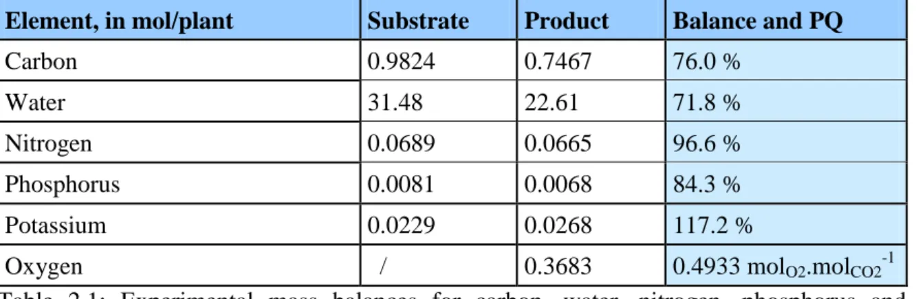
Table 2.1: Experimental mass balances for carbon, water, nitrogen, phosphorus and potassium; oxygen photosynthetic quotient. ... 63

Table 2.2: Experimental mass balances for carbon, water, nitrogen, phosphorus and potassium; oxygen photosynthetic quotient taking into account chamber leakage rate. ... 65

Table 2.3: Biomass growth behaviour depending on the considered law. ... 90

Table 2.4: List of the environmental conditions and the experimental value used in the model. ... 98

Table 2.5: List of the architectural parameters, the value and origin. ... 98

Table 2.6: List of the physical parameters, the value and origin. ... 99

Table 2.7: List of the biochemical parameters, the value and origin. ... 100

Table 2.8: Architectural module equations and parameters. ... 101

Table 2.9: Physical module equations and parameters. ... 102

Table 2.10: Biochemical module equations and parameters. ... 102

Table 2.11: Comparison of experimental and simulated data taking into account the leaks. 103 Table 2.12: List of the simplified parameters, the value and selected range of variability. ... 111

Table 3.1: Plant parameters remote sensing. ... 152

Table 3.2: Plant parameters direct contact measurements. ... 152

Table 3.3: Plant parameters destructive measurements... 154

Table 3.4: Air and canopy measurement and control devices. ... 156

Table 3.5: Nutrient solution measurement and control devices. ... 158

Table 3.6: Main requirements for a higher plant growth chamber designed for modelling implementation and validation. ... 164

(17)

Abbreviations

BM Biomass

CESRF Controlled Environment Systems Research Facility (CA) DM Dry Matter content in biomass (%)

DWC Deep Water Culture

EC Electrical Conductivity

EFM Elementary Flux Modes

ESA European Space Agency

GC Gas Chromatography

HPS High Pressure Sodium light bulb LA Total Leaf Area (m2leaf)

LAD Leaf Angle Distribution LAI Leaf Area Index (m2leaf.m-2soil)

LAS Leaf Appearance Stage

LD Leaf Density

LED Light-Emitting Diode

MAS Mathématiques Appliquées aux Systèmes (F) MELiSSA Micro-Ecological Life Support System Alternative MFA Metabolic Flux Analysis

MH Metal Halide light bulb

NDVI Normalised Difference Vegetation Index NFT Nutrient Film Technique

PID Proportional – Integral – Derivative PQ Photosynthetic Quotient

PRI Photochemical Reflectance Index

PT Physiological Time

PyGMAlion Plant Growth Models Analysis and Identification software QY Quantum yield parameter (molCO2.molphoton-1)

RD Rood Density

RH Relative Humidity (%)

RL Root Length

RUE Radiation Use Efficiency

SCK-CEN StudieCentrum voor Kernenergie – Centre d’Etude de l’Energie Nucléaire (B) SLA Specific Leaf Area (m2leaf.g-1dry biomass)

SRC Standardised Regression Coefficient

TT Thermal Time

UV UltraViolet light

VITO Vision on Technology company (B) VOC Volatile Organic Compound

VPD Vapour Pressure Deficit (Pa)

(18)

Atoms and molecules

ABA Abscisic acid

ATP Adenosine triphosphate

C Carbon

Ca Calcium

Cl Chloride

CO2 Carbon dioxide

DNA Deoxyribonucleic acid

FADH2 Flavine adenine dinucleotide (reduced form)

H Hydrogen

H+ Proton ion

HCO3- Bicarbonate ion

K Potassium

Mg Magnesium

N Nitrogen

N2 Molecular nitrogen

NADH Nicotinamide adenine dinucleotide (reduced form)

NADPH Nicotinamide adenine dinucleotide phosphate (reduced form)

NO3- Nitrate

NH4+ Ammonia

O Oxygen

O2 Dioxygen (molecular oxygen)

P Phosphorus

RNA Ribonucleic acid

RuBisCO Ribulose Bisphosphate Carboxylase-Oxygenase

(19)

Scientific parameters and variables

notations

A Sap vessel section (m2)

A Matrix of stoichiometric coefficients a Air bubble radius (m)

a Root radius (m)

a Empirical parameter for stomatal conductance calculation (dimensionless) Ac Carbon assimilation rate for carbon-limited case (mol.m-2.s-1)

Aq Carbon assimilation rate for light-limited case (mol.m-2.s-1)

aw Water activity (dimensionless)

b Soil buffer power (dimensionless)

BCmol Biomass C-molar mass (gdry biomass.molC-1)

C* Saturating concentration of CO2 dissolved in water

Ca Atmospheric CO2 concentration (mol.m-3)

Ci Internal leaf CO2 concentration (mol.m-3)

cp Atmospheric specific heat (J.kg-1.K-1)

Cs CO2 molar fraction at the leaf surface (molCO2.mol-1air)

D Gas or nutrient diffusion coefficient (m2.s-1)

D0 Empirical parameter for stomatal conductance calculation (Pa)

Dc CO2 diffusion coefficient (m².s-1)

Dens Planting density (number of plants.m-2)

DMratio Dry matter content per water content in biomass (=DM/(1-DM)) E Flux of water transpired (kg.m-2.s-1)

f Friction energy loss factor for gas movement (dimensionless) Fn Functions calculating the model’s output

G Leaf normal distribution to light ray zenith angle G Soil heat flux (W.m-2)

g Gas conductance parameter (m.s-1) g Gravity vector (m.s-2)

g0 Minimum stomatal conductance (mol.m-2.s-1)

gc CO2 conductance (m.s-1)

gs Stomatal conductance (mol.m-2.s-1)

gw Water vapour conductivity

H Plant height

I Electrical current intensity (A)

I Absorbed light flux (µmolphoton.m-2.s-1)

I0 Incident light flux (µmolphoton.m-2.s-1)

I0diff Incident diffuse light intensity (µmolphoton.m-2.s-1)

I0dir Incident direct light intensity (µmolphoton.m-2.s-1)

Ish Shaded leaves absorbed light flux (µmolphoton.m-2.s-1)

Isun Sunlit leaves absorbed light flux (µmolphoton.m-2.s-1)

J Vector of the reaction rates

J Matter exchange flux (kg.m-2.s-1 or mol.m-2.s-1) J* Root active uptake flux

J*max Maximum flux of root active uptake

Je Electron flux from photosynthetic light reactions (mol.m-2.s-1)

(20)

Jr Phloem vessel radial flux (m3.m-2.s-1)

Js Nutrient absorption flux (mol.m-2.s-1)

Jw Water absorption flux (m3.m-2.s-1)

k Light extinction coefficient

k Heat conductivity coefficient (W.m-1.K-1) k1 Ratio leaf area/fresh biomass (m²leaf.g-1)

k2 Ratio stem length/fresh biomass (mstem.g-1)

k3 Ratio sap vessel radius/fresh biomass (mvessel radius.g-1)

k4 Ratio sap vessels number/fresh biomass (number of vessels.g-1) k5 Ratio number of sap vessels/stem length (number of vessels.m-1) Ka to Kl Constants of simplification of the equations

kb Theoretical light extinction coefficient in the case of black leaves

Kc RuBisCO Michaelis constant (mol.mol-1) of carboxylation

Km Root active uptake Michaelis constant (mol.m-3)

Ko RuBisCO Michaelis constant (mol.mol-1) of oxygenation

kdir Light extinction coefficient for direct radiation

kdiff Light extinction coefficient for diffuse radiation

L Length of the conduction path (m) Lstem Stem length (m)

M Water molar mass (kg.mol-1) Ms Solute molar mass (kg.mol-1)

nT Total number of air moles in the plant growth chamber

Nvessel Sap vessels number

P Pressure (Pa)

P0 Atmospheric saturating vapour pressure (Pa) PH2O Water vapour pressure (Pa)

Ptot Total pressure

P/2e- Ratio of the production rates of ATP and reduction power of two electrons for photosynthesis (ATP/NADPH)

P/O Ratio of ATP production rate and consumption of the reduction power of two electrons for respiration (production of 1 mole of water from ½ mole O2)

Q Gas flow (mol.day-1) Q Heat flux (W.m-2)

R Vector of the rates of exchange of molecules with the external environment R Ideal gas constant (J.mol-1.K-1)

r Gas resistance to diffusion (s.m-1)

R² Coefficient of determination defining the model’s linearity ra Atmosphere resistance to water vapour diffusion (s.m-1)

re Electrical resistance (Ω)

Rleaf Total leaf surface equivalent radius (m)

Rn Energy flux of sun radiation (W.m-2)

rs Bulk canopy resistance to water vapour diffusion (s.m-1)

rx Xylem tissue resistance (Pa.m.s.kg-1 = s)

RH2O Water vapour transpiration rate (coupling state variable) (mol.s-1)

Rvessel Sap vessel radius (m)

Rd Dark respiration (µmol.m-2.s-1)

Resp Ratio CO2 release/CO2 uptake for the calculation of the respiration rate

(molrespired.molabsorbed-1)

T Temperature (K)

(21)

U Electrical tension (V)

UCO2 Carbon uptake rate (coupling state variable) (mol.s-1)

UH2O Water uptake rate (coupling state variable) (mol.s-1)

Un Set of the input conditions defining the plant environment

v Darcy’s flux of water at the root surface (m3.m-2.s-1)

V Variance

V Volume (m3)

Va Atmospheric vapour content

VH2O Water molar volume

Vi Leaf internal vapour concentration

Vmax Maximum carboxylation rate of RuBisCO (mol.m-2.s-1)

v∞ Bulk air speed (m.s-1)

Xi Model’s parameters

Y Model’s result

yCO2 CO2 molar fraction in the atmosphere

(22)

Greek Letters

α Thermal diffusion coefficient (m2 s-1)

α Empirical parameter for stomatal conductance calculation β Empirical parameter for stomatal conductance calculation Γ Photosynthetic CO2 compensation point (mol.mol-1)

γ Psychrometric constant (Pa.K-1) γ Surface tension (N.m-1)

Δ Gradient of concentration, pressure or temperature δ Boundary layer thickness (m)

δ Empirical parameter for stomatal conductance calculation δ Slope of saturation vapour pressure-temperature curve (Pa.K-1) η Air kinematic viscosity (m2.s-1)

θ Light ray zenith angle θ Soil water content

κ Permeability of the root tissues (dimensionless) Λ Root hydraulic conductance (m3.m-2.s-1.Pa-1) λ Latent heat of water evaporation (J.kg-1) µ Xylem sap dynamic viscosity (Pa.s) ρ water density (kg.m-3)

ρa Atmospheric density (kg.m-3)

ρdir Direct light reflection coefficient

ρdiff Diffuselight reflection coefficient

σ Light scattering coefficient

σ Root membrane reflection coefficient (dimensionless) Φ Light ray azimuth angle

Φ Concentration (kg.m-3 or mol.m-3) Φc Internal CO2 molar fraction (mol.mol-1)

Ψe Leaf epidermis water potential (Pa)

Ψi Internal water potential (Pa)

Фmin Minimum concentration under which the root uptake rate is null

Φo Internal oxygen molar fraction (mol.mol-1)

Ψl Leaf water potential (Pa)

Ψm Matrix pressure (Pa)

Ψo Osmotic pressure (Pa)

Ψp Hydrostatic pressure (Pa)

Ψs Nutrient solution water potential (Pa)

(23)

(24)

(25)

(26)

Foreword

The project of higher plant growth modelling for life support systems has been developed jointly for two aspects: the global model design with a specific accent on mass and energy transfers, and the simulation of the biomass production at the level of the metabolism and plant growth stoichiometry. These studies are presented in the thesis manuscript of Swathy Sasidharan L. for the aspect “Higher plant growth modelling for life support systems: leaf metabolic model for lettuce involving energy conversion and central carbon metabolism” and in the present manuscript for the aspect “Higher plant growth modelling for life support systems: global model design and simulation of mass and energy transfers at the plant level”. These documents have a common foreword defining the main aspects and requirements of the project.

Life support systems requirements

Space exploration may include long-term manned missions as well as planetary explorations, which would require life support systems designed with a high degree of closure and food regeneration capability. Micro-Ecological Life Support System Alternative (MELiSSA) project of European Space Agency (ESA) is designed in the objective of providing a planetary base for continuous life support system of a small crew (from 2 to 6), recycling 100% of air, water and producing at least 40% of food.

This system consists of six separated compartments growing micro- and macro-organisms in order to fulfil all the different recycling steps. One of these is used for growing plants: they are the last step of recycling, together with another compartment cultivating the micro-algae

Arthrospira platensis (cyanobacteria); they permit oxygen, water and food regeneration from

carbon dioxide, mineralised water and light. The final aim is to be able to control the whole recycling loop in order to fulfil human needs; in this objective efficient and robust models are necessary for each compartment. They should be able to control the environment (temperature, pH, light intensity…) in order to obtain the required behaviour for the organism. Then, the compartment could provide to the rest of the loop the required amount of output in terms of gas, liquid and solid (food). The system of control is highly constrained by two specificities: multiple levels and multiple time scales. In terms of levels, four different layers can be described (Dussap et al. 2005): level 0 is the closest to the process and contains the process measurement and basic controllers for maintaining the adequate set point for an

(27)

environmental parameter. For example, temperature or pH regulations rely on heater-cooler or acid-base pumps, with a simple proportional-integral-derivative (PID) controller. Level 1 contains the system model itself, which corresponds to the present work. It states the correct value for each environmental parameter based on the system history, prediction determination and overall loop requirements. Level 2 is not specific for one compartment, but regulates all the set points in an optimisation objective in order to respond to level 3 requirements. Level 3 is the interface with the crew, who can define future events (like crew member arrival or departure) and accurate environmental tuning. This level defines the optimised response of the loop in order to fulfil these requirements. In terms of control dynamics, they are highly different depending on the different states of the matter: gas control has to be effective within few minutes, liquid control is at an hourly step, and food control is in the day scale. Also, depending on each compartment, the biological response kinetics to environmental adjustment are different and these various time scales have to be accounted in the models. For the output control, quality and security aspects have to be included: quality in terms of chemical and microbiological content to be provided to the consumers (human crew for the overall system, but also each compartment); and security for the backup systems that should be included at each key point, for each step of the closed loop process. Another important issue is that the life support system functions with uncontrolled inputs, for example CO2 production rate from

the crew cannot be predicted accurately. Additionally, these inputs may be discontinuous (crew waste production) for a system that is designed for a continuous functioning; this means that all the system is constrained by the mass balance of the overall loop, for all the chemical elements. In a mass- and volume-limited environment in space, the buffer sizes have to be small for each of the consumable (oxygen, water, food…), which means that the life support system must have a short response-time and a highly adaptable behaviour.

The current functioning life support systems recycle only air and water; the addition of food supply is possible only by higher plant cultures and cyanobacteria. The higher plant chamber cannot function without interaction with the entire loop, because plants exchange gas and produce large amounts of water vapour; then this system must be controlled in a common way for the entire life support system. This means that the higher plant growth model must be based on the same laws and structure of the models of the other compartments; these models must therefore be studied.

(28)

Higher plant compartment requirements

Concerning the higher plant compartment, the growth environment is designed as fully controlled, the supply of CO2 being issued from the human habitat. The input flow rate

corresponds to the flow rate of minerals (CO2, N-NO3 and N-NH4) coming from the previous

compartments in charge of waste degradation. Light intensity and photoperiod, temperature, humidity, nutrient solution pH and electroconductivity are adjusted. The higher plants growth model should be designed for organizing the cultures and if possible managing environment in order to control plants behaviour. The main requirements are of three ranges. First, for a closed loop it is necessary to follow mass balance principle at each step. Then the model for higher plant compartment should take into account mass balance: metabolism has to be considered, even if a simplified way with few, global stoichiometric equations is chosen. Secondly, this model is only a part of MELiSSA loop control system: it has to be able to communicate information with the models of the other compartments. As it is also a long-term implementation system, it should be built in a structured form in order to be easy to modify, just changing specific functions or adding new parts. Finally, the system will be settled in extraterrestrial places: the environmental conditions may not be similar to Earth’s conditions, especially in terms of gravity and radiations. That is why the model must be based upon known mechanisms and validated equations. This mechanistic approach of modelling could be based upon the understanding of rate-limiting processes for plant growth: the different mechanisms that happen in the organism have a maximum rate, which depend on a few parameters. For example, maximum light interception depends on leaf properties (surface, absorption coefficient…) and incident light intensity: these parameters must be included in the model in order to obtain an accurate value of light energy available for plant growth. If all the maximum rates are calculated, like water, CO2, nutrient availability, it is

possible to know which rate limits plant growth. Following all these objectives, an extensive bibliographic research was made for finding existing models of plant growth. They can be separated in three categories as described below: global models, models of physical mechanisms and models of biochemical mechanisms.

(29)

Existing plant growth models

Global models

Global models can be separated in two main types: process-based models and functional-structural models.

Process-based models consider the environment as the main driving variable for plant growth. The calculation of soil and atmosphere variations depending on climatic conditions and plant interactions permit the calculation of biomass growth and development, in a more or less detailed view. Process-based models take into account some of the growth mechanisms like light interception or water and nutrient absorption; however plant shape is usually simplified as root and shoot, and/or edible and inedible. These models aim at modelling plant growth in an explanatory way linking environment characteristics to plant growth and development; however the developmental steps are included in an empirical way (Bouman et al. 1996, Boote et al. 1998,Gabrielle et al. 1998, Brisson et al. 2008, Priesack and Gayler 2009). Functional-structural plant models are based upon plant architecture. They consider the plant shape (structure) in a detailed way; and the internal plant mechanisms are often included in a simplified, sometimes empirical way (Fournier and Andrieu 1998 and 1999, Yan et al. 2004, Allen et al. 2005, Evers et al. 2005, Cournède et al. 2006, Bertheloot et al. 2008).

Of the existing global models of plant growth, all include an original approach of specific mechanisms: process-based models are usually well-structured for all of the mechanisms, and limiting rate calculations are done for predicting water or nutrient stress and eventually pests. Even if they often contain empirical simplifications for some processes, the approach and results are mainly based on extensive experimental knowledge from agriculture results. Also, soil and atmosphere dynamics can be included in an accurate mechanistic way, and the aim of guiding agricultural practices corresponds to the objective of the life support system control. Finally functional-structural plant models include an accurate approach of morphology even if the laws of architectural growth are not really mechanistic, and an explanatory or mechanistic approach for some of the mechanisms: some of them calculate the exact repartition of light and its absorption in the leaves; others take into account a mass-balance approach for biomass repartition in the different organs, etc. That is why, even if none of them can be adapted directly to MELiSSA modelling approach, they can all give interesting ideas for building the new model. Consequently, it is necessary to take into account models of specific mechanisms in order to select suitable ones.

(30)

Physical models

The models of plant physical mechanisms are studied separately of the global plant and the influence of specific parameters or conditions are tested in detail. The main mechanisms are light interception, gas exchange, sap conduction and root uptake. Most of them have been built on mechanistic or explanatory laws.

Light interception is generally represented using Beer-Lambert law, at the global or local scale, eventually including the reflection and refraction indices, differentiation between leaves receiving direct or diffuse light, the leaf angle, height or density (repartition in space), etc (Govaerts 1996, Asner and Wessman 1997, Chelle and Andrieu 1998, Wang and Leuning 1998).

Another mechanism is the gas exchange; it happens through the stomata, small dynamic holes in plant cuticles, and depends on stomatal aperture, wind speed in external atmosphere, leaf shape, CO2 concentration difference between atmosphere and leaf. Stomatal aperture is an

important active mechanism based upon osmotic regulations which are controlled by sensing of the influent parameters like light intensity, internal CO2 concentration, atmosphere

humidity or water availability at the root level. Gas exchange depends also on the atmosphere dynamics around the leaves, leaf shape and canopy architecture. Many different types of models exist, depending if they consider atmosphere dynamics (Boulard et al. 2002), stomatal aperture (Aalto et al. 1999, Dewar 2002, Kaiser 2009), CO2 diffusion (Leuning 1995), water

transpiration (Monteith 1981) or several of these mechanisms (Tuzet et al. 2003, Xu and Baldocchi 2003, Zavala 2004).

The matter exchange between leaf and root happens via sap conduction vessels, which are separated into two different types depending on the sap composition, origin and role: phloem sap contains water and organic solutes produced by photosynthesis in the leaves and provide the organic substrates as building blocks for biomass production in the non-photosynthetic organs: buds, roots, fruits or grains and storage organs. For the movement of water and mineral nutrients from the roots, xylem vessels are made of dead lignified cells permitting a rapid upstream flow. Sap flow rate depends on vessel radius and length, sap viscosity and production (source) and demand (sink) powers, which are expressed as water potential. Only one mechanistic model of phloem exists, based on the pressure difference between production and consumption sites (Christy and Ferrier 1973, Henton et al. 2002). Usually only the source and sink powers of the organs and a resistance-to-transfer factor are taken into account in order to model directly biomass repartition in global models (Yan et al. 2004, Allen et al.

(31)

2005). For xylem, in many cases the transport is not considered limiting compared to evaporation mechanism of transpiration, however some models consider this resistance (Tyree 1997, Cochard 2006, Da Silva et al. 2011).

Last important mechanism is the root absorption. It depends on root architecture and morphology, nutrient and water availability, active uptake mechanisms, root permeability and pumping power which is the water potential difference. Several models exist with different parameters and structures (Fiscus and Kramer 1975, Hopmans and Bristow 2002, Roose 2000).

All these mechanisms are extensively studied and most of the models have been established for more than 30 years; however some parts remain uncertain. The mechanisms which would require some more attention for including accurate and robust mechanistic laws are the stomatal processes, the sap flow (especially for phloem sap calculation, as it is difficult to measure it experimentally and it is rarely included in the models) and the root absorption. In any case, all the existing laws should be evaluated in order to verify the applicability in the case of controlled but extraterrestrial conditions.

Biochemical models

The biochemical mechanisms exist at two levels: (i) at the cell scale, metabolism, genome transcription and translation regulations, cell multiplication and differentiation, osmotic regulations take place. (ii) At the plant or organ scale, hormonal signalling, environmental sensing and active transports are the main biochemical mechanisms. However the latter are usually poorly described in terms of mathematical formulation, except for metabolism: the role of each hormone, the existence of the sensing systems and the signalling cascade, the cell multiplication and differentiation regulations especially concerning transcription and translation regulations, are not totally understood or known. The large variety of cultivars has given the opportunity to include the genetic variability into some process-based models in order to predict the response of each cultivar to the environment; however the mechanisms of resistance to a specific pest or environmental stress are not known in detail and the inclusion of cultivar genetic specificities is purely empirical (Bertin et al. 2010). In the contrary, several modelling tools are available for metabolism; all of them follow mass-balance principle using stoichiometric equations: they are the link between matter and energy exchange laws of the physical mechanisms and biomass growth and composition. For the others biochemical

(32)

mechanisms, they could be included in an explanatory way for the known mechanisms, for example as global laws of development regulation and environmental sensing.

Important approaches: Mass balance and steady state

As MELiSSA loop is designed as a continuously running closed artificial ecosystem, the mass and energy inside the loop are essential to be balanced. For the modelling of any process inside the loop, we need to consider all mass balances, either at steady state (or pseudo steady state for the gas) in batch or fed batch for the growth of higher plants. Every biochemical system maintains mass and energy balances during its growth. The matter entering into a system must, either leave the system or accumulate in the system, with or without having reaction. Then, the simplest expression for the total mass balance for the system is (Himmelblau 1967):

Input – Output + Reaction = Accumulation

The accumulation can either be positive or negative, depending on the fact that whether a compound is produced or consumed in a reaction. It should be zero at steady state. Pseudo steady state is relevant for systems observed during a long period of time. When biological systems achieve steady states (at some stages of growth), the accumulation term is considered as zero. This is generally a non growth situation, where the inputs are used for the energy production and used for the maintenance process, and in that case accumulation is zero. During growth, substrates are injected to the system (inputs) and products formed outside (outputs); accumulation occurs causing the formation of new cells.

When we take stoichiometric equations for biomass transaction in plants, we account the elements C, H, O, N and S, since others (P, Ca, Mg, K, etc.) participate only in small fractions and contribute in small quantity to the biomass. Considering plants as the biosystems, the substrates consumed are carbon dioxide, water, nutrients, light energy, etc. and the main products are biomass, transpired water and oxygen gas. Therefore, according to mass balance theory,

Substrates (inputs) → Biomass (accumulation) + (water + gases) (outputs)

In the plant system, the material balance involves the metabolic reactions and the flow of substrates: inputs and outputs, accounting the elemental balances with the surroundings. At steady state (or if assuming pseudo steady state), the concentrations of intermediates in a metabolic pathway (necessarily) remain constant, as the rates of formation is in exact balance with the rates of degradation; only the concentrations of inputs and outputs change with time.

(33)

Thus, a single rate applies to all of the reactions, when the system is in steady state (Cassimeris et al. 2011). As long as the rate of change of concentration of all intracellular metabolites is small compared to the fluxes producing or consuming metabolite, steady state approximation gives a valid approximation for the growth of the plants in the chamber and thereby modelling.

Stoichiometric metabolic model revealing plant physiology

With respect to the characteristics of the plant, plant physiology and the various mechanisms which control the growth differ. Though almost all plants have the same central carbon metabolic pathways, the reactions occur at different rates and vary from tissues to tissues, organs to organs. This may be influenced by environmental conditions which are simulated by the physical models. Therefore, for the biochemical model validation, it is necessary to verify the experimental data (input/output flux rate and mass balances) of plants grown under a predetermined/known environmental system. Furthermore, to obtain a generic plant biochemical model, a minimum of three separate metabolic models (leaves, stems and roots) should be taken into consideration which can interconnect one another on the basis of ‘carbon source’ flux transport. In this aspect, plant composition at organ level is necessary for the modelling.

A stoichiometric metabolic model refers a selected list of reactions and associated properties, assumed to be present in the system under investigation, along with the description of the environment within which the system is assumed to reside. Plant metabolic model accounts for all the major pathways like photosynthesis, respiration, energy for maintenance, and growth. The stoichiometric equations representing these metabolic pathways reveal the total impact of various constraints for plant growth predicted by the physical submodel such as, light energy availability, environmental stress, temperature, humidity, nutrient/water availability, CO2/O2 gas level, etc. All of these cellular metabolic pathways must join up in

order to attain a metabolic model, since plants can make their own constituents from a small set of precursors (CO2, water, light, mineral nutrients, etc.). The initially formed metabolites

transform and are moved by transport mechanisms, connecting the metabolism from one cell compartment to another (e.g., carbon transport from chloroplast to cytoplasm). This process takes place within the cell, from cell to cell and from organ to organ so that it connects all metabolisms, forming a large network which could integrate into the plant level. Then, the question may arise regarding the representation and analysis of the plant metabolic network.

(34)

equations of plant metabolism, which allows performing various types of metabolic network studies like metabolic flux analysis (MFA) and elementary flux mode (EFM) analysis. Both offer great opportunities for studying meaningful functional and structural properties of metabolic networks, which couple physiological perturbations and energy exchange with respect to physical limitations (e.g. light availability), thus providing the link between matter and energy exchange laws of the physical mechanisms in addition to the biomass growth and composition exploration.

Approaches to achieve the metabolic model

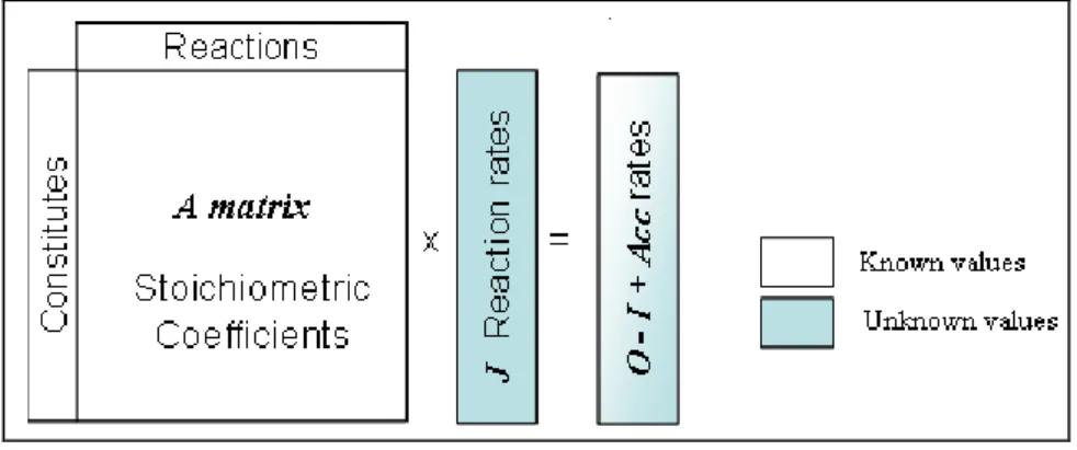
Since 1986, when Holms applied the stoichiometric approach for the growth of E. coli, several metabolic modelling techniques have been developed (Holms 1986). From the current knowledge, the most suitable stoichiometric metabolic techniques which run under steady state are elementary flux mode analysis and metabolic flux analysis. EFM analysis is specifically used to find the set of thermodynamically feasible metabolic pathways that span all the space of metabolic routes from substrates to products. On the other hand, MFA is used to calculate intracellular fluxes for the same. In order to perform these studies on a particular metabolic network, it is necessary to represent the mass balanced stoichiometric equations of that network in the form of matrices. Mathematically, the mass balance in any metabolic system can be written as,

A J = R

‘A’ is the matrix of the stoichiometric coefficients of all the reactions involved in the metabolism having the dimension of (m  n), where ‘m’ is the number of metabolites in rows and ‘n’ is the number of reactions in columns. Therefore, each column in the matrix represents a reaction. ‘J’ is a vector of the ‘n’ reaction rates.

The ‘m’ metabolic constituents are divided into two categories: the exchangeables that enter both the biotic and the abiotic phase and the non exchangeables known as intermediate metabolites. The elements of vector ‘R’ (the rates of exchange) corresponding to the intermediate metabolites must be necessarily equal to zero, as we assume steady state. The non-zero elements of R are the net rates of formation of substrates, metabolic products and biomass components which are the exchangeables.

The leaf metabolic model can be constructed using the whole set of equations corresponding to the leaf; it is necessary to collect all associated metabolism, and construct a complete metabolic network in the form of matrices as in the Figure A.

(35)

Figure A: In silico representation of the metabolic network including the mass balance description.

O = output, I = input; Acc = accumulation.

Design of a new model

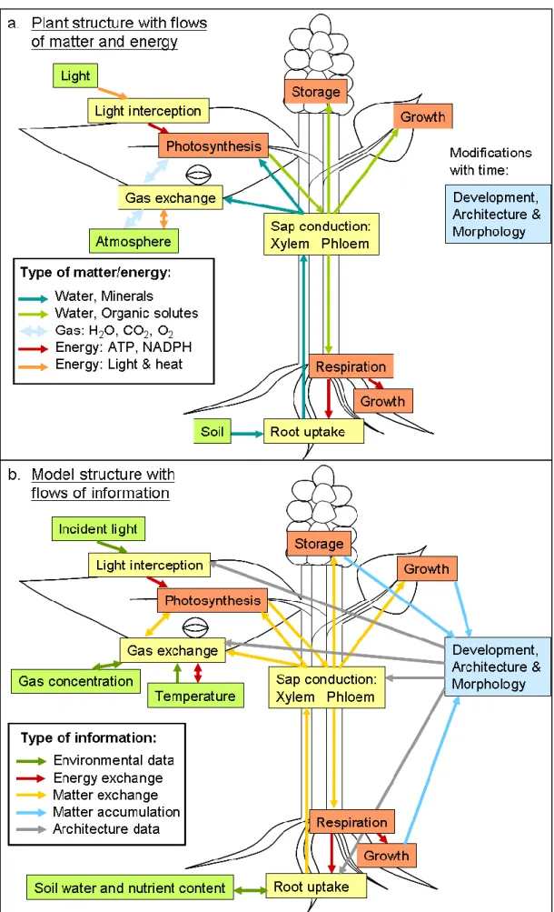
With this knowledge of plant growth modelling, it is possible to design a global model based on the physical and biochemical mechanisms described above. This corresponds to the structure of a process-based model. However, it should include a detailed description of plant architecture, as for a functional-structural model. Last requirement is to add a correct mass-balance approach with metabolic stoichiometries. This original model is schemed in Figure B: part a. represents the plant mechanisms for the flows of matter and energy, which have to be modelled. Part b. is the description of the designed model with the detail of the flows of information, separated as matter, energy and architecture information.

The blue boxes represent the plant behaviour depending on growth: development and architecture mechanisms, which cannot be described with simple mechanistic laws. The yellow boxes contain physical mechanisms submodels and the red boxes are specific for biochemical mechanisms submodels.

These submodels are developed concomitantly in order to achieve the entire plant growth model; the work associated has been split into two complementary projects. These two research objectives have been realised in permanent close cooperation. Red (biochemical) submodels are treated in the thesis of Swathy Sasidharan L. while blue and yellow (architectural and physical) submodels are described by the work of Pauline Hézard.

(36)

Figure B: Comparison of plant and aimed model structures describing the flows of matter, energy and information.

(37)

(38)

(39)

(40)

Introduction

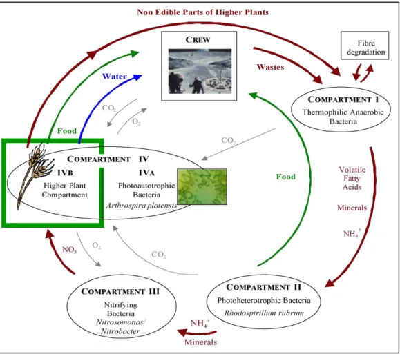
This work is included in a global project which aims at human survival in an extraterrestrial environment with a minimum supply of matter and energy: this is the definition of closed ecological life support systems. This is possible if wastes are degraded and fresh air, water and food are produced; it requires a complex community of living organisms including higher plants. Additionally, this complex community must be perfectly controlled in order to ensure the adequacy between human needs and life support system outputs. Then the importance of adaptive, mechanistic models based on mass and energy balances becomes obvious. The MELiSSA project is designed with five steps for a complete recycling loop. The first one is the first degradation step; a thermophilic anaerobic bacterial community performs the fermentation of the organic wastes (human wastes and inedible parts of the plants) into water, CO2, volatile fatty acids, ammonia and mineral salts. The second compartment is a

photoheterotrophic reactor, growing the bacteria Rhodospirillum rubrum in order to further degrade the volatile fatty acids into CO2 and produce edible biomass. The third compartment

is an aerobic fixed-bed reactor containing a co-culture of the nitrifying strains Nitrosomonas

europaea and Nitrobacter winogradskyi. They transform the ammonia into nitrite then nitrate,

which is not toxic and permits a rapid uptake by the photosynthetic organisms. The fourth step, which is the last before the human life environment, is made of two photosynthetic compartments; one contains micro-algae (the cyanobacteria Arthrospira platensis) and the other is a closed and controlled greenhouse growing edible higher plants, as described in Figure 1.

The microorganism compartment IVA is already controlled by an efficient model (Cornet et

al. 1992), but the higher plant compartment IVB was not yet modelled, and the final design

was not perfectly defined. The aim of this work is to propose the structure and components of the final model, the results of a first approach and ways for implementing and validating experimentally the future versions.

(41)

Figure 1: MELiSSA loop design highlighting the higher plant compartment IVB.

The existing models for MELiSSA loop are based on the control of microorganism growth. The main point of these models is the definition of the limiting process, using a coupled description of mass and energy balances at the molecular level (Cornet et al. 1992). It appears that structured models, taking into account together physical processes of matter and energy exchange with the environment and biochemical models of matter and energy processing inside the organism, provide efficient results. Knowing the main variables that can be used to control the growth kinetics, it is possible to maintain an adequate environment for human crew survival; the unique condition is that human needs are within the range of the microorganisms’ possible responses. This range and the growth kinetics can be predicted and extrapolated only if the model is mechanistic: this is one of the main requirements, with the simulation of mass balance and limiting process, for life support systems control.

These main requirements are applicable also in the case of higher plant cultures; however several more constraints have to be fulfilled. Microorganisms, as per the name, are small and they can be modelled at the level of the community: the individual behaviour does not influence the global community behaviour. Then, the local conditions in space and time can be summed at the global scale and the growth reactor can be considered homogeneous, if it is