TRANSONIC AXIAL COMPRESSOR USING AN INVISCID, THREE-DIMENSIONAL FINITE DIFFERENCE
by
Guido Haymann-Haber
TRANSONIC AXIAL COMPRESSOR USING AN INVISCID, THREE-DIMENSIONAL FINITE DIFFERENCE
by
Guido Haymann-Haber
GT&PDL Report No. 145 May 1979
This research was carried out in the
Gas Turbine and Plasma Dynamics Laboratory, M.I.T., supported by the NASA Lewis Research Center under Grant NGL 22-009-383.
ABSTRACT
A computational study of the flow in a Transonic Axial Compressor has been performed. This compressor has a tip Mach number of 1.2 and an
inlet hub to tip ratio of 0.5. The numerical procedure used is a fully three-dimensional, inviscid, finite difference algorithm. MacCormack's
two-step, explicit second order accurate scheme was used. A total of 30,600 mesh points were used. The results were compared to space and time resolved exit flow measurements, and to quantitative density visualization pictures. Among the most significant features resolved by the computation, was an unusual shock structure, which had earlier been observed in the experiments. The general agreement of the computation with The experiment
is good, except in regions dominated by viscous flow. Many of the effects of viscosity can be anticipated from the inviscid flow field.
ACKNOWLEDGEMENTS
This work is mainly the result of William T. Thompkins, Jr.'s ideas. He spent a great deal of time and effort on it, and without his help this
work would have never been completed.
Jack L. Kerrebrock came up with many suggestions, and his encourage-ment was of invaluable help. Alan H. Epstein deserves special thanks for
patiently spending many hours introducing me to the misterious world of computers.
My parents, Rudi and Beatriz, are those who ultimately deserve any praise, since without their moral and financial support, I would have
never come even close to starting this work.
Finally, I feel that the girls of Boston, in their zealous efforts to distract me as little as possible, were greatly responsible for the completion of this work within a finite amount of time.
This Research was supported by NASA Lewis Research Center under Grant NGL-22-009-383.
TABLE OF CONTENTS Chapter No. 2 3 4 5 APPENDIX A FIGURES REFERENCES INTRODUCTION
NUMER I CAL PROCEDURES
2.1 Differential Equations 2.2 Coordinate Transformations 2.3 Grid Structure
2.4 Finite Difference Scheme 2.5 Boundary Conditions RESULTS OF THE COMPUTATION
3.1 Convergence Criteria Solution Accuracy 3.2 Shocks
3.3 Results
3.4 Comparison with Density Measurements
COMMENTS REGARDING THE SHOCK TERMINATION PHENOMENA 4.1 Introduction
4.2 Angles Defining a Shock 4.3 Normal Shock
4.4 Oblique Shock
CONCLUDING REMARKS AND DISCUSSION ALGEBRAIC DEVELOPMENT FOR CHAPTER 4
Page No. 9 12 12 14 17 19 21 24 24 26 27 30 35 35 36 38 43 46 49 55 82
LIST OF FIGURES Figure No.
1.1 Side View of the MIT Rotor
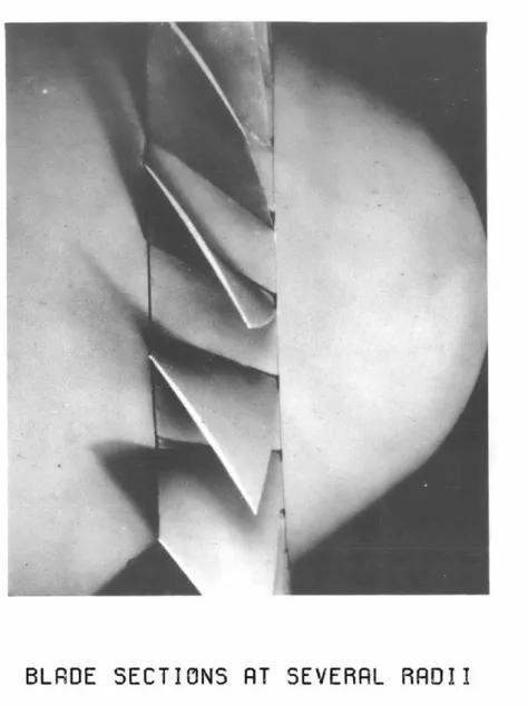
1.2 Blade Sections for Several Radii 2.1 Grid Structure in the r-z Plane 2.2 Grid Structure in the
O-z
Plane 2.3 Shock System in the 6-z Plane 3.1 Mach Number Along A Grid Line3.2 Hub to Tip Stream Surface. Pressure Surface Streamlines and Mach Number Distribution. 3.3 Hub to Tip Stream Surface. Mid-Passage.
Streamlines and Mach Number Distribution. 3.4 Hub to Tip Stream Surface. Suction Surface.
Streamlines and Mach Number Distribution. 3.5 Location of Conical Section Cuts
3.6 Isomachs at r/rt 0.65 3.7 Isomachs at r/rt 0.70 3.8 Isomachs at r/rt 0.75 3.9 Isomachs at r/rt 0.80 3.10 Isomachs at r/rt 0.85 3.11 Isomachs at r/rt 0.90 3.12 Isomachs at r/rt 0.95
3.13 Mach Number Ahead of Passage Shock or Compression Wave Vs. Radius
3.14 Flow Exit Angle in Rotating Coordinate System Vs. Radius Page No. 55 55 56 57 58 59 60 61 62 63 64 65 66 67 68 69 70 71 72
Figure No.
3.15 Location of Density Visualization Sections
3.16 Static Density Distribution at r/rt 0.70 Comparison of Computation and Experiment 3.17 Static Density Distribution at r/rt 0.80
Comparison of Computation and Experiment 3.18 Static Density Distribution at r/rt 0.83
Comparison of Computation and Experiment 3.19 Static Density Distribution at r/rt 0.88
Comparison of Computation and Experiment
3.20 Density Ratio Across Passage Shock or Compression Wave. Pressure Surface.
3.21 Density Ratio Across Passage Shock or Compression Wave. Mid-Passage.
3.22 Density Ratio Across Passage Shock or Comression Wave. Suction Surface.
3.23 Example of Criterion Used to Compute Density Ratios Across Shocks or Compressor Waves
Page No. 73 74 75 76 77 78 79 80 81
LIST OF SYMBOLS
a speed of sound
e internal thermodynamic energy h enthalpy
unit vector in direction specified by subscript n unit vector normal to solid surface
P pressure
r radial coordinate in physical domain R radial coordinate in computational domain t time
T temperature
u any velocity component (indicated by subscript) V total velocity (vector)
V total velocity (magnitude)
X axial coordinate in computational domain z axial coordinate in physical domain Z artificial viscosity term
Y specific heat ratio
e
angular coordinate in physical domain 0 angular coordinate in computational domain K artificial viscosity coefficientE intermediate coordiate in transformation p density
w rotational speed of the compressor 4, as defined on page 49
Subscripts
j
axial location of grid point k angular location of grid point L radial location of grid point n direction normal to solid surfacer radial component
s component parallel to solid surface z axial component
6 angular component
T component parallel to solid surface
o
stagnation valueSuperscripts
n indicates time step
CHAPTER I INTRODUCTION
One of today's most challenging and rewarding problems in aerodynamics is that of understanding the flow in high work transonic axial compressors.
The ever increasing requirements in pressure ratio and efficiency, while maintaining a high mass flow per unit area, make transonic or supersonic compressors a must. The cost to build and test full scale compressors of this nature is several hundred thousand dollars. Further-more, while test rigs will provide adequate information on the overall characteristics of the compressor, they will provide only partial informa-tion regarding the details of the intra-blade flow, necessary to identify the source of losses. It is for these reasons that an accurate prediction of the flow in a compressor prior to its manufacturing and testing is highly desired.
The recent advances in the field of scientific computers, have made numerical methods, like finite differences, particularly attractive for this type of application. Even relatively inexpensive minicomputers can now handle large and complex calculations at speeds, which if not adequate for iterative design, are quite acceptable for research purposes. While
in general an inviscid approximation has to be made for complex geometries in order to stay within reasonable limits of storage and computer time, ful ly viscous codes are just a step ahead with growing computer
capabilities and improved algorithms. It is the purpose of this study to compare the predictions of an inviscid, three-dimensional, finite
10'
The development of this method for application to transonic
1 2
compressors was started by Oliver and Sparis . Thompkins modified it and used it to compute the flow in the MIT Transonic Compressor. The compressor was simultaneously tested at the Gas Turbine Laboratory's
3
Compressor Blowdown Facility3. Among the measurements performed was a set of density visualization pictures, a technique developed by Epstein 4 which provides quantitative measurements of the density in the blade passages at any radial section. These pictures revealed an hitherto unobserved shock structure. While the usual two-dimensional analysis, from here on referred to as Strip Theory, predicted shocks that would gradually weaken when moving radially inwards until disapearing at the sonic line, the pictures showed shocks that were not only stronger than predicted, but that after initially decreasing in strength to virtually become a compression wave, finally ended in the form of a rather strong shock.
Thompkins was not able to clearly reproduce this behavior in the computations, and it remained unclear whether this shock structure was a purely viscous effect, or whether it was a least triggered by the inviscid flow field. Kerrebrock, Epstein, and Thompkins5 suggested a possible origin to this phenomena in the inviscid field, and this, together with a
new highly modified version of the original algorithm, constituted a motivation to recompute the flow in the MIT compressor.
In the present study, Thompkins' new algorithm was used in virtual ly the same form as reported in Reference 6. The main differences over the previous computation of the flow in the MIT rotor are the replacement of an isentropic flow assumption by a fully unsteady energy equation, a much
density. The finite difference scheme remains MacCormack's explicit two-step method, which provides second order accurate solutions.
The object of study, the MIT compressor, is described in Reference 3. Figures 1.1 and 1.2 show a view of the compressor and the shape of several blade sections. The nominal design pressure ratio is 1.6, with a measured efficiency of 91%. Tip Mach number is 1.2 and the hub to tip ratio is 0.5 at the inlet and 0.64 at the exit. The rotor has 23 blades.
Chapter 2 contains a detailed introduction to the numerical procedures. The results of the computation and comparison with experiment are
presented in Chapter 3. Chapter 4 contains a comprehensive discussion of the above mentioned shock termination phenomena. This discussion is based on the paper by Kerrebrock et al. 5, but approached from a somewhat
different direction. A general discussion of the results and conclusion is offered in Chapter 5. Appendix A contains the algebraic development that supports the discussion in Chapter 4.
NUMER I CAL PROCEDURES
2.1 Differential Equations:
The equations used to represent the flow field were the continuity equation,
-+
V
at
(PV) = 0 (2-1)the unsteady, inviscid momentum equation,
DV I
S=- VP (2-2)
and the inviscid energy equation with no heat transfer,
Dh I DP
By means of Equation (2-2), Equation (2-3) can be rewritten, Dh0 lap
where h0 is the stagnation enthalpy.
(2-3)
(2-4)
Equations (2-1), (2-2), and (2-4) can be written in weak conservation law form and expressed in matrix form in a cylindrical coordinate system as follows:
au+ + + 2
= KH
-t F -6- 5
K
(2-5)rp rpu r 2 rpur r(pur2+P) U rpu0 F rpuru rpuz rpu ruz rEt rur(Eg+P) Pu0 rpuz 0 2 p u+ rpu u+P) +
puru rpuruz pu+e
G*= Pu2+P H =rpuu K= -puu
2
Pu uz r(puz2+P) 0
u0 (Et+P) ru (E t+P) 0
2 2 2 2 2
Et = p(e + V /2) V = ur + u2 + UZ
In addition, the working fluid is assumed to be a perfect gas in thermodynamic equilibrium. The equation of state may be written
P = pe(y-l) (2-6)
It is desirable to apply the boundary conditions at a fixed spatial location, therefore a coordinate system rotating with the compressor is required. The new independent variables are:
t' = t
r= r
(2-7)
S-or
z=
z
I4
For this new set of variables Equation (2-5) becomes aU U aF aG* aH
U @
-+
lr-
+ 3-' + -K (2-8)3t
o'6-
arl
el
9z'
Dropping the prime superscripts
au+ + + K (2-9)
at
9r
90
az
whereG
=G* -ok Puru - rpu r G =pu + P - orpu6 Pu Uz - corpuz ua(Et+P) - wrEtThese equations are then non-dimensionalized by a0, T0 and p0
,
theupstream stagnation speed of sound, temperature and density on the tip casing streamline, and rt, the rotor tip radius. In the remaining sections only non-dimensionalized quantities will be referred to. In addition, y, the specific heat ratio is assumed constant.
It is important to note that even though the coordinate system is fixed to the rotor, all physical quantities, including the velocities, are those seen in the absolute coordinate system.
2.2 Coordinate Transformations:
The physical domain in shown in Fig. I.1. If the flow is assumed periodic, only the region bounded by the pressure and suction surface of two adjacent blades needs to be considered. Upstream and downstream of
the blade row, a prolongation of the blade passage subtended by an angle of 27r/B, where B is the number of blades, and limited by the hub and tip casing is considered.
The physical space is sufficiently complex to render a finite difference solution impractical in that domain. The physical space is therefore mapped into a computational domain, which is a rectangular box in which the grid lines form an evenly spaced mesh, thus allowing for easy implementation of a finite difference scheme.
The mapping functions are specified as simple analytical functions. 6
These mappings, developed by Thompkins , consist of a double set. First, one which regularizes the domain, and second, one that locally increases mesh density within the blade passage and around the leading and trailing edges.
The first set of mappings is given by: r - rh (z) R = -(2-10)
rt(z) - rh z)
r h radial location of the hub rt = radial location of the tip
6
-0
(r,z)e
(r,z) -0
(r,z)s p
where 6 and 0 describe the pressure and suction surface of the blades
p s
respectively, and their prolongations upstream and downstream of the blade row.
Inside the blade row
z - z (r)
16 Outside the blade row
(az*)
L-z e(j +afz*e) zte e -0.5 (2-13)
Z 0-Z 0 + [z-ztz0t + jz z
ZJ]
eawhere z and zte are the axial locations of the leading and trailing edges, z 0 and z t0 are constants to be chosen in a way to make the
mapping function derivatives continuous at the leading and trailing edges, and z* is given by:
z - Ze upstream of the blade row
z - z downstream of the blade row
These mappings regularize the domain, align the grid lines with the leading and trailing edges, and allow them to become z = constant lines far away from the blades.
The mesh packing function is given by
A sinh (K X) + B tg [sinh (K X)] (2-14)
where
A*
2{A* sinh (K ) + B*t ~ [sinh (K )II
X x x g x
B*
B
x 2{A* sinh (K Y + B*t ~ [sinh (K
)]}
x x x
g
xA* and B* are arbitrary constants and K is a free parameter that controls
x x F
7 Merrington
The introduction of these mappings modifies the original partial differential equations (2-9). Using the chain rule:
aU +F R +F D+ 3F X +3G 9R +G D +G 3X +3H 3R lt+3R Dr + r + aX r +9R M +0 Ng ag+X H0 + R az
+ H - + -H 3X _ K (2-15)
90 az aX az
Note that because of the particular choice of mapping functions 3R/96 and X/aO are identical ly zero. The equation may be arranged in the following way.
aU + F R aH + +R F X) aG M) H a6
TiF + - R ar + 3R Tzj + -aO -r + 7)IO+ 1 0-ilEz
(2-16)
+
=
KEquation (2-16) is the final form of the equations before the differencing is applied. The members of the Jacobian matrix of the
transform, together with the radial locations of the grid points, and the normal vectors and curvatures of the solid boundaries contain all the geometry information that is needed to solve the problem.
2.3 Grid Structure
The grid structure resulting from the application of the mappings is shown in Figs. 2.1 and 2.2. There are 100 points in the axial directior4 36 of which are within the blade passage, 18 points in the radial direction and 17 in the circumferential direction, totalling 30,600 grid points.
blade twist as one moves radially outwards, as shown in Fig. 2.2. Thus the grid lines are always approximately aligned with the relative flow direction.
Solid and periodic boundaries are placed between two grid lines allowing for the application of stable, second order accurate boundary conditions, as shall be explained later. The grid lines extend about
five blade chords upstream of the leading edge, and about three downstream of the trailing edge, in order to permit the application of far field
boundary conditions as far away from the blades as possible and thus reduce possible oscillations at the boundaries.
The grid lines in the circumferential direction are at a constant axial position, thus simplifying the application of periodicity boundary conditions. However, shocks that may appear in the flow are then usually
not aligned with the grid lines, as shown in Fig. 2.3, resulting in poorer shock resolution.
Several attempts were made to model a spinner, including one that would smoothly merge with the centerline, but these attempts were
unsuccessful. High radial velocities tended to build up at the points close to the centerline, resulting in mass flow defects of the order of
5%. Since r=0 is a singular point in a cylindrical coordinate system, the implementation of boundary conditions at the centerline poses some problems. In addition, the centerline is a stagnation streamline, and stagnation points pose stability problems. In view of the above problems, the
spinner was finally replaced by a cylindrical centerbody with a hub to tip ratio of 0.3.
2.4 Finite Difference Scheme
Equation (2-16) is solved using MacCormack's8 split operator finite difference scheme. This is a two step, explicit, second order accurate, conditionally stable scheme. The difference equation in the R direction, for instance, would be:
=n
t Fn Fn9
j,k, =U,k, - Fjk, +l - j,k, tr (2-17) jHn - HnJ+ 6t A Kn Hjkt+l j pk, P.) az +tAKj.,kt Un _6tU +U F* - F* j,k,.9 2Jk,
j,k, t R -j,k,1-lJ r (2-18) + H* - H* + St A K*k -IJk,ZJ,
k, k- I z j .9k,9where
j,
k, and t respectively identify the axial, circumferential and radial coordinate of a grid point, n indicates the time step, and *indicates an intermediate provisional time step. Also
F* = F(U*) H* = H(U*) K* = K(U*)
A = [0 1 0 0 0]
Equation (2-17) is the forward step, while (2-18) is the backward step. The forward-backward sequence was permutated on succeeding time steps, a procedure that seems to enhance accuracy. Each of the operators was run with a time step as close to the stability limit as possible. They were combined in a symmetric sequence as described in Ref. 9.
MacCormack's scheme, combined with the fully unsteady nature of the equations used, results in a solution that is time accurate in its
development.
In order to stabilize the solution along steep gradients of the flow quantities, such as across shock waves and near the leading and trailing edges, artificial viscosity terms were introduced, that add to the numer-ical damping of the scheme. The form of these terms for the R step is:
Z n+l u1n - n U n - Un
j k,A 9 r ,k, j.kt-i j,k,9+l jUk,4]
(2-19)
- un - un U n - Un
r .,k,+l rJk,Y j,k,k Uk,-l.}
j-
where K is a parameter that controls the strength of the artificial
viscosity terms. Low values of K produce sharp shocks, but result in unacceptable oscillations downstream of the shock. High values of K yield smooth solutions, but also very wide shocks and strong distortions to the
inviscid field. The proper value is somewhat problem dependent. A value of K equal to 0.4 was used.
With the addition of artificial damping, shocks appear then as regions of high gradients in velocities, pressures and densities. If a shock is aligned with the grid lines, typically 3 to 5 mesh points are required to resolve it (see Roache10 and Taylor et al. ). For the present case
however, Fig. 2.5 shows that in general shocks are at an angle to the grid lines, which increases the shock thIckness to about 5 to 9 mesh points.
2.5 Boundary Conditions:
The implementation of no-through flow boundary conditions at solid surfaces with second order accuracy is quite complex and is described in detail in Ref. 6. The basic idea consists in placing auxiliary grid points outside the flow domain in such a way that the solid surface is
located between these points and the first set of interior points. The values of the flow parameters at the auxiliary points are chosen in a way to reproduce the no-through flow boundary condition at the solid surface these values are chosen as follows:
sol id -* surface ppoint outer point u n 2 2 DOb u s+ u .T _ b i R s R T
1
subscript indicates inner pointa subscript indicates auxiliary point
b subscript indicates point on surface = -u a u = S. a I (rp) a= (rp). -2 z re I r (2-20) (2-21) (2-22) (2-23) n.
R and R are the radii of curvature in the s and T direction. The physical reasoning and assumptions underlying the use of reflection in this grid
12
system are explained by Roache .Outside the blade passage, periodicity is applied in the circumfer-ential direction. This is particularly simple for the system of offset points since there are no points on the symmetry boundary itself and thus no assumptions have to be made regarding the value of the flow quantities at those locations. Also, the fact that circumferential grid lines are at constant axial location avoids the need for interpolations.
The upstream boundary condition is applied at the first grid plane 13
by using a program developed by Berenfeld . This program uses an analyti-cal linearization of the theory of perturbations developed by Tan and
McCune 14 The program uses the flow conditions at the second axial grid plane and calculates the flow quantities at the first axial grid plane.
In order to do this, the flow upstream of the second grid plane is assumed compressible, inviscid, isentropic and steady. This flow can then be described by linearized flow equations. Far upstream boundary conditions are uniform, non-swirling flow. Three-dimensionaI perturbations proved to be very small when initially calculated. Presumably they could build up over many repeated cycles, but because of the large amount of computer time involved in calculating them at every step, they were neglected. A possible way to avoid this problem while keeping three-dimensional pertur-bations would be to update them periodically after a certain number of steps.
The downstream boundary condition, applied at the last axial plane assumes an axisymmetric radial equilibrium with the same total momentum
in the circumferential direction as that in the previous grid line. The static pressure at the hub is specified. The downstream boundary condi-tion has several inadequacies, among them that it ignores perturbacondi-tions which do not decay far downstream, and that there is certain degree of arbitrariness in the circumferential momentum averaging process. A similar procedure as for the upstream boundary was being developed by Berenfeld 3, but unfortunately it did not become operational in time to be used for this computation.
The Kutta condition is applied at the last points on the blades. At these points the usual no-through flow boundary conditions are applied, except for the pressures, which are set as though it were a periodic
boundary. In this way, the points at the trailing edge, although physi-cally only one set, are logiphysi-cally two sets of points and the pressures are identical at the "fictitious" points. No attempt is made to directly set the velocities at the trailing edge, since there are really no points on the trailing edge itself. By following the above procedure one hopes that the direction of the velocity in a plane normal to the blade axis at the point next to the pressure surface, is similar to that at the point
next to the suction surface at a given radius.
The final solution shows that for the grid points just following those on the trailing edge the above difference varies between 14* at the
hub to 4* at the tip. This difference is down to 4* or less five grid points, or about 8% chord, downstream of the trailing edge. Considering that the angle between the pressure and the suction surface tangents at the trailing edge is of the order of 35* at the hub, it seems that the Kutta condition works in an acceptable manner.
CHAPTER 3
RESULTS OF THE COMPUTATION
3.1 Convergence Criteria and Solution Accuracy
The finite difference program was run at MIT on the Gas Turbine Laboratory's PDP 11/70 computer. In its present configuration about 270 hours of running time are required for a converged solution for a new
rotor. The main limitation is disk I/0 (RK05 disk drives were used), which makes up over half of the total time.
The parameters specifying the operating point of the compressor are the upstream stagnation temperature and pressure, the rotor speed, and the downstream pressure. The mass flow is a result of the computation and is not explicitly specified anywhere. Consequently, a uniform mass flow at all axial planes is a good criterion for the convergence of the solution.
This convergence was attained to a remarkable degree, with about 1% variation of mass flow between any two axial planes in the flow domain. However, a low frequency oscillation persisted accompanied with some small mass flow variation, particularly at the downstream boundary. Also some streamline movement could be observed. Shock strength and position did not change substantially though.
Rothalpy is not expressedly conserved in the flow equations used. Therefore, a second criterion for solution accuracy is to check how well Euler's steady state turbine equation holds. At the hub, the computed total enthalpy increase across the rotor was virtual ly idential to the work corresponding to the computed induced swirl. However, they differed by as much as 10% at the tip. This number may indicate the limits of
accuracy with which total temperatures can be predicted. Some further running may better this result by getting closer to a steady state.
The averaged computed total pressure ratio across the compressor was about 1.8, as compared to the nominal design point of 1.6, at which the experiments were conducted. Attempts to reduce the pressure ratio by
decreasing the downstream pressure failed to bring about any noticeable change within a reasonable number of cycles. One cause of this problem
lies in the fact that the information is carried upstream on a wave travelling at speed uz - a, and because of the small time step allowed, a large number of cycles is required in order to transmit upstream the effect of the reduced downstream pressure.
The average computed efficiency was about 88% as compared to 91% measured in the experiments. It was particularly low at the hub. There are two possible reasons for this problem. The first is the initially low total pressure at the hub in the upstream region. This fluid when convected downstream, lowers the total pressure and thus the efficiency behind the compressor. This hypothesis was confirmed when after further running the efficiency at the hub rose sharply bringing the average efficiency up to 92%. The second source of inefficiency is the artificial viscosity. The artificial damping terms are large wherever steep flow gradients exist, regardless of whether they are compressions or expansions. Figure 3.1 shows a sample plot of the Mach number versus axial position along a grid
line. It can be seen that the Mach number gradient in the expansion preceeding the passage shock is about as steep as the gradient in the shock itself. The damping terms are therefore large in that region and entropy can increase considerably. There also are steep gradients in
the radial velocities along the hub, which cause the artificial viscosity to lower the efficiency at lower radii. Attempts to attenuate or eliminate the artificial viscosity terms upstream and downstream of the blades
resulted in instabilities, and these methods were not pursued any further. The efficiency is very sensitive to slight changes in the total pressure or temperature ratios and may have a relatively large error.
In any event, the computation was stopped once good mass convergence had been achieved since most of the interesting features of the flow had already appeared.
3.2 Shocks
As mentioned earlier, shocks are resolved as regions of steep gradients of the flow quantities smeared over 5 to 9 mesh points in this problem. This makes it difficult to distinguish between shocks and compression
waves, and the boundary between them is not clear cut.
Another characteristic of MacCormack's scheme is that shocks are preceded by an overshoot and followed by an undershoot of the Mach number (see Roache10 and Taylor et al. ). This effect is usually a good indi-cation of the starting and termination points of a shock. For the flow
in the compressor however, the shock is preceded by a very strong expansion and correspondingly fast increase in the Mach number, and followed by a continuing compression as the passage extends towards the trailing edge.
In most cases these compressions and expansions are strong enough to completely blur out the expected overshoots, resulting in an uncertainty
in shock strength and position. The problem is clearly seen in Fig. 3.1. The criteria adopted here is to consider the shock to lie in the steepest part of the compression curve.
3.3 Results
With the above considerations in mind, we may look at the resulting flow in the compressor.
Figures 3.2, 3.3 and 3.4 show the Mach number distribution for three different hub to tip streamsurfaces. The streamlines on these surfaces are also shown. On the streamsurface closest to the pressure surface the
flow is al I subsonic. Since shocks spread over a finite number of grid points, and since there is no trace of steep Mach number gradients on the blade, the shock must be detached. On the other two surfaces the shock can be recognized as a region of steep Mach number gradient, and the difficulty of determining where the shock weakens into a compression wave becomes apparent.
The striking feature on these surfaces is that the flow is supersonic virtual ly all the way down to the hub, whereas strip theory predicts a sonic line at about 80% of the tip radius. A strong upward curving of the streamlines occurs within the shock, which is expected since the flow meets relative to the shock at an angle of less than 900. At higher radii, the streamlines curve downwards immediately fol lowing the shock.
On the suction surface, the lower streamline almost meets the hub towards the end of the passage, while on the pressure surface it stays at
an about constant distance from it in spite of the area reduction. This could be an indication of trailing vorticity due to spanwise variation of the loading on the blade.
Figures 3.6 through 3.12 show isomachs for a series of conical sections around the compressor, chosen so as to approximately follow the
is shown in Figure 3.5.
The source of the high Mach numbers near the hub section becomes apparent as a strong expansion around the suction surface behind the
leading edge. At a leading edge radius of 0.65 the supersonic region already spans most of the passage originating a compression wave behind the supersonic bubble thus formed. At a radius ratio of 0.70 a double compression wave develops; one ahead of the passage, and another behind
the passage.
At a radius of 0.75 it is already difficult to tel I whether there is a compression wave or a shock in the passage, but at 0.80 the isomachs are close enough to warrant assuming a shock exists. The shock is clearly detached. It is difficult to judge however, whether the side extending ahead of the passage forms a bow shock or a compression wave, mainly because the mesh spacing gets quite coarse when moving away from the leading edge. At higher radii it turns out that the distance between the isomachs is equal or less than the spacing between the grid points. Therefore, even though the isomachs may appear quite separated a bow shock may actually exist.
The region just ahead of the leading edge is in general subsonic, as would be expected for a detached shock. However, the suction surface behind the leading edge is supersonic, which is particularly clear at higher radii. It is unlikely that a real flow would become supersonic
immediately behind the leading edge, and this phenomena is possible due to insufficient number of grid points and inadequate grid structure around the leading edge, in order to handle the high angle of attack of the
care.
A look at the Mach number ahead of the passage shock reveals that it increases steadily up to a radius of about 0.80. At 0.85 it is virtually the same for most of the passage, whi le the isomachs seem just as close as they were on the lower radius. It is not until a radius of 0.95 that the Mach number continues its upward trend and the isomachs close in further.
Figure 3.13 shows a plot of the Mach number ahead of the passage shock or compression wave. On the pressure surface the Mach number
increases monotonically except for a mild flattening at the radius ratio of about 0.86. However, moving towards the suction surface a definite peak
in the Mach number appears at a radius of about 0.80 midway between the blades and at about 0.77 on the suction side. This is the first evidence of the shock structure mentioned in the Introduction.
It is interesting to note that a rather strong compression takes place on the suction surface towards the trai ling edge, in order to meet the Kutta condition. In a real fluid the strong adverse pressure gradient associated with this compression would considerably thicken the boundary
layer on the blade, and perhaps even separate it. The thick boundary layer would reduce flow turning and drop the total pressure ratio. This could be a contributing factor to the discrepancy between the pressure ratio predicted by the computation and the measured one.
Finally, the relative coordinate system flow angles behind the trailing edge are compared with the experimental data reported in Ref. 6. These are plotted in Fig. 3.14. The computed angles are lower by 5* to
metal angle of the trailing edge. The higher angle in the experiments would be consistent with a thick or separated boundary layer on the suction surface of the blade.
3.4 Comparison with Density Measurements
Figures. 3.15 through 3.19 show comparisons between the fluorescent density measurements performed by Epstein,4 and numerical results at several radii. The pictures are taken on a plane sheet of light as it shines
through the passage. Consequently, the radial location of each point varies as one moves from blade to blade. The numerical results are shown on a cone that approximates that plane. The discrepancies in the radii are of a few percent and are not critical to the more or less qualitative discussion to follow. This discrepancy is also the reason that the blades appear with different stagger angles for the computation and the pictures.
When comparing the results it has to be kept in mind that the exper-. imental results showed some non-periodicity, particularly in the magnitudes of the density, but also in the precise shapes of the boundaries of the
different density levels. These can change noticeably and are not to be taken as final. The trend is constant though.
Regarding the numerical solution, the shocks obviously appear smeared over greater regions than the sharp density jumps seen in the pictures.
Because of this, compressions immediately following the shocks may appear to form part of the shock itself, and in general compression waves and shocks may not look all that different. In the pictures, the densities were
refer-red to the undisturbed upstream values, which poses some problems in scaling the computed values, since sometimes there is no clear uniform upstream
At a radius of 0.70 there are several similarities between the exper-imental and computed results. Among them, a low density bubble behind the leading edge, a higher density region ahead of it, and a tendency to keep the density lower closer to the suction surface. The major differences are that the computation predicts a faster compression rate when moving towards the rear of the passage, that the low density bubble is smaller for the
experiments, and that closer to the suction surface the flow is quite differ-ent. The general density levels are similar in magnitude.
At a radius of 0.80 there is an uncertainty in the value of the
upstream density, since there is no uniform flow upstream, and consequently the computations may not be scaled correctly. This may be the reason that they predict a lower value for the density of the bubble compared to the experiments. The most important difference is that the picture shows a
shock that hits the suction surface considerably further back than predicted by the computations. The shocks are detached in both cases and the bow shocks are of similar strength, but do not extend as far into the next passage in the computations. The density increase trend behind the
passage shock is similar for both cases, except for the very high density region that appears on the pictures.
At a radius of 0.83 the density pattern midway between the blades is quite similar for the computation and the experiment, except for a faster expansion ahead of the low density bubble shown by the numerical results. Again, the size of the low density bubble is greater in the computations than in the pictures.
At a leading edge radius of 0.88, the experimental results show a lambda shock at the suction surface, signaling a strong boundary
layer-shock interaction, which can obviously not be reproduced by the Inviscid computations. The computed shock is much stronger there, and its position is now also closer to that shown in the pictures. The computed bow shock strength close to the suction surface seems greater than for the exper-imental result, mainly because of the large low density bubble extending into the next passage. The computed bow shock does not extend as far out though. Again, considering the region unaffected by the lambda shock, and not too close to the pressure surface, the density increase trend is similar for both cases.
In conclusion, the computed solution compares reasonably well with the density measurements as long as sections far enough from either blade are considered. The important differences are in the shock position and
in the size of the low density bubble. Bow shocks are in general not predicted very well either in extent or strength. The flows close to the blades can differ considerably.
In Figs. 3.20 through 3.22 there is a comparison between the density ratios across the passage shock or compression wave as predicted by the computations, and as shown by the pictures. The density ratios across compression waves are difficult to determine for the experimental results since there is no clear criteria to determine the starting and termination point of the wave from the resolution available from the pictures. These points were a little clearer in the computations. Because of this, the measured values may have some vertical shift. In the case of shocks, the numerical results tend to include into them compressions that may follow.
In order to avoid guessing shock termination points, the density ratio across the shocks in the pictures is calculated including any compressions
immediately following them. An example of how this criterion is applied is shown in Fig. 3.23.
The results are quite similar for the mid-passage region, except for the drop in shock strength, which is apparently not as large in the
computations. Some of this difference may be due to improper estimation of compression wave strength and to the fact that between a radius ratio of 0.80 and 0.90 there are only four grid points, which limits the
accuracy with which the strength variations can be resolved. The results are farther off for both the pressure and suction surface as would have been expected from the comparison of the pictures. It has to be kept in mind that experimental data close to the blade surfaces is scarce and
that therefore there are not many points in the curves of Figs. 3.20 and 3.22. The most notable feature is that even though the magnitudes of the peaks are not the same for experiment and computation, they occur at the same radial position in all three cases.
When computed density ratios are compared to those corresponding to a normal shock with the same approaching Mach number, the former turn out to be lower in general. This means that the shocks are oblique, and since the Mach number is subsonic behind them, they are strong oblique shocks. This may be somewhat surprising when considering that weak oblique shocks
seem to be the norm in external aerodyanmics. Shapiro15 suggests however that high back pressures in channel flow, as is the case in high work compressors, may generate strong oblique shocks. Since the flow is sub-sonic behind the shock, the shock has to be normal to solid boundaries, which can be verified in Figs. 3.3 and 3.4 where the shock becomes normal to the flow towards the tip. The shock angles corresponding to the
computed density ratios and Mach numbers vary between 75' and 90*, which is more or less what the above figures seem to show.
CHAPTER 4
COMMENTS REGARDING THE SHOCK TERMINATION PHENOMENA
4.1 Introduction
Perhaps the most significant result of this computation is the
confirmation that the unusual shock structure revealed by the fluorescent 5 density pictures has an inviscid origin, as suggested by Kerrebrock et al.
In that paper it is shown that if the usual strip theory assumptions are made, including that of a constant inlet axial Mach number, a discontinuity appears in the radial momentum equation at the point where the shock
terminates. Such a discontinuity cannot exist since it would attribute very different radial velocities to two points that are just one above the other.
The inviscid solution indicates that the Mach number component responsible for the drop in total Mach number ahead of the shock, is the axial component. Part of Kerrebrock's analysis is then reconstructed by
relaxing the requirement of constant inlet axial Mach number, and
requiring that the radial momentum equation be continuous. The required total realtive Mach number variation is then found.
4.2 Angles Defining a Shock
r is the angle that the relative velocity vector forms with the tangent to the projection of the shock on a plane defined by V and the r axis.
is the angle that the relative velocity vector, V, forms with the tangent to the projection of the shock on a plane defined by V and the 0 axis.
Let us look at the projection of a shock on a vertical stream-surface between two adjacent blades.
shock streamline just above shock termination blade streamline
just
below shock terminationIt can be seen that streamline splitting will occur at shock termination if the intersection of the shock surface with the vertical
stream surface is not normal to the incoming flow. If the shock is assumed to terminate at the same radius for all theta locations, there can be no fluid to fill in the gap left between the streamlines.
Consequently, the above situation is not possible and the projection of the shock on that streamsurface and the incoming velocity have to be normal to each other at the termination point as sketched below.
In the remaining part of this Chapter, the blades will be idealized as flat plates with no camber. Therefore all the work in the compressor
is done by the deceleration provided by the shock alone. Furthermore, the blades will be assumed to be very close together, so that the flow is virtually axisymmetric. An alternative way to view this, is to consider the compressor to be replaced by a special type of actuator disk composed of a shock system rotating with speed w.
Upstream of the "compressor" zero swirl and uniform total temperature and pressure are assumed. The subscript I will be used to refer to the flow just ahead of the shock, whereas 2 will denote the flow just behind
it. Prime superscripts denote quantities referred to the rotating coor-dinate system.
The central equation used is the radial momentum equation, which in cylindrical coordinates can be written
2
Du u d
r =0 IdP (4-I)
Dt -r p dr
All variables referred to are nondimensionalized as described in Section 2.1. Intermediate algebraic steps in the analysis to follow are described
in Appendix A.
4.3 Normal Shock
Let us assume that the shock is normal to the relative incoming flow at any point, that is 1r =1 = 90*. For this case it is shown in the Appendix that equation (4-1) can be written
Dur2 2
r
2 PI d P 2P1 y 2I dDt = r -7 - I 2 -_ d 2- P dr (4-2)
where
)I
+ Y-- M,2(I = y-+ M2= 2 2 1 1
(1 + Y 21Wr)2)
and VI and V' are the relative velocities ahead and behind the shock, as
1 2
shown in the sketch below, which is a projection of the shock on a surface defined by a streamline and the 6 axis.
blade
shock
(A)WV
In the region above shock termination, normal shock relations are used and Equation (4-2) can be expressed
[Y-I)M1 2 + 2][1 + yl (r) 2][3 + y - 2M 3 dM_
[(y-l)M1 2 M12
[I 2 dr shocked
2 1 regivon
= o2r 4 + 4(y-l) M,2 - (4 + 4y - (y-) 2) M,4 - 2(y2-1) MI6
Du
- y+I )2 [1 +%Y1 M12] M14 {Dr shocked
2 1 + shocked(
Below the shock all ratios are unity and also d(P2 P )/dr E 0.
Dur2 [I + Y (r) dM' 2r
- 2
2MI I(o r(4-4)
Dt below [I + iM'2 ] dr below [I + M 2
shock 2 1 shock 2 1
Assuming now that at the shock termination point the flow is axial in the absolute coordinate system, it is clear that Dur /Dt has to be continuous at that point, since otherwise streamline splitting will occur. There is no loss of generality by the above simplification, since if this
is not true Euler's equation can be expressed in a coordinate system aligned with the flow. Therefore
Du Du
r 2 r2
ust
[
Dt . u(4-5)D-just - -just
below shock above shock
The Mach number ahead of the shock has to be continuous since a slip boundary can not exist there, but dMI/dr, its variation with r, need not be continuous. Replacing (4-4) into (4-3) yields
[I + Y-(r)2 2] dM M2 [Y-1) M,2 + 2][3 + y - 2M 2
I
[I + Yi1 My 2 1 M{1 dr above 2 1 shock + (y+I)2M,
2 - (4-6) below" shock=2r [4 + 4(y-)M 2 - 2(2y+[-y2)MI4 - 2(y2 )M6
The right hand side of (4-6) is negative for M' greater than one (for the usual values of y, the specific heat ratio), and zero for MI = 1. Let us
consider each case separately.
If the shock starts at the sonic line, the right hand side of (4-6) vanishes and the equation is reduced to
dM' fdM?
dr I dr (4-7)
6 above below
shock shock
Three cases can exist:
1. dM?/dr greater than zero below the shock.
This implies that dM1/dr is less than zero above the shock. Since the shock is at the sonic line, the Mach number would have to be subsonic on both sides of the shock, and thus no shock could exist. This
possiblity is unphysical.
2. dM1/dr equal to zero below the shock.
In this case dM'/dr is also zero above the shock (and thus continuous). Taking the derivative of Eq. (4-6) it can be shown that then d2M'/dr2 is also zero at termination. Consequently an inflection point occurs for this case.
3. dM'/dr is less than zero below the shock.
dM1/dr is then greater than zero above the shock, and thus the Mach number has a minimum at shock termination, while the flow is supersonic on both sides. If the hub is not curved downwards very strongly, Du r/Dt
is greater or equal to zero in its vicinity. It can then be inferred from Eq. (4-4) that dM1/dr has to be greater than zero at the hub. Consequently M? would have to have a supersonic maximum in the unshocked region. This situation may seem somewhat unlikely, but in any event, if possible it would require the existance of a peak in the Mach number.
The next interesting case is what happens if the shock does not start at the sonic line, but at a higher Mach number. In this case the right
hand side of (4-6) is negative. All other terms on the left hand side 2
are positive, except the polinomia (3 + y - 2M1 ) that multiplies dM1/dr above the shock. For y = 1.4, this term is negative only if M is greater than 1.48. Since it is unlikely that the flow has not shocked at that Mach number, it is safe to assume that all terms on the left hand side of
(4-6) are positive. Two cases arise:
I. dM1/dr is greater than zero below the shock.
Then dM'/dr is less than zero above the shock, which is now possible since the flow is supersonic below shock termination. A maximum appears at the shock termination point.
2. dM?/dr is less than zero below the shock.
dM'/dr could be greater or less than zero above the shock depending on the value of the different parameters entering the equation. Using the same argument as for case 3 above, there would have to be a maximum for the Mach number in the unshocked region, assuming the present case is feasible.
From the study of all possible cases, it is clear that at least for normal shocks, there has to be either an inflection point or a maximum
in the Mach number versus radius curve. Whether a maximum would be followed by a minimum is not clear. For a tip of constant radius, as is the case for the MIT rotor, Du r/Dt has to be zero in that region. Equation (4-3)
dMf [(y-l) M 2 + 2][1 +
Y-1
(r)2][3 + y - 2M 2] M1 31 2 I 1 drshocked
region
= c2r [4 + 4(y-l) M 2 - (4 + 4y-(y-l)2)MI 4- 2(y 2-l) M 6] (4-8)
The right hand side is negative, and thus dM1/dr will only be greater than zero if (3 + y - 2M 2) is negative, which is only true if M is greater than 1.48 (for y = 1.4). This is fairly high Mach number and unless it
is reached there is no guarantee that the Mach number has to start
increasing again after the initial drop. Curiously enough though, in the MIT compressor, where the shock is normal at the tip, the Mach number there
is just a shade above 1.48, which would allow for a minimum.
4.4 Oblique Shock
In order to assess the effect of a slight inclination of the shock on the behavior pointed out for normal shocks, the requirement that r be 90* will be relaxed. However, in order to keep the algebra within manageable
proportions
%
will still be assumed constant and normal. This means that in a blade to blade projection the shock still looks normal, but on a hub to tip projection the shock can be angled with respect to the incoming flow. This simplification is consistent with the results of the computa-tion, which shows that the shock is almost normal in a blade to blade projection, while the angle with the incoming flow in a hub to tip projec-tion may be as low as 75*.Following the development of the Appendix, the momentum equation can then be written
[-1) M, + 2][l +Y-' (or)2
F4
sin2 Or - + y - 2M dM+ M'I I dr shocked
ry 1 region
V, 2
2 2 n cs(+d 2 [1 - M 2] 2
V' sin (r + d Cos 6 -
J
(y+l) + 1- (Y-l) M 2+ 22 M
(Y-1
n n
-4 M + 21[l [I- ( r) 2 sin r Cos ar
rDu
- (Y+I) 2 + M2
]M 2 2 (4-9)
2 1 1n shocked region
where 6 is the angle of the incoming flow with the z axis and 6d and Vn
n are respectively the deviation and normal velocity component behind the shock, both of which can be obtained from oblique shock relations. M'
n
is the normal component of the incoming Mach number, that is M' sin r Note that if 1r = 90* the above equation reduces to (4-3) regardless of the value of da r/dr. Since it has been shown that ar is 90 at shock termination, then the previous discussion is also valid for an oblique shock if the flow is approximately axial at the termination point (6 = 0) and is 90*. Therefore, the Mach number has to peak or at least have an
inflection point even if the shock is oblique. If numbers are replaced into Equation (4-9), it is found that the values of the different terms
do not change substantially from those for a normal shock if Or is not greater than about 75*. The only major difference is the addition of the d r/dr term.
The terms on the right hand side of (4-3), for normal shocks, or (4-9) for oblique shocks, are in general negative, while the terms
multiplying dN/dr on the left hand side are positive except for very high Mach numbers. It can be concluded then, that a strong downward curvature of the streamlines (very negative Du r/Dt) is required in order to keep dM1/dr positive, and this is clearly observed in Figs. 3.3 and 3.4.
In conclusion, while this analysis cannot predict the exact shock structure in the compressor, it does support the results that have been both measured and computed. The radial momentum equation, plus the continuity equation and the assumption of axisymmetric flow should prove to be sufficient to determine the shock structure if normal shocks are assumed, but the complexity of this problem puts it beyond the scope of this paper.
CHAPTER 5
CONCLUDING REMARKS AND DISCUSSION
The main objective of this investigation was to verify how well an inviscid three-dimensional finite difference computation can predict the flow in a transonic compressor. The first conculsion is that the most important qualitative features revealed by the experiments are also
predicted by the numerical computation. These include the unusually strong shocks, their detached nature, and the non-monotonical increase in shock strength when moving radially outwards.
Quantitative agreement is relatively good in regions not obviously dominated by viscous effects. The notable exceptions are passage shock position and bow shock position and strength. The latter can be attributed to insufficient grid resolution far ahead of the leading edge. The more forward position of the passage shock in the computations is possibly due to the higher back pressure associated with the higher total pressure ratio obtained in the computations.
Viscous effects are obviously quite important in the vicinity of the blades, and can sometimes influence the whole flow, as is the case for the
lambda shock. Judging from the density ratios across the shock shown in Figs. 3.20 through 3.22, viscous effects may be a major factor in contri-buting to the lower total pressure ratio measured in the experiment. A thick boundary layer on the suction surface could also be inferred from the high adverse pressure gradients on the trailing edge that had been pointed out earlier.
There are a few comments regarding the finite difference scheme. One of the most annoying problems was the slow rate at which the solution
responded to a change in boundary conditions. As commented earlier, one root of the problem lies in the small time step allowed because of high mesh density. It might be interesting to device a method that would allow to switch quickly between meshes of different densities in order to speed up the transmission of information on a coarse mesh, and refine the solu-tion on a fine mesh, each time a change is introduced. The downstream boundary conditions were apparently at fault as well, and it may be worthwhile to try to apply the downstream pressure at a point closer to the blades, or else specify the far upstream Mach number. Perhaps a
better solution would be to switch to an implicit algorithm with no time step stability limitation.
As reported, an oscillation at the upstream and downstream boundaries persisted. Better boundary conditions may avoid this problem and would also perhaps allow boundaries to be placed closer to the blades, thus saving storage and speeding up the transmission of information.
Artificial viscosity terms do present a serious problem far away from shocks, since they inevitably take out usable energy from the flow. These terms probably carry the main responsibility for the low computed efficiency. Attempts to eliminate them far away from steep gradients, and
in subsonic regions, should be continued.
Final ly, although the grid structure represents an enormous improve-ment over previous attempts, it does not produce good solutions in the viscinity of the leading edges. Also, the problem of modelling a spinner
is still unsolved.
In conclusion, the present finite difference program seems to predict with reasonable accuracy the inviscid flow field in the compressor, but
in order to obtain predictions that can be used in lieu of experimental results, viscous effects will have to be accounted for. This could be accomplished by either using fully viscous codes, or more modestly, by having independent programs predict the boundary layers from the inviscid solution, model the wakes, and iterate.
APPENDIX A
ALGEBRAIC DEVELOPMENT FOR CHAPTER 4
In this Appendix the algebraic steps leading to the equations in Chapter 4 are developed in detail.
A.1 Radial Momentum Equation for a Normal Shock
The ideal gas equation for the flow behind the shock can be written in non-dimensional form as
T
P2 P ( + 1-1 M2 )
~2
2T 22 I (A. 1-1)where a parameter
4
can be defined as2 1 CA. l-21 M = M,2 _ (&r)2 (1 +
i-
M2) 1 12 1 (A. 1-3) M2 = M,2 2 + (or)2 2 replacing into (A.1-2) yields[I +xy- M,2]
[I + Y1(r) 2 2
Behind the shock the radial momentum equation (4-1) can be
(A. 1-4)
(A. 1-5) Since
then
Dur2
_
(VI sin a2- 2 T2 _ dP2Dt r TI YP2 dr
which can be accomplished by replacing p2 by the expression (A.l-1) and u2 by VI sin a - wr, as explained in the sketch below.
n(A-)
Equation (A.1-6) can be rewritten
Du IY
*r2 2 V sin x
2_ 2 2 2
Dt = r r
where constant upstream stagnation -2
a
T P 0 d(P2 /P0T2 0 dr
T P2 # dr
pressure P0 has been assumed.
P, = PO g-I andar = VI sin~, (A.l-7) can be rewritten
Du Dt V sin a2) w2 r
LI
sin a -2 P1g-
1 d T I 2For a normal shock a2 = a * Also (T2 /TI MDI/P2 = pI/p2 , and working the derivative with respect to r in Equation (4.2) is finally obtained.
(A. 1-7)
Since