HAL Id: hal-01367455
https://hal.inria.fr/hal-01367455
Submitted on 16 Sep 2016
HAL is a multi-disciplinary open access
archive for the deposit and dissemination of
sci-entific research documents, whether they are
pub-lished or not. The documents may come from
teaching and research institutions in France or
abroad, or from public or private research centers.
L’archive ouverte pluridisciplinaire HAL, est
destinée au dépôt et à la diffusion de documents
scientifiques de niveau recherche, publiés ou non,
émanant des établissements d’enseignement et de
recherche français ou étrangers, des laboratoires
publics ou privés.
Heterogeneous Face Recognition with CNNs
Shreyas Saxena, Jakob Verbeek
To cite this version:
Shreyas Saxena, Jakob Verbeek. Heterogeneous Face Recognition with CNNs. ECCV TASK-CV
2016 Workshops, Oct 2016, Amsterdam, Netherlands. pp.483-491, �10.1007/978-3-319-49409-8_40�.
�hal-01367455�
Shreyas Saxena Jakob Verbeek
INRIA Grenoble, Laboratoire Jean Kuntzmann {firstname.lastname}@inria.fr
Abstract. Heterogeneous face recognition aims to recognize faces across dif-ferent sensor modalities. Typically, gallery images are normal visible spectrum images, and probe images are infrared images or sketches. Recently significant improvements in visible spectrum face recognition have been obtained by CNNs learned from very large training datasets. In this paper, we are interested in the question to what extent the features from a CNN pre-trained on visible spectrum face images can be used to perform heterogeneous face recognition. We explore different metric learning strategies to reduce the discrepancies between the dif-ferent modalities. Experimental results show that we can use CNNs trained on visible spectrum images to obtain results that are on par or improve over the state-of-the-art for heterogeneous recognition with near-infrared images and sketches. Keywords: domain adaptation, face recognition
1
Introduction
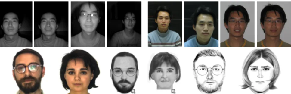
Heterogeneous face recognition aims to recognize faces across different modalities. In most cases gallery of known individuals consists of normal visible spectrum images. Probe images may be forensic or composite sketches, which are useful in the absence of photos in a forensic context [8, 14]. In comparison to the visible spectrum (VIS) images, near-infrared (NIR) and shortwave-infrared images are less sensitive to illumi-nation variation. Midwave-infrared and longwave-infrared (LWIR), also referred to as “thermal infrared”, is suitable for non-intrusive and covert low-light and nighttime ac-quisition for surveillance [9]. Differences between the gallery and probe modality, make heterogeneous face recognition more challenging than traditional face recognition, see Figure 1 for an examples of VIS and NIR images, as well as sketches.
Visible spectrum face recognition has been extensively studied, and recently much progress has been made using deep convolutional neural networks (CNN) [18, 21, 23, 25]. In part, this progress is due to much larger training datasets. For example, Schroff et al . [21] report an error of 0.37% on Labeled Faces in the Wild (LFW) dataset [5], using a CNN trained on a proprietary dataset of 200 million face images. Earlier state-of-the-art work [22] used only 10 thousand train images, yielding an error in the order of 7%.
Large visible spectrum datasets can be constructed from internet resources, such as e.g. IMDb [25], or social media websites. This is, however, not possible for IR images or sketches. For the same reason, it is even harder to establish large cross-modal datasets where we have individuals with images in both modalities. The question we address in this paper is how we can leverage the success of CNN models for visible spectrum
2 Shreyas Saxena and Jakob Verbeek
face recognition to improve heterogeneous face recognition. We evaluate a number of strategies to use deep CNNs learned from large visible spectrum datasets to solve het-erogeneous face recognition tasks. We obtain results that are on par or better than the state of the art for both VIS-NIR and VIS-sketch heterogeneous face recognition.
Fig. 1. Top: Example images of an individual in the CASIA NIR-VIS dataset (NIR left, VIS right). Bottom: Examples from e-PRIP: (left to right) photo, FACES sketch, and IdentiKit sketch.
2
Related work
Most heterogeneous face recognition work falls in one of two families discussed below.
Reconstruction based methods. These methods, see e.g. [20, 7], learn a mapping
from one modality (typically that of the probe) to the other. Once this mapping has been performed, standard homogeneous face recognition approaches can be applied. Sarfraz and Stiefelhagen [20] learn a deep fully-connected neural network to regress densely sampled local SIFT descriptors in the VIS domain from corresponding descrip-tors in the LWIR domain. Once the local descripdescrip-tors in a probe image are mapped to the gallery domain, face descriptors are matched using the cosine similarity. Juefei-Xu et al . [7] learn a dictionary for both VIS and NIR domains while forcing the same sparse coefficients for corresponding VIS and NIR images, so that the coefficients of the NIR image can be used to reconstruct the VIS image and vice-versa. The advantage of reconstruction-based methods is that allow re-use of existing VIS face recognition systems. On the other hand, the problem of cross-modality reconstruction may prove a harder problem than cross-modality face recognition in itself.
Common subspace methods. These methods learn a mapping from both the probe and the gallery modality to a common subspace, where matching and retrieval among images across the domains can be performed. Mignon and Jurie [14] adapt the met-ric learning objective function of PCCA [15] to only take into account cross-domain pairs. We explore similar metric learning approaches, but explicitly investigate the rela-tive importance of using intra and inter domain pairs, and separate projection matrices. Crowley et al . [2] use a triplet-loss similar to LMNN [24] to learn projections to map photos and paintings to a common subspace. Using CNN face descriptors [18] they obtain better performance, but do not observe improvements by subspace learning. We also use of CNN features, but instead of simply using the penultimate network layer, we also investigate the effectiveness of different layers and find these to be more effective.
Layer C11 C12 P1 C21 C22 P2 C31 C32 P3 C41 C42 P4 C51 C52 P5 S Filters 32 64 64 64 128 128 96 192 192 128 256 256 160 320 320 10,575
Fig. 2. CNN architecture: convolutions (C) use 3 × 3 filters and stride 1, max-pooling (P) act on 2 × 2 regions and use stride 2. The final soft-max classification layer is denoted as S.
Domain adaptation. Heterogeneous face recognition is also related to domain adap-tation, we refer the reader to [19] for a general review thereof. We do highlight the un-supervised domain adaptation approach of Fernando et al . [3], which aligns PCA bases of both domains. Despite its simplicity, this approach was shown to be a state-of-the-art domain adaptation method. We use it as a baseline in our experiments.
3
Cross-modal recognition approach
We describe our CNN model and how we use metric learning to align modalities. Learning a deep CNN model. We use the CASIA Webface dataset [25] which con-tains 500K images of 10,575 individuals collected from IMDb. The images display a wide range of variability in pose, expression, and illumination. We use 100 × 100 input images to train a CNN with an architecture, detailed in Figure 2, similar to [25]. The only difference with the network of [25] is that we use gray-scale images as input to the network to ensure compatibility with NIR and sketch images. We use the trained CNN to extract image features at layers ranging from P3 to the soft-max layer. Representa-tions from other layers are very high-dimensional and do not improve performance.
We explore fine-tuning the network to adapt to the target domain. We keep the weights fixed throughout the network, except for the topmost soft-max layer, and pos-sibly several more preceding layers. When fine-tuning the model we use images from subjects for which we have images in both modalities. In this manner images of the same subject in the two domains are mapped to similar outputs in the last layer.
Metric learning to align modalities. Nuisance factors such as pose, illumination,
and expression, make face recognition a challenging problem. The problem is further complicated in heterogeneous face recognition, since images in different modalities differ even if they were acquired at the same moment under the same viewpoint. In single-modality face verification, metric learning has been used extensively used to deal with these difficulties [4, 10, 22, 18, 25]. Most methods learn a Mahalanobis distance,
which is equivalent to the `2distance after a linear projection of the data. In our work
we use LDML [4] to learn Mahalanobis metrics from pairwise supervision.
Shared vs. separate projection matrices. In the multi-modal case we can treat the acquisition modality as another nuisance factor. This naive approach requires the use of the same features for both modalities. Alternatively, we can learn a separate projection matrix for each domain which allows us to learn a common subspace in cases where domain-specific features of different dimensionality are extracted in each domain. For e.g. features at different layers of the CNN for the two modalities.
Inter-domain and Intra-domain pairs. Another design choice in the metric learn-ing concerns the pairs that are used for trainlearn-ing. We make a distinction between intra-domain pairs, which are pairs of images that are both from the same intra-domain, and
inter-4 Shreyas Saxena and Jakob Verbeek
domain pairs, which consist of one image from each domain. Our goal is to match a probe in one modality with a gallery image of the other modality, the inter-domain pairs directly reflect this. Intra-domain pairs are not related to the multi-modal nature of our task, but as we show in experiments they provide a form of regularization.
4
Experimental Evaluation
We present the datasets and evaluation protocols and image pre-processing used in our experiments in Section 4.1, followed by evaluation results in sections 4.2 and 4.3.
4.1 Dataset, protocols, and pre-processing
Labeled Faces in the Wild. This dataset [5] consists of 13,233 images of 5,749 sub-jects and is the most widely used benchmark for uncontrolled face verification. We use the standard “un-restricted” training protocol to validate our baseline CNN model. We experimented with features extracted from different CNN layers and present the results in supplementary material. The most important observation is that while using only gray scale images instead of color ones, our network (96.9%) performs comparable to that of Yi et al . [25] (97.7%).
CASIA NIR-VIS. This is the largest heterogeneous NIR-VIS face recognition dataset [11] and contains 17,580 visible spectrum and near-infrared images of 725 subjects. The images present variations in pose, age, resolution, and illumination conditions. See Figure 1 for example face images. We follow the standard evaluation protocol, and report the report the rank-1 recognition rate, i.e. for which fraction of probes the right identity is reported first, and the verification rate (VR) at 0.1% false accept rate (FAR). ePRIP VIS-Sketch. This dataset [16] contains composite sketches for the 123 sub-jects from AR dataset [13]. There are two types of composite sketches released for evaluation, see Figure 1 for example faces and corresponding sketches. We use the standard evaluation protocol and report the mean identification accuracy at Rank-10. Face alignment and normalization. We align the images in all datasets using a simi-larity transform, based on facial landmarks. We also apply an additive and multiplicative normalization, so as to match the per-pixel mean and variance of the CASIA Webface images. This normalization step gives a significant boost in performance by correcting for differences in these first and second order statistics of the signal.
S P5 C52 C51 P4 C42 C41 P3
Inter+Intra Shared 72.6 75.3 80.6 82.9 85.9 84.8 83.5 79.5 Separate 66.6 70.4 78.6 80.0 82.4 80.7 76.6 69.2 Inter Shared 70.0 74.3 79.8 81.7 83.6 82.0 78.6 72.3 Separate 73.0 75.7 77.9 76.8 76.91 74.7 63.1 52.9
Table 1. Evaluation on the CASIA NIR-VIS dataset of features from different layers of the CNN (columns) and different metric learning configurations (rows).
4.2 Results on the CASIA NIR-VIS dataset
Metric learning configurations. In Table 1 we consider the effect of (a) using intra-domain pairs in addition to inter-intra-domain pairs for metric learning, and (b) learning a shared projection matrix for both domains, or learning separate projection matrices.
The results show that learning a shared projection matrix using both inter+intra domain pairs is the most effective, except when using S or P5 features. The overall best results are obtained using P4 features. Unless stated otherwise, below we will used shared projection matrices below, as well as both intra and inter domain pairs.
Combining different features. The optimal features might be different depending on the modality. Therefore, we experiment with using a different CNN feature for each modality. We learn separate projection matrices, since the feature dimensionalities may differ across the domains. Experimental results for the evaluation are reported in the supplementary material. The best results are obtained by using P4 features in both do-mains. Therefore, we will use the same feature in both domains in further experiments. Fine-tuning. In the supplementary material we evaluate the effect of fine-tuning the pre-trained CNN using the training data of the CASIA NIR-VIS dataset. The results show that fine-tuning improves the S, P5, and C52 features. Fine-tuning layers deeper than that results in overfitting and inferior results.The best results, however, are obtained with the P4 features extracted from the pre-trained net (85.9). In the remainder of the experiments we do not use any fine-tuning.
S P5 C52 C51 P4 C42 C41 P3 Raw features 63.1 62.7 63.8 51.0 29.4 26.8 18.8 14.8 Domain adapt. [3] 63.1 62.7 64.2 51.8 31.8 28.6 19.1 13.7 Our approach 72.6 75.3 80.6 82.9 85.9 84.8 83.5 79.5
Table 2. Comparison on CASIA NIR-VIS of our approach, using raw CNN features, and unsu-pervised domain adaptation. For the latter, projection dimensions are set on the validation set.
Comparison to the state of the art. In Table 4.2, we compare our results of the
(Shared, Inter+Intra) setting to the state-of-the-art unsupervised domain-adaptation
ap-proach of Fernando et al . [3], and a `2distance baseline that uses the raw CNN features
without any projection. From the results we can observe that our supervised metric learning results compare favorably to the results obtained with unsupervised domain adaptation. Moreover, we find that for this problem unsupervised domain adaptation improves only marginally over the raw features. This shows the importance of using supervised metric learning to adapt features of the pre-trained CNN model to the het-erogeneous face recognition task.
Rank-1 VR at 0.1% FR Jin et al . [6] 75.7 ± 2.5 55.9 Juefei-Xu et al . [7] 78.5 ± 1.7 85.8 Lu et al . [12] 81.8 ± 2.3 47.3 Yi et al . [26] 86.2 ± 1.0 81.3 Ours 85.9 ± 0.9 78.0
6 Shreyas Saxena and Jakob Verbeek
In Table 3 we compare our results to the state of the art. For the identification experi-ments, we obtain (85.9 ± 0.9) rank-1 identification rate which is comparable to the state of the art reported by Yi et al . [26] (86.2 ± 1.2). Yi et al . [26] extract Gabor features at some localized facial landmarks and then use a restricted Boltzman machine to learn a shared representation locally for each facial point. Our approach is quite different from them, since we do not learn our feature representations on CASIA-NIR dataset rather we only learn a metric on top of features from a pre-trained CNN. For the verification experiments, our result (78.0%) is below the state of the art performance of Juefei-Xu et al . [7] (85.8%), their Rank-1 accuracy however (78.5%) is far below ours (85.9%).
4.3 Results on the ePRIP VIS-Sketch dataset
For this dataset we found the P3 features to be best, in contrast to the CASIA NIR-VIS dataset where Pool4 was better. The fact that here deeper CNN features are better may be related to the fact that in this dataset, the domain shift is relatively large compared to CASIA NIR-VIS dataset. Detailed results are given in supplementary material.
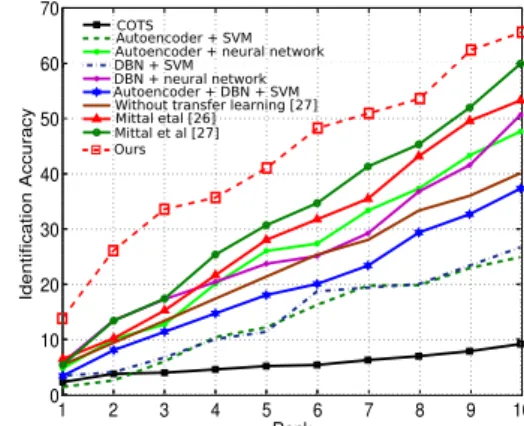
Faces(In) IdentiKit(As) Bhatt et al . [1] 24.0 ± 3.4 15.4 ± 3.1 Mittal et al . [16] 53.3 ± 1.4 45.3 ± 1.5 Mittal et al . [17] 60.2 ± 2.9 52.0 ± 2.4 Ours 65.6 ± 3.7 51.5 ± 4.0 1 2 3 4 5 6 7 8 9 10 0 10 20 30 40 50 60 70 Rank Identification Accuracy COTS Autoencoder + SVM Autoencoder + neural network DBN + SVM
DBN + neural network Autoencoder + DBN + SVM Without transfer learning [27] Mittal et al [27]Mittal etal [26]
Ours
Fig. 3. Rank-10 identification accuracy on the e-PRIP composite sketch database (left), and CMC curve for the Faces(In) database (right) for our result reported in the table.
In Figure 3 (left panel) we compare our results to the state of the art on the e-PRIP dataset. We obtain the best performance on the Faces(In) sketches, outperforming the previous state-of-the-art result of Mittal et al . [17] by 5%. For the IdentiKit(As) sketches our results are on par with those reported by Mittal et al . [17]. In Figure 3 (right panel) we plot the CMC curve for our method compared to the existing approaches on Faces(In) dataset, curves for other methods are taken from [17]. The figure shows that we obtain significant gain at all ranks compared to the state of the art.
5
Conclusion
We studied different aspects of leveraging a CNN pre-trained on visible spectrum im-ages for heterogenous face recognition, including extracting features from different CNN layers, finetuning the CNN, and using various forms of metric learning. We eval-uate the impact of these design choices via means of extensive benchmark results on different heterogenous datasets. The results we obtained are competitive with the state of the art for CASIA-NIR, and improve the state of the art on e-PRIP.
References
1. Bhatt, H.S., Bharadwaj, S., Singh, R., Vatsa, M.: Memetically optimized MCWLD for matching sketches with digital face images. Transactions on Information Forensics and Se-curity 7(5), 1522–1535 (2012)
2. Crowley, E., Parkhi, O., Zisserman, A.: Face painting: querying art with photos. In: BMVC (2015)
3. Fernando, B., Habrard, A., Sebban, M., Tuytelaars, T.: Unsupervised visual domain adapta-tion using subspace alignment. In: ICCV (2013)
4. Guillaumin, M., Verbeek, J., Schmid, C.: Is that you? Metric learning approaches for face identification. In: ICCV (2009)
5. Huang, G., Ramesh, M., Berg, T., Learned-Miller, E.: Labeled faces in the wild: a database for studying face recognition in unconstrained environments. Tech. Rep. 07-49, University of Massachusetts, Amherst (2007)
6. Jin, Y., Lu, J., Ruan, Q.: Large margin coupled feature learning for cross-modal face recog-nition. In: International Conference on Biometrics (2015)
7. Juefei-Xu, F., Pal, D., Savvides, M.: NIR-VIS heterogeneous face recognition via cross-spectral joint dictionary learning and reconstruction. In: Computer Vision and Pattern Recog-nition Workshops (2015)
8. Klare, B., Li, Z., Jain, A.: Matching forensic sketches to mug shot photos. PAMI 33(3), 639–646 (2011)
9. Kong, S., Heo, J., Abidi, B., Paik, J., Abidi, M.: Recent advances in visual and infrared face recognition – a review. CVIU 97(1), 103 – 135 (2005)
10. K¨ostinger, M., Hirzer, M., Wohlhart, P., Roth, P., Bischof, H.: Large scale metric learning from equivalence constraints. In: CVPR (2012)
11. Li, S., Yi, D., Lei, Z., Liao, S.: The CASIA NIR-VIS 2.0 face database. In: Computer Vision and Pattern Recognition Workshops (2013)
12. Lu, J., Liong, V., Zhou, X., Zhou, J.: Learning compact binary face descriptor for face recog-nition. PAMI (2015)
13. Martinez, A., Benavente, R.: The AR face database. Tech. rep. (1998)
14. Mignon, A., Jurie, F.: CMML: a new metric learning approach for cross modal matching. In: ACCV (2012)
15. Mignon, A., Jurie, F.: PCCA: A new approach for distance learning from sparse pairwise constraints. In: CVPR (2012)
16. Mittal, P., Jain, A., Goswami, G., Singh, R., Vatsa, M.: Recognizing composite sketches with digital face images via ssd dictionary. In: International Joint Conference on Biometrics (2014)
17. Mittal, P., Vatsa, M., Singh, R.: Composite sketch recognition via deep network-a transfer learning approach. In: International Conference on Biometrics (2015)
18. Parkhi, O., Vedaldi, A., Zisserman, A.: Deep face recognition. In: BMVC (2015)
19. Patel, V., Gopalan, R., Li, R., Chellappa, R.: Visual domain adaptation: a survey of recent advances. IEEE Signal Processing Magazine 32(3), 53 – 69 (2015)
20. Sarfraz, M., Stiefelhagen, R.: Deep perceptual mapping for thermal to visible face recogni-tion. In: BMVC (2015)
21. Schroff, F., Kalenichenko, D., Philbin, J.: Facenet: A unified embedding for face recognition and clustering. In: CVPR (2015)
22. Simonyan, K., Parkhi, O., Vedaldi, A., Zisserman, A.: Fisher vector faces in the wild. In: BMVC (2013)
23. Taigman, Y., Yang, M., Ranzato, M., Wolf, L.: DeepFace: Closing the gap to human-level performance in face verification. In: CVPR (2014)
8 Shreyas Saxena and Jakob Verbeek
24. Weinberger, K., Saul, L.: Distance metric learning for large margin nearest neighbor classi-fication. JMLR 10, 207–244 (2009)
25. Yi, D., Lei, Z., Liao, S., Li, S.: Learning face representation from scratch. In: Arxiv preprint (2014)
26. Yi, D., Lei, Z., Li, S.Z.: Shared representation learning for heterogeneous face recognition. In: International Conference on Automatic Face and Gesture Recognition (2015)