Improving LiDAR Point Cloud Classification using Intensities and Multiple Echoes

HAL Id: hal-01182604

https://hal.archives-ouvertes.fr/hal-01182604

Submitted on 3 Aug 2015

HAL is a multi-disciplinary open access

archive for the deposit and dissemination of

sci-entific research documents, whether they are

pub-lished or not. The documents may come from

teaching and research institutions in France or

abroad, or from public or private research centers.

L’archive ouverte pluridisciplinaire HAL, est

destinée au dépôt et à la diffusion de documents

scientifiques de niveau recherche, publiés ou non,

émanant des établissements d’enseignement et de

recherche français ou étrangers, des laboratoires

publics ou privés.

Improving LiDAR Point Cloud Classification using

Intensities and Multiple Echoes

Christophe Reymann, Simon Lacroix

To cite this version:

Christophe Reymann, Simon Lacroix. Improving LiDAR Point Cloud Classification using Intensities

and Multiple Echoes. IEEE/RSJ International Conference on Intelligent Robots and Systems (IROS

2015), Sep 2015, Hamburg, Germany. 7p. �hal-01182604�

Improving LiDAR Point Cloud Classification

using Intensities and Multiple Echoes

Christophe Reymann

and Simon Lacroix

Abstract— Besides precise and dense geometric information, some LiDARs also provide intensity information and multiple echoes, information that can advantageously be exploited to enhance the performance of the purely geometric classification approaches. This information indeed depends on the physical nature of the perceived surfaces, and is not strongly impacted by the scene illumination – contrary to visual information. This article investigates how such information can augment the precision of a point cloud classifier. It presents an empirical evaluation of a low cost LiDAR, introduces features related to the intensity and multiple echoes and their use in a hierarchical classification scheme. Results on varied outdoor scenes are depicted, and show that more precise class identification can be achieved using the intensity and multiple echoes than when using only geometric features.

I. INTRODUCTION

Identifying the various elements that constitute a scene is a primal concern for autonomous robots that navigate outdoors, be it simply to find feasible paths by identifying traversable areas, or more ambitiously to interpret and anal-yse the environment. The advent of LiDARs (LIght Detection And Ranging, [1]) has considerably eased the problem of scene classification and terrain traversability assessment. By providing at high rate dense range information that span large fields of view, such sensors allow the development of var-ious classification schemes that not only extract traversable areas (i.e. rather horizontal and smooth [2]), but also other elements (trees, cars, walls, etc.) that are present in the environment [3], [4].

But geometry alone may not be sufficient to assess the nature of some perceived elements. The physical nature of a flat ground impacts its traversability: hard concrete flat grounds are for instance very different from loose sand from this point of view – not to mention mud ponds. Similarly, blob shaped bushes are hardly distinguishable from boulders using only geometric information. Visual appearance, e.g. as captured by color or texture features, can help to assess this physical nature, and a vast amount of contributions in the vision and robotics literature deal with visual scene interpretation (e.g. [5]).

Besides distances, most time of flight LiDARs provide in-tensityinformation (also referred to as remission, reflectance, or amplitude). It measures the amount of reflected light, and is much less dependant on the scene illumination conditions than the intensities perceived by passive cameras. Also, since 1_{CNRS, LAAS, 7 avenue du colonel Roche, F-31400 Toulouse, France} 2_{Univ de Toulouse, UPS, LAAS, F-31400 Toulouse, France}

3_{Univ de Toulouse, LAAS, F-31400 Toulouse, France}

(christophe.reymann), (simon.lacroix) at laas.fr

LiDAR beams have a few cm width and a small divergence, some beams illuminate various points in the scene located a different depths, yielding multiple echoes.

The objective of this work is to assess to what extent the information conveyed by multiple echoes and intensity can improve the performance of range-only scene classification. The next section summarizes the basics of LiDAR distance and intensity measurements, and briefly reviews the literature dealing with the interpretation of LiDAR intensity informa-tion. Section III depicts the experimental characterization of a low-cost Hokuyo LiDAR1 _{that returns up to three echoes,}

so as to assess the scene parameters that affects the intensity measure. Section IV then presents the features used for the supervised classification process. Results are presented in section V, and a discussion concludes the article.

II. RELATED WORK

A. Background

The term LiDAR embraces the techniques that rely on measuring photons emitted by a laser and backscattered to the receiver. Most often, laser range finders used for airborne sensing or robotic applications rely on measuring the time of flight of the backscattered photons of a pulse of coherent light, so as to infer the range of obstacles.

Full-waveform LiDARs record the power of the backscat-tered pulse as a function of time, Pr(t), and output this

function as a discretized vector [6] (figure 1). Single-echo or multi-echo range finders operate according the same prin-ciple, but the Pr(t) function is internally processed to extract

one or multiple echoes corresponding to peaks, the distance of the scene points that generate them being derived by the associated time-of-flight t. The intensity associated to these echoes that corresponds to the proportion of backscattered energy is sometimes provided.

In [7], this received power function Pr(t) is modeled for

echoes on N Lambertian targets as: Pr(t) = D2ηsysρmcosα N X i=1 exp(−2Ria) 4R2 i Pe(t) (1)

where t denotes time, Pe the emitted power, D the aperture

diameter of the receiver optics, ηsys a system constant, Ri

the range of the ith obstacle, a the atmospheric attenuation coefficient, ρm the reflectivity of the surface and α the

incidence angle of the beam to the surface.

For robotic applications where distances do not exceed a few dozens of meters, the atmospheric attenuation is

Fig. 1. Transmitted and received power Pr(t) for a vertical laser beam

going through a tree – excerpt from [6].

negligible in clear conditions: the returned intensity then only depends on the surface reflectivity and is proportional to the inverse of the range squared. For purely Lambertian surfaces, the returned intensity is proportional to the cosine of the angle of the beam to the surface normal. But in the general case, the backscattered power is determined by the Bidirec-tional Reflectance Distribution Function, which is defined by the beam interactions with the surface. These interactions encompass subsurface scattering, diffusion, reflection and absorption, and can hardly be modelled for the variety of surfaces a robot can encounter.

Finally, lasers beams have a Gaussian profile with a small but non negligible angular spread: the beam footprint grows linearly with the distance. This affects the precision of the range estimate, which becomes dependant on the target distance, and also impacts the returned intensity.

B. LiDAR intensity interpretation

LiDAR intensity has mostly been used in airborne sensing, where full-waveform LiDARs are for instance used to clas-sify urban areas (e.g. by distinguishing grounds, buildings and vegetation [8]), or to discriminate vegetation from bare ground.

Much less work on the interpretation of LiDAR intensities and multiple echoes can be found in the robotics literature. This can be explained by the fact that full-waveform LiDAR are not widespread on ground vehicles, and that most of robotics-oriented LiDAR do not provide multiple echoes or calibrated intensities. Intensity values returned by most commercial single echo LiDARs are indeed hardly inter-pretable because of an adaptive gain control of the emitted power, or because no information is provided as to the quantization of the returned intensity. Lastly, as opposed to airborne sensing, ground based LiDARs generate data that span a large range of depths, with large variations of beam incidences on perceived objects, which strongly influence the measured intensity.

One of the first use of LiDAR intensity values in robotics is road marking detection. In [9], the authors build a 5 cm resolution raster map of the flat areas of an urban

environment that encodes the reflectivity. They augment a localisation process by correlating perceived and mapped reflectivities, which is eased by the high reflectivity of road markings. Other contributions focus on classifying roads surfaces from grass patches for navigation purposes, mostly in urban environments. In [10], the authors are able to distinguish flat grass areas from concrete or asphalt, by adding the intensity values to the 3D features in a learning scheme and update a probabilistic 2D grid model. The authors exploit a self-supervised learning technique using the vibrations measured on-board, and restrict the classification process to these two well separated classes. In [11], the authors fit a Gaussian mixture model on the histogram of calibrated intensity. Thresholds are then used to separate asphalt from grass. More recently, authors in [5] use LiDAR data (including intensity) fused with RGB data projected onto a grid to perform classification. Results are further improved and smoothed using conditional random fields. Authors in [12] perform segmentation of an urban scene in super-voxels, and show that adding features derived from LiDAR intensity improve classification scores. To our knowledge, only [13] used multiple echoes to detect vegetation in urban scenes from a full-waveform ground LiDAR. The authors extract regions containing multiple echoes, which are then classified using geometric features as vegetation and clutter. Regions that do not contain multiple echoes are always labeled as non-vegetation.

Besides classification, [14] compares LiDAR intensity images to camera images for the purpose of extracting keypoints for localisation and mapping. The former are shown to perform better, due to a lesser variability of the LiDAR intensity with respect to scene illumination and point of view.

III. EMPIRICAL CHARACTERISATION

To generate 3D scans, we use a Hokuyo UTM-30-LX-EW 2D LiDAR mounted on a tilt control unit. The LiDAR scans horizontally a 270◦ field of view at 40 Hz, with an angular resolution of 0.25◦, and returns up to three echoes for each measurement point. The light source has a wavelength of 905 nm, and no adaptive gain control is used for the emission – hence the return intensity of each echo only depends on the impacted surfaces distance, orientation and physical nature2. The beam divergence is not documented: using a near-infrared camera to measure the beam width at various distances, we assessed it as equal to 1 mRad, a usual value for most LiDARs.

A. Intensities

Figure 2 shows the intensity measurements at 0◦incidence angle as a function of the distance for various materials. Up to a distance of approximately 0.8 m, the measurements do not fit at all the model: this phenomenon is often referred to as the “near distance effect”, which can be due to the fact that the emitter and the receiver are not strictly aligned,

or to the fact that the receiver optics does not focus well for such distances [15]. For further distances, the intensity then decreases proportionally to the inverse of the squared distance, according to eq. (1).

2 3 4 5 6 7 8 9 0 1 2 3 4 5

Intensity (no unit)

Range (m) cardboard black chair white pane green foam steel sheet

Fig. 2. Intensity (scaleless values) as a function of the distance in m for various materials. The black curve is the fit of a squared inverse function on white pane data ranges > 1 m.

Figure 3 shows the evolution of the measured intensity as a function of the incidence angle (10 measures are taken for each angle value). Wood is mostly Lambertian: the reflected intensity follows a cosine law, as expected by eq. (1).

2.6 2.8 3 3.2 3.4 3.6 0 10 20 30 40 50 60 70

Intensity (no unit)

Angle (deg)

wood

Fig. 3. Intensity (scaleless values) reflected by a wood pane as a function of the angle in degrees.

B. Multiple echoes

To analyze multiple echoes, beams that impact on two white panes located at different distances have been recorded. We used the tilt unit to achieve a fine angular resolution. Figure 4 shows typical results: for depth gradients smaller than 0.5 m, the LiDAR cannot separate properly the two surfaces and produces distances in between the surfaces that have no physical meaning, probably because the echo fitting averages the two intensity peaks. As the depth gradient grows, second echoes appear and the surfaces are well

separated3_{. As expected, there is a direct correlation between}

the area of the spot on the surface and the returned intensity: the fraction of the beams intensity returned by the first echo decreases as the intensity of the second echo increases. This expected behavior can help to precisely locate edges that correspond to depth gradients, as done in [16].

-0.06 -0.05 -0.04 -0.03 -0.02 -0.01 0 1.5 1.55 1.6 1.65 1.7 1.75 y (m) x (m) 1st echo 3.6 3.8 4 4.2 4.4 4.6 4.8 5 -0.12 -0.1 -0.08 -0.06 -0.04 -0.02 0 1.5 2 2.5 3 3.5 y (m) x (m) 1st echo 2nd echo first-second echo vector

0 0.1 0.2 0.3 0.4 0.5 0.6 0.7 0.8

Fig. 4. Visualisation of multiple echos for two different depth gradients. Top: with a 0.25 m depth gradient, no second echoes are generated (the points color indicate their intensity), and for the few beams that intersect the two surfaces, wrong distance measurements are returned. Bottom: for a 1.5 m depth gradient, several multiple echoes are returned for the beams that impact both surfaces. Second echoes are plotted in green, and a line is drawn for each returned pair of echoes, with a color that represents the intensity of the first echo divided by the sum of intensities of the first and second echoes.

C. Synthesis

These empirical measures suggest that the intensity in-formation provided by our Hokuyo range finder could be used to distinguish various surfaces, at least up to a few meters (figure 2). But unfortunately, the decorrelation of the intensity value from the incidence angle and the range does not seem tractable for complex outdoor scenes, as each surface behaves in a different way, and only a few can be reasonably assumed Lambertian. Therefore range 3_{Third echoes are very scarce, and occur on natural scenes only for a}

and incidence should be used in combination with intensity returns for classification, but this raises two issues. First, the incidence angle can only be estimated on planar patches in the 3D scan – it can not on vegetation for instance. Second, obtaining a good learning set that covers all the combinations of these three values is hardly tractable for all possible surfaces.

For depth gradient smaller than 0.5 m, our LiDAR is un-able to separate multiple echoes, which results in a measure corresponding to an in-between depth. Echoes are well sepa-rated for higher depth gradients, but the associated intensities then depend on the proportion of the beam that generate the echo. Hence the intensity should not be considered for the classification of multiple echoes.

IV. POINT CLOUD CLASSIFICATION

To generate a 3D voxel-based model of the environment, we use the Hokuyo LiDAR mounted on a tilt unit on a mobile robot, and process the point clouds generated by a scan acquired while the robot is at rest4. Each gathered point cloud contains a maximum number of points of about 200,000, and is sub-sampled in voxels of size Sv using octrees from the

PCL implementation [17]. A feature vector is then computed for each occupied voxel over its neighborhood, defined by the ball of radius Rs > Sv centered on the voxel. This

voxelisation is conducted in order to subsample the point cloud and therefore drastically reduce the the classification runtime. It is fairly well adapted for robotic application were a finer level of detail is not needed, and fast online processing is of utter importance.

A. Geometric features

A principal component analysis on the Euclidean coordi-nates of the points contained in each voxel neighborhood is applied. The vector associated to the smallest eigenvalue is kept as the surface normal estimate. Three features p0, p1

and p2 are computed from the eigenvalues e1, e2, and e3

(e1> e2> e3) as follows:

p0= (e1− e2)/e1 ; p1= (e2− e3)/e1 ; p2= e3/e1 (2)

These features capture the shape of the neighboring points: if p0= 1 the points are distributed on a line, if p1= 1 they

are on a plane and if p2= 1 they are evenly scattered along

the 3 directions [18]. Two additional features are derived from the normal vector estimate: the angle θ between the normal and the vertical, and the incidence angle αI between

the normal and the “view line” that links the voxel centroid to the LiDAR origin. The first one disambiguates ground from verticals, and the second conditions the intensity values. B. Intensity features

Two intensity-related features are defined: the mean intensity µI and the intensity standard deviation σI of the

4_{The tilt resolution is set to 0.25}◦_{, similar to the angular resolution of}

the LiDAR, so that the angular resolution of the point cloud is regular in both pan and tilt directions.

points in the voxel’s neighborhood. For these features, only points that don’t have associated multiple echoes are used, to avoid the caveats described in section III-C.

The mean range µρ of the neighborhood points is also

used, as it conditions the intensity features along with the in-cidence angle αI, as we did not calibrate intensity values (see

section III-C). The range and incidence angle features may introduce erroneous results during classification, as these features are not representative of the surface, but depend on the way they are perceived. Making sure each class of the learning set is perceived over the whole range of these features is nearly impossible for all classes. Therefore they must only be used when necessary and only to discriminate amongst classes perceived over the same combinations of distances and incidence angles to avoid this bias (see section IV-E).

C. Multi-echo features

Multiple echoes are caused by significant depth gradients, and occur in two cases: at the edge of obstacles (walls, trees, fences), and in cluttered areas, typically tree leaves or tall grass. Obstacles have clearly cut edges, and for multiple echoes returns, the first echoes returns appear along lines or contours (e.g. for walls or trees) or on a plane (e.g. wire fences). Whereas in the case of vegetation or tall grass, they appear in a more scattered manner. In order for the multiple echoes to be discriminative, the voxel neighborhood size should be set in relation with the details one wish to capture. Points to which a second (or third) echo is associated are considered apart from the others (which in turn allows not to corrupt the intensity features of the other points), and the geometric features presented in section IV-A are computed. Additionally, the proportion of these points is added to the voxel feature vector.

One issue with multi-echo features is that the proportion of points that have secondary echoes is low, reaching at most 20% in our experiments, and thus these features are all equal to zero in most voxels. Even for classes that should contain a lot of multiple echoes (such as tall grass), a non negligible voxel proportion does not contain multiple echoes – again the size of the voxel’s neighborhood matters here.

D. Supervised learning

We use a Random Forest classifier, as it has shown to fare well for point cloud data, yielding good probabilities estimates [19]. Classification was implemented in Python using the scikit-learn toolkit5_.

We selected a set of six classes relevant to the navigation task and the considered urban and natural environments: short grass, asphalt, small rocks/gravel, obstacle (wall, tree trunk...), dense vegetation (non drivable, e.g. trees or bushes) and sparse vegetation (drivable, e.g. tall grass). Our first objective is to be able to distinguish seemingly flat surfaces

(short grass, asphalt and small rocks) from each other by taking advantage of the intensity information. A secondary objective is to exploit multi-echo features to enhance classi-fication of non-flat but driveable terrain such as tall grass. E. Hierarchical Classification

Due to their nature, intensity and multi-echo information are only relevant to separate some classes. Using all these features as input for a classifier may be counter-productive, as it would introduce a bias for classes for which they are not relevant (for example, using intensity information for clas-sifying walls only make sense when one wants to separate different types of walls). It could even be detrimental to the classification: a bush could return a intensity value very close to that of a piece of wall, and induce misclassifications that would not happen considering only geometric features. We therefore introduced a very simple handcrafted hierarchical classification process inspired from SVM Decision Trees (SVMDT) used in [20]: a decision tree is defined, with a classifier at each node that only uses a subset of the available features. Each node classifies the data in a subset of the remaining labels.

Using only geometric features, the root node classifies the data into three categories: flat surfaces (grass, asphalt, rocks), obstacles, and vegetation (dense and sparse). Flat surfaces are further refined using only intensity related features, and vegetation classes are refined using geometric, multi-echo and intensity features.

V. EXPERIMENTS

A. Methodology

We acquired data in three different locations: in a parking lot, around a small water pond, and on an abandoned sport field. The perceived scenes include trees, bushes, rocks, fences, and tall grass that would be considered as not drive-able by a purely geometric interpretation of the data. A set of eighteen scans were labelled by hand, the breakdown of the number of samples for each class is shown in table I. In total about 17000 sample voxels were used to define a training and validation set. We set the voxel size to 15cm and the voxel neighborhood radius to 30cm. These values were selected after trials and errors: increasing voxel (and neighborhood) size allows for more multiple echoes in voxels, but decreases the accuracy of classification on surface boundaries. To ensure the computed features are significant, we introduced a threshold on the number of points per voxel (set to 5 in our experiments), under which voxels are not classified. A greater value did not provide better performances and left out too many voxels thus impacting negatively the depth of view (note that the minimum threshold value is 3, under which it is not possible to compute geometric features).

The classifiers have been trained with the manually labeled scans, using 200 estimators for the random forest classifier – training it with more estimators did not improve the results. So as to assess the relevance and influence of the different categories of features, we conducted stratified 3-fold cross-validation on the training set. First we did so using

Label #Samples Percentage Short Grass 4195 25 Asphalt 4230 25 Small rocks 862 5 Obstacle 2411 14 Dense vegetation 2127 13 Sparse vegetation 2947 18

TABLE I. Number of voxel samples and distribution of each label in the training dataset.

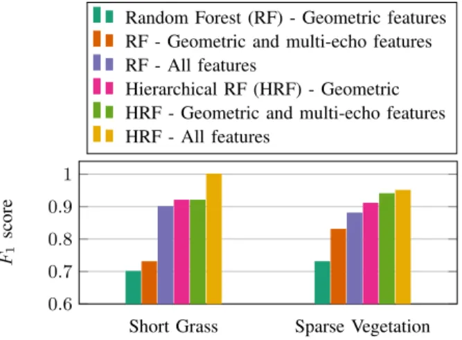
Short Grass Sparse Vegetation 0.6 0.7 0.8 0.9 1 F1 score

Random Forest (RF) - Geometric features RF - Geometric and multi-echo features RF - All features

Hierarchical RF (HRF) - Geometric HRF - Geometric and multi-echo features HRF - All features

Fig. 5. Excerpt from table II: F1 score comparison for Short Grass and

Sparse Vegetation after 3-fold cross-validation.

only geometric features, then using all features, on both the Random Forest classifier and the hierarchical version defined in section IV-E. The F1 score is used to assess the quality

of the classification: F1= 2 ×

precision × recall

precision + recall (3)

It summarizes the precision and recall scores in a way that puts the emphasis on having both of them as high as possible (F1 = 0 if either precision or recall is equal to

zero, and F1= 1 implies that both precision and recall are

equal to one). The F1score results are compiled in table II.

B. Results

Label R,G R,GM R,All H,G H,GM H,All Short Grass 0.70 0.73 0.90 0.92 0.92 1.00 Asphalt 0.86 0.86 0.97 0.95 0.95 1.00 Small rocks 0.24 0.31 0.73 0.80 0.80 0.97 Obstacle 0.91 0.91 0.89 0.94 0.94 0.94 Dense veg. 0.62 0.73 0.83 0.83 0.87 0.92 Sparse veg. 0.74 0.83 0.88 0.91 0.94 0.95 Average 0.75 0.79 0.89 0.91 0.91 0.97 TABLE II. Comparison of F1 scores for each label after 3-fold

cross-validation using random forest or the hierarchical version, using geometric features only or using all features. R = Random Forest classifier, H = Hierarchical scheme with Random Forest classifier, All = all features, G = only geometric features, GM = geometric and multi-echo features. The average scores over all classes are computed taking into account number of samples for each class.

Overall, the Random Forest classifier fares well: using all features, it is able to distinguish grass, asphalt and small rocks, three surfaces that are very similar from a pure geometric point of view. The F1 score for short grass and

small rocks respectively raises from 0.7 to 0.9 and 0.24 to 0.73 when using all features instead of only geometric ones. Scores for dense and sparse vegetation are also improved using all the features. But on the contrary, geometric features suffice to label obstacles as such: adding intensity features is detrimental and slightly degrades performances, lowering F1 from 0.91 to 0.89. On the Random Forest classifier,

using multi-echo features slightly improves performances on ground classes as it prevents misclassification between them and vegetation.

The results are much improved when using the hierarchical classification scheme, even when using only geometrical features at each node (see the “H,G” column): flat surfaces are often more precisely identified than when using Random Forest with all features, and dense and sparse vegetation are also better separated. It is due to the fact that the classifier is better at separating classes that are geometrically very dif-ferent. Indeed the root node separates ground, obstacles and vegetation using purely geometrical features, and therefore is not polluted by intensity features that sometimes match between groups.

The use of intensity features in the hierarchical scheme improves even more the results. As compared to the classic Random Forest scheme with all attributes, the score for small rocks raises up from 0.80 to 0.97 and short grass and asphalt are almost perfectly classified. Finally, multi-echo features are beneficial for the classification of vegetation, slightly improving the score of sparse vegetation from 0.91 to 0.94 and of dense vegetation from 0.83 to 0.87 : they help discrim-inate amongst these two classes. Although the improvement is small in value, one should take into consideration the limitations of the sensors, which generates only very few multiple echoes in sparse vegetation environments such as tall grasses.

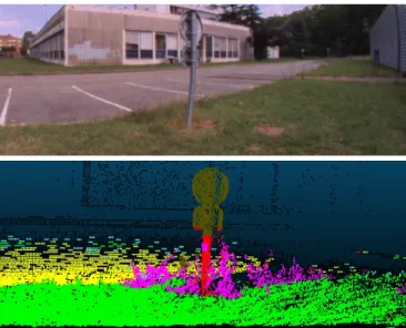
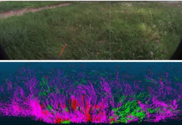
Figures 6 to 9 show illustrative examples of classified point clouds, along with a picture of the scene (taken with a camera equipped with a fish-eye lens, whose perspective does not exactly match the one of the point clouds). Note that these scenes are more complex than the one used for the training set: to ease manual labelling and properly initiate the learning phase, the training scenes were indeed chosen so as to be easily segmented and labeled.

As expected, labels assigned on structures and surfaces that were not part of the learning process are not well identified: in figure 6 and 8 boardwalk borders and car angles are sometimes classified as rock (the intensity values returned by the concrete must be very close of those of rocks), sometimes as vegetation (certainly because the voxel neighborhood radius is greater than the size of the step, and thus the computed p2 feature value is abnormally high). In

fig. 8, the asphalt is somewhat worn out. As the classifier was trained using asphalt of better quality, it misclassifies some parts of it as rock. The weaker spot is vegetation. In fig. 7

the road sign base is classified as dense vegetation, because it is surrounded by tall grass (the corresponding voxels also contain some grass blades). And when the robot is surrounded by tall grass as in fig. 9, the classifier labels some tall grass clumps as dense vegetation. It happens particularly often for the nearest ones, as they are less likely to generate multiple echoes. Finally, fig. 7 illustrates a last issue: for points laying too far on the ground, wrong classifications can occur as a result of lower separability of the intensities (see section II-B) and lower precision of the angle of incidence.

Fig. 6. Classification results with hierarchical Random Forest scheme on a scan taken in a parking lot. Top: view of scan location taken with a fish-eye lens. Bottom: classified point cloud of the location, with point colors corresponding to labels as follows: green/short grass, yellow/asphalt, light blue/rocks, brown/obstacles,pink/sparse vegetation, red/dense vegetation and no label/black.

Fig. 7. Classification results with hierarchical Random Forest scheme on an other parking lot (same color codes as in figure 6).

VI. DISCUSSION ANDCONCLUSION

This paper investigated the use of intensity and multiple echoes information to help the classification of outdoor LiDAR point clouds. Results are preliminary, but go further than previous work in robotics. They show that even for com-plex scenes and with a low-cost LiDAR, the consideration of

Fig. 8. Classification results with hierarchical Random Forest scheme on an old asphalt road (same color codes as in figure 6).

Fig. 9. Classification results with hierarchical Random Forest scheme on an abandoned football field with patches of tall grass (same color codes as in figure 6)

these information leads to finer classification – even though the discriminant power of the intensity drastically decreases with the distance. Multiple echoes have little impact on the classification: this is certainly due to the fact that the sensor can not separate echoes for depth gradients smaller than 0.5 m. This is an important limiting factor when navigating in dense environment such as tall grass, which would be alleviated by a more precise sensor.

Because of the dependence on range and orientation, one must be careful in using intensity features so that they do not introduce an unwanted bias on classes where this information is not relevant. This bias can be mitigated by introducing a hierarchical classification scheme, where classes are refined recursively using different subsets of features at each step. This way subsets of features can be tailored to fit the nature of the desired discrimination, as we did by first isolating mostly planar ground surfaces from the rest using only geometric features, and then refining the generic class by using intensity features. In future work such a decision tree that implies feature selection could be learned directly from the data in an unsupervised manner.

REFERENCES

[1] P. F. McManamon, “Review of ladar: a historic, yet emerging, sensor technology with rich phenomenology,” Optical Engineering, vol. 51, no. 6, 2012.

[2] P. Papadakis, “Terrain traversability analysis methods for unmanned ground vehicles: A survey,” Engineering Applications of Artificial Intelligence, vol. 26, no. 4, pp. 1373–1385, 2013.

[3] J.-F. Lalonde, N. Vandapel, D. F. Huber, and M. Hebert, “Natural terrain classification using three-dimensional ladar data for ground robot mobility,” Journal of Field Robotics, vol. 23, no. 10, pp. 839– 861, 2006.

[4] B. Douillard, J. Underwood, N. Kuntz, V. Vlaskine, A. Quadros, P. Morton, and A. Frenkel, “On the segmentation of 3D LIDAR point clouds,” in 2011 IEEE International Conference on Robotics and Automation. IEEE, 2011, pp. 2798–2805.

[5] S. Laible, Y. N. Khan, and A. Zell, “Terrain classification with conditional random fields on fused 3D LIDAR and camera data,” in 2013 European Conference on Mobile Robots (ECMR). IEEE, 2013, pp. 172–177.

[6] C. Mallet and F. Bretar, “Full-waveform topographic lidar: State-of-the-art,” ISPRS Journal of Photogrammetry and Remote Sensing, vol. 64, no. 1, pp. 1–16, Jan. 2009.

[7] C. Mallet, “Analyse de donn´ees lidar `a Retour d’Onde Compl`ete pour la classification en milieu urbain,” Ph.D. dissertation, Telecom ParisTech, 2010.

[8] L. Guo, N. Chehata, C. Mallet, and S. Boukir, “Relevance of airborne lidar and multispectral image data for urban scene classification using Random Forests,” ISPRS Journal of Photogrammetry and Remote Sensing, vol. 66, no. 1, pp. 56–66, Jan. 2011.

[9] J. Levinson, M. Montemerlo, and S. Thrun, “Map-Based Precision Vehicle Localization in Urban Environments,” in Robotics: Science and Systems, 2007.

[10] K. M. Wurm, R. K¨umerle, C. Stachniss, and W. Burgard, “Improving Robot Navigation in Structured Outdoor Environments by Identifying Vegetation from Laser Data,” in IEEE/RSJ International Conference on Intelligent Robots and Systems (IROS), St. Louis, USA, October 11-15 2009.

[11] T. Saitoh and Y. Kuroda, “Online Road Surface Analysis using Laser Remission Value in Urban Environments,” in IEEE/RSJ International Conference on Intelligent Robots and Systems (IROS), Taipei, Taiwan, October 18-22 2010.

[12] A. K. Aijazi, P. Checchin, and L. Trassoudaine, “Segmentation based classification of 3d urban point clouds: A super-voxel based approach with evaluation,” Remote Sensing, vol. 5, no. 4, pp. 1624–1650, 2013. [13] J. Elseberg, D. Borrmann, and A. Nuechter, “Full Wave Analysis in 3D laser scans for vegetation detection in urban environments,” in Information, Communication and Automation Technologies (ICAT), Sarajevo, Bosnia and Herzegovina, October 27-29 2011.

[14] C. McManus, P. Furgale, and T. Barfoot, “Towards appearance-based methods for lidar sensors,” in Robotics and Automation (ICRA), 2011 IEEE International Conference on, May 2011, pp. 1930–1935. [15] W. Fang, X. Huang, F. Zhang, and D. Li, “Intensity correction

of terrestrial laser scanning data by estimating laser transmission function,” Geoscience and Remote Sensing, IEEE Transactions on, vol. 53, no. 2, pp. 942–951, Feb 2015.

[16] J.-C. Michelin, C. Mallet, and N. David, “Building Edge Detection Using Small-Footprint Airborne Full-Waveform Lidar Data,” in XXII ISPRS Congress, Melbourne (Australia), 2012.

[17] R. B. Rusu and S. Cousins, “3D is here: Point Cloud Library (PCL),” in IEEE International Conference on Robotics and Automation (ICRA), Shanghai, China, May 9-13 2011.

[18] N. Brodu and D. Lague, “3D terrestrial lidar data classification of complex natural scenes using a multi-scale dimensionality criterion: Applications in geomorphology,” ISPRS Journal of Photogrammetry and Remote Sensing, vol. 68, pp. 121–134, March 2012.

[19] A. Niculescu-Mizil and R. Caruana, “Predicting good probabilities with supervised learning,” in Proceedings of the 22nd international conference on Machine learning. ACM, 2005, pp. 625–632. [20] P. Krahwinkler, J. Rossmann, and B. Sondermann, “Support vector

machine based decision tree for very high resolution multispectral forest mapping,” in Geoscience and Remote Sensing Symposium (IGARSS), 2011 IEEE International, July 2011, pp. 43–46.