HAL Id: hal-01350068
https://hal.archives-ouvertes.fr/hal-01350068
Submitted on 29 Jul 2016
HAL is a multi-disciplinary open access
archive for the deposit and dissemination of
sci-entific research documents, whether they are
pub-lished or not. The documents may come from
teaching and research institutions in France or
abroad, or from public or private research centers.
L’archive ouverte pluridisciplinaire HAL, est
destinée au dépôt et à la diffusion de documents
scientifiques de niveau recherche, publiés ou non,
émanant des établissements d’enseignement et de
recherche français ou étrangers, des laboratoires
publics ou privés.
Deep complementary features for speaker identification
in TV broadcast data
Mateusz Budnik, Laurent Besacier, Ali Khodabakhsh, Cenk Demiroglu
To cite this version:
Mateusz Budnik, Laurent Besacier, Ali Khodabakhsh, Cenk Demiroglu. Deep complementary features
for speaker identification in TV broadcast data. Odyssey Workshop 2016, Jun 2016, Bilbao, Spain.
�10.21437/Odyssey.2016-21�. �hal-01350068�
Deep complementary features for speaker identification in TV broadcast data
Mateusz Budnik, Laurent Besacier
Laboratoire d’Informatique de Grenoble
Univ. Grenoble-Alpes
Grenoble, France
Ali Khodabakhsh, Cenk Demiroglu
Electrical and Computer Engineering Department
Ozyegin University
Istanbul, Turkey
[email protected] [email protected]
Abstract
This work tries to investigate the use of a Convolutional Neu-ral Network approach and its fusion with more traditional sys-tems such as Total Variability Space for speaker identification in TV broadcast data. The former uses spectrograms for training, while the latter is based on MFCC features. The dataset poses several challenges such as significant class imbalance or back-ground noise and music. Even though the performance of the Convolutional Neural Network is lower than the state-of-the-art, it is able to complement it and give better results through fusion. Different fusion techniques are evaluated using both early and late fusion.
1. Introduction
In the past few years, Convolutional Neural Networks (CNN) became widely used in image related domains providing state-of-the-art performance [1]. At the same time Deep Neural Net-works (DNN) were being applied more and more to mono-dimensional signals for tasks like language recognition [2], speech recognition [3] or speaker identification [4]. Lately, there was an increasing number of studies trying to address some of the related tasks (notably automatic speech recogni-tion) with the use of CNN based systems with only spectro-grams as input [5, 6]. However, such systems have not yet been widely explored for speaker identification. This study tries to give additional insight into the efficient use of CNN for this particular biometrics task.
Contribution In this paper, the use of convolutional neural networks (CNNs) for speaker identification is investigated. Ad-ditionally, a challenging dataset was selected, containing both noise and un-balanced speaker data. This CNN approach is compared to more traditional methods. Despite the lower CNN performance, the use of this deep complementary features in fusion improves on the state-of-the-art.
Outline The structure of this paper is as follows. Section 2 presents a short overview of the recent developments in connec-tion to this study. Secconnec-tion 3 gives the overview of the methods proposed. This is followed by the presentation of the experi-mental framework in Section 4. The results are presented in Section 5. Section 6 contains the concluding remarks.
2. Related Works
In [7] a speech recognition system is presented that uses raw speech as input, which is then processed by a 1D convolu-tional layer. The use of CNN with spectrograms was also ex-plored previously: in [8] a system dealing with phonetic
confu-sion is presented, however convolution is done only along the frequency axis. An interesting approach was presented in [9] where an unsupervised approach to feature learning is proposed. The algorithm is based on a convolutional deep belief network. Apart from that, Recurrent Neural Networks (RNN) were also successfully used with speech spectrograms, as it is suggested in [10] for automatic speech recognition.
An approach similar to this study is presented in [6]. In their paper, a CNN is trained using spectrograms in order to identify disguised voices. However, compared to our paper, this study considered a significantly smaller number of speakers with the explicit goal of identifying fraudulent behavior and different identities. In addition, no fusion approaches were explored. Apart from a more noiseless and balanced dataset, a different CNN architecture (based on AlexNet[11]) is also used. Con-versely, the base architecture used in our study is simpler and provides better performance [12].
Some attempts were also made to use CNNs in noisy condi-tions. A recent study [13] uses 1D convolutions on filter banks. Surrounding frames are taken into account and serve as context to reduce noise impact.
In [14], a study was done on emotion recognition by combi-nation of audio and visual features. Similar to this study, spec-trograms were used, and 1D and 2D CNNs were evaluated. In [5], CNNs were used for the language identification task. Fi-nally, speaker and language recognition experiments using neu-ral networks were also presented in [4].
3. Method description
3.1. Speaker Identification Systems
Gaussian Mixture Model-Universal Background Model
(GMM-UBM) [15] and Total Variability Space (TVS) [16] speaker recognition systems are used in this study.
In the GMM-UBM approach, a Universal Background Model (UBM) is first trained on speech features extracted from multiple speakers using the Expectation-Maximization (EM) algorithm. Speaker-specific models are then obtained using Maximum a Posteriori (MAP) mean adaptation. Similarity scoring is done by calculation of log-likelihood ratio (LLR) on these models. Given a sequence of feature vectors X ex-tracted from a test segment, LLR is computed as Λ(X) = log p(X|λhyp) − log p(X|λubm), where λhypand λubm
rep-resent speaker-specific GMM and UBM model respectively. After adaptation, models can also be represented as high-dimensional supervectors of means of distributions. These su-pervectors can be represented as low-dimensional identity
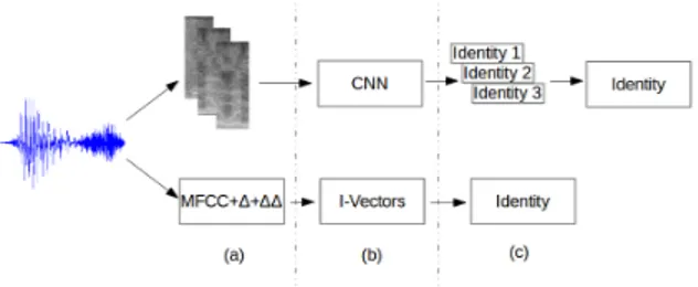
vec-Figure 1: A simplified overview of the system, which highlights how the convolutional neural network was used in this study in contrast to a more traditional approach.
tors (i-vector) using factor analysis. In this approach, mean supervectors Ms and M0 representing speaker-specific model
and UBM respectively are extracted, and an i-vector, ws, is
cal-culated using Ms = M0 + T ws. The low-rank rectangular
matrix, T , representing the variability space of the i-vectors, is learned in an unsupervised manner using the Expectation-Maximization (EM) algorithm. In the case of having multi-ple tracks for speaker modeling, i-vectors extracted from each speech track are typically averaged and the average i-vector is used as the speaker model. Scoring can be done with cosine similarity metric, while pre-processing i-vectors before scoring can result in better performance.
In our setup, speaker identification is done by scoring a test segment versus all the speaker models. The speaker identity corresponding to the highest similarity score is chosen as the result of the identification test.
A UBM consisting of 1024 gaussians is trained on the train-ing data for both systems. T matrix is then trained on the seg-mented training data. Segmentation outputs of conventional BIC-criterion [17] are used. The dimension of output i-vectors is set to 500. MSR Identity Toolbox [18] is used for all exper-iments. Similarity scoring is done by cosine similarity scoring between the test segment and the i-vector representing target identity. Similarity scoring is also done using probabilistic lin-ear discriminant analysis (PLDA) [19] for additional compari-son using the same toolkit. A wide range of different parame-ter values was tested to ensure the best possible performance. Length normalization [19] is used for increased performance. 3.2. Convolutional Neural Networks
In Figure 1 the general way in which the CNN algorithm is ap-plied can be seen. For any given speech segment (Fig. 1a) the spectrograms are first extracted. Because they have a fixed size there are usually several overlapping spectrograms representing each segment. Next (Fig. 1b) , each spectrogram is fed to the convolutional neural network separately. This in turn produces an individual vector of potential speaker identities for every in-put (Fig 1c). Finally, to obtain a single vector for the speech track, the individual vectors are averaged.
The network used in this study is inspired by the general design proposed in [12] for image recognition. It was chosen as a starting point due to its relative structure simplicity and state-of-the-art performance. However, several changes were made in order to adapt it to this specific speaker identification task. The significant differences between the ImageNet dataset (con-taining images of everyday objects and animals among others), on which the reference network was originally trained, and the spectrogram data made it necessary to retrain the whole
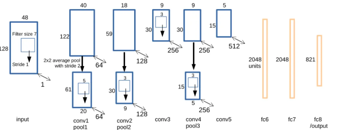
algo-rithm from scratch. Due to a less complex nature of the spec-trogram data (monochromatic with similar patterns) a reduced version of the original model was introduced with no visible change in performance. The detailed structure can be found in Table 1. The visualization of this network is shown in Figure 2.
name type filter size output size
/ stride
input: 48 × 128 grayscale image of spectro.
conv1 convolution 7 × 7/1 40 × 122 × 64
pool1 ave pooling 2 × 2/2 20 × 61 × 64
conv2 convolution 5 × 5/1 18 × 59 × 128
pool2 ave pooling 2 × 2/2 9 × 30 × 128
conv3 convolution 3 × 3/1 9 × 30 × 256
conv4 convolution 3 × 3/1 9 × 30 × 256
pool3 ave pooling 2 × 2/2 5 × 15 × 256
conv5 convolution 3 × 3/1 5 × 15 × 512
fc6 full conn 1 × 1 × 2048
fc7 full conn 1 × 1 × 2048
fc8 full conn 1 × 1 × 821
Table 1: The structure of the network.
The network was trained from scratch on a set of grayscale spectrogram images with non-square dimensions. The model was trained for around 12 epochs. Every convolutional layer was followed by a rectified linear unit (ReLU), which serves as an activation function and is defined as f (x) = max(0, x). The first two fully connected layers (fc6, fc7) are followed by ReLU and dropout with the rate of 0.5. The output of the last fully connected layer (fc8) is used with the softmax function and corresponds to the target speakers (821 individual speakers in total).
Different to the initial design for image recognition, the pro-posed structure has fewer convolutional layers (from 8 down to 5), however the filter size for the first two is expanded. Adding additional convolutional layers did not improve performance. Average pooling layers were chosen instead of max pooling. The input to the network is a 48 × 128 pixel grayscale image of a spectrogram. Due to the overlap between the images, no ran-dom cropping or rotation is used during training. Caffe frame-work [20] was used for training and testing the net.
The network gives predictions based on individual spectro-grams. In order to be able to fuse the output with the output of the TVS system, the spectrograms are mapped to bigger speech segments. The mapping is done by averaging the scores of ev-ery spectrogram contained within a given segment.
In Figure 3a an example of a spectrogram used for training is shown. Figure 3b represents the saliency map, i.e. a heatmap representing the most significant regions of the image used by the CNN to predict a given speaker. In this case it represents speaker with the highest response from the top layer. This was obtained by backpropagating the correct output from the last layer to the input layer in a similar way as it was done in [21]. Note the heavy reliance on horizontal patterns.
3.3. Fusion
Fusion is often used to enhance results for speaker recognition systems, for example in [13]. Even if by itself a system gives inferior results, it still can help to improve the baseline perfor-mance. In this article, several attempts were made to fuse the
1 64 64 128 128 256 256 256 512 48 128 40 122 20 61 18 59 9 30 9 30 9 30 15 5 15 5 2048 units 2048 821 Filter size 7 5 3 3 3
Stride 1 2x2 average poolwith stride 2
input conv1 pool1 conv4 pool3 conv3 conv2 pool2 conv5 fc6 fc7 fc8 /output
Figure 2: The visualization of the CNN used in this study. A spectrogram is taken as input and is convolved with 64 different filters (with the size of 7×7) at the first layer with the stride equal to 1. The resulting 64 feature maps are then passed through the ReLU function (not visible here) and downsampled using average pooling. A similar process continues up to the fully connected layers (f6, which takes conv5 as input, and fc7) and the final output layer (corresponding to the number of speakers in the train set).
(a) (b)
Figure 3: (a) An example of a spectrogram used in this study. (b) A saliency map representing the networks response to this spectrogram.
CNN results with the output of the TVS system. Both early and late fusions were considered.
3.3.1. Late Fusion
A conventional late fusion of normalized predictions taken from both systems was used, which is the average of the two outputs. A weighted sum of both outputs was also tested.
3.3.2. Duration-based Late Fusion
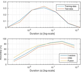
This strategy was proposed to give the CNN scores higher weights for short duration segments and lower ones for the long speech segments. CNN seems to produce comparable results to the TVS system on short segments, while the difference in per-formance grows with increasing duration. Fusion on the longer segments also seems to be less beneficial. This is illustrated in the bottom plot of Figure 5. In this case, fusion was calculated as s = (1 − tanh(d))scnn+ sivec, where s corresponds to the
scores provided by each system and d is the segment duration. 3.3.3. Early Fusion with Support Vector Machines
This strategy serves as early fusion, where a linear SVM is used for the final classification decision based on a concatenated nor-malized outputs of CNN’s last hidden layer and i-vectors. Prin-cipal component analysis is applied to the CNN output in order
to match the i-vector dimensionality (500 for each).
4. Experimental Setup
4.1. Dataset
The REPERE corpus [22] was used in this study. The dataset contains a set of videos from two French television channels (LCP and BFM). There are 7 types of videos, ranging from news shows, debates to celebrity gossip and culture programs. Only the audio track was used in the experiments.
The dataset is quite challenging. The recording takes place both inside a studio setting and outside in public and noisy en-vironments. Apart from this, music is often played in the back-ground during certain presentations or interviews. Addition-ally, there is a significant imbalance between speakers, with an-chors and top politicians both being often over-represented in the dataset. Total amount of speech per speaker for speakers present in both train / test sets helps to illustrate this and it is shown in Figure 4. Normalized histogram of the number of segments for each duration bin is also shown in Figure 5 for training and test data. It is important to mention that a big por-tion of speech segments fall below 2 seconds of speech. For the test set, 24.8% of speech segments are shorter than 2 seconds, and 70.4% are shorter than 10 seconds.
Experiments were done in a closed-set manner, where all the speakers in the training data are used for training mod-els, while performance is evaluated only on test segments from speakers overlapping between training and test data. There are 821 speakers available in the training data, from which only 113 are observed in the test data.
Training data includes 9377 speech segments from 148 videos, while the test data contains 2410 segments from 57 videos. Training data and test data contain around 22 hours and around 6 hours of active speech respectively.
4.2. Features
4.2.1. Mel-Frequency Cepstral Coefficients (GMM-UBM, TVS) Energy feature and Mel-Frequency Cepstral Coefficients (MFCCs) of 19 dimensions are extracted every 10 ms with a window length of 20 ms. These features along with their delta and delta-delta coefficients are concatenated. Static energy is
Speaker number
0 20 40 60 80 100
Total speech duration (s) [log-scale]
100 101 102 103 Training data Test data
Figure 4: Total amount of speech per speaker for speakers present in both train / test sets of REPERE corpus. Speakers are sorted according to total speech duration in training set.
Duration (s) [log-scale] 100 101 102 0 0.1 0.2 0.3 0.4 Training data Test data Duration (s) [log-scale] 100 101 102 Accuracy [%] 0 20 40 60 80 100 I-vectors CNN Fusion
Figure 5: Normalized histogram of speech segments for differ-ent duration bins for training and test data from REPERE cor-pus on top, and test set accuracy of each system along with their late-fusion for corresponding duration bins in bottom.
used for silence removal using bi-gaussian distribution of frame log-energies. For each frame, a 59 dimensional feature vector is then obtained after application of feature warping [23] on re-maining features.
4.2.2. Spectrograms (CNN)
Spectrograms were extracted on 240 ms duration with a fre-quency of 25 Hz. This results in an overlap of 200 ms (83%) between neighboring spectrograms. For each spectrogram, first the corresponding audio segment was windowed every 5 ms with a window length of 20 ms. Then on each window, after applying Hamming windowing, log-spectral amplitude values were extracted. By discarding the symmetric part and the value corresponding to the highest frequency, a 48 by 128 matrix of values was obtained, which was used as input to the CNN (as an image). Additionally, a wider version of the spectrograms (having 640 ms in duration) were tested. However, their use
with the CNN network led to the same performance. There-fore, they are omitted in this paper. In both training and testing phases, spectrograms containing speech from multiple speakers were discarded along with the ones not containing speech.
5. Results and Discussion
Table 2 gives the accuracy for the baseline systems and the CNN. The segment accuracy for the CNN is generated as ex-plained in Section 3.2. We see that CNN is slightly lower in performance than baseline approaches for speaker identifica-tion. In Table 3 the results of fusion are presented. The last two columns give partial results for segments shorter and longer than 2 seconds, respectively. Apart from the standard accuracy, a duration based accuracy is also given, i.e. the duration of the data predicted correctly versus the total duration of the data.
The rather poor performance of the single CNN approach when compared to TVS may be attributed to several different factors. First of all, the unbalanced speaker dataset where some speakers (like high level politicians or news anchors and pre-senters) are heavily over represented, while others may appear for just a few seconds. The second factor could be connected to the nature of the corpus. Live and mostly spontaneous (espe-cially in the case of debates) TV broadcasts usually come with significant noise (street noises, crowds, other voices) or back-ground music. This may, in fact, disproportionally affect the raw spectrograms over the MFCC features.
A relatively low performance was given also by the PLDA approach, even though a grid search was done in order to choose the best hyper-parameters possible. This can be explained by the dependency of PLDA performance on the availability of a large training set (as discussed for example in [24]). In the training data used in this study, only 375 speakers out of 821 had more than two segments, whereas thousands of multi ses-sion speakers are usually used for successful estimation of the PLDA hyper-parameters.
Method Accuracy Trained on
CNN 67.41 Spectrograms
PLDA 70.50 MFCC
GMM-UBM 71.16 MFCC
TVS 72.78 MFCC
Table 2: CNN and baseline accuracy (% on the test set) esti-mated at the speaker segments level.
Method Stand. Dur. <= 2s > 2s
Acc. Acc. Acc. Acc.
CNN 67.41 76.00 40.93 76.32
TVS 72.78 83.74 48.99 81.58
early:SVM:CNN+TVS 69.05 75.27 51.63 75.41
late:CNN+TVS 75.89 83.61 58.45 82.27
lat:dur:CNN+TVS 75.10 84.07 56.12 82.04
Table 3: Fusion results with standard accuracy and duration based accuracy (on test set).
The late fusion approaches represented by CNN+TVS and durCNN+TVS seem to work much better than the early fusion based on the SVM. Both late fusion approaches were able to
be better than both the CNN and the TVS. Based on the partial accuracy results, it seems that the main improvement of fusion is for the shorter speech segments. The duration based accuracy reveals the underlining imbalance of the dataset, where the im-provement of the number of segments correctly classified does not necessarily imply a higher duration score.
6. Conclusion and Future Work
In this paper, we proposed an approach which uses the output of a CNN network trained on spectrograms to improve the per-formance of a TVS system based on MFCC features. The tests were carried out on a broadcast TV dataset, which included real-life issues such as environmental noise and imbalance between speakers, with encouraging results.
As for future work, a multimodal CNN system using both speech and faces extracted from the video may be used to try to enhance the performance. We also intend to use Recurrent Neu-ral Networks (RNNs) for better use of tempoNeu-ral information and possible improvement over longer speech segments. Artificially increasing the CNN training set is another perspective since it has been proven efficient for several image related tasks. Also, the influence of time- and frequency-based features extracted by the CNN may require further insight.
Acknowledgements: this work was partially supported by the ANR (Agence Nationale de la Recherche, France) and by the T ¨UB˙ITAK (T ¨Urkiye B˙Ilimsel ve Teknolojik Aras¸tırma Ku-rumu, Turkey) grant No 112E176.
7. References
[1] Christian Szegedy, Wei Liu, Yangqing Jia, Pierre Ser-manet, Scott Reed, Dragomir Anguelov, Dumitru
Er-han, Vincent Vanhoucke, and Andrew Rabinovich,
“Going deeper with convolutions,” arXiv preprint arXiv:1409.4842, 2014.
[2] Pavel Matejka, Le Zhang, Tim Ng, HS Mallidi, Ondrej Glembek, Jeff Ma, and Bing Zhang, “Neural network bot-tleneck features for language identification,” Proc. IEEE Odyssey, pp. 299–304, 2014.
[3] Li Deng, Jinyu Li, Jui-Ting Huang, Kaisheng Yao, Dong Yu, Frank Seide, Mike Seltzer, Geoffrey Zweig, Xiaodong He, Julia Williams, et al., “Recent advances in deep learning for speech research at microsoft,” in Acoustics, Speech and Signal Processing (ICASSP), 2013 IEEE In-ternational Conference on. IEEE, 2013, pp. 8604–8608. [4] Fred Richardson, Douglas Reynolds, and Najim Dehak,
“Deep neural network approaches to speaker and language
recognition,” IEEE SIGNAL PROCESSING LETTERS,
vol. 22, no. 10, pp. 1671, 2015.
[5] Sriram Ganapathy, Kyu Han, Samuel Thomas, Mo-hamed Omar, Maarten Van Segbroeck, and Shrikanth S Narayanan, “Robust language identification using con-volutional neural network features,” in Proc. INTER-SPEECH, 2014.
[6] Lior Uzan and Lior Wolf, “I know that voice: Identifying the voice actor behind the voice,” in Biometrics (ICB), 2015 International Conference on. IEEE, 2015, pp. 46– 51.
[7] Dimitri Palaz, Ronan Collobert, et al., “Analysis of cnn-based speech recognition system using raw speech as in-put,” in Proc. INTERSPEECH, 2015.
[8] Li Deng, Ossama Abdel-Hamid, and Dong Yu, “A deep convolutional neural network using heterogeneous pool-ing for tradpool-ing acoustic invariance with phonetic con-fusion,” in Acoustics, Speech and Signal Processing (ICASSP), 2013 IEEE International Conference on. IEEE, 2013, pp. 6669–6673.
[9] Honglak Lee, Peter Pham, Yan Largman, and Andrew Y Ng, “Unsupervised feature learning for audio classifica-tion using convoluclassifica-tional deep belief networks,” in Ad-vances in neural information processing systems, 2009, pp. 1096–1104.
[10] Awni Hannun, Carl Case, Jared Casper, Bryan Catan-zaro, Greg Diamos, Erich Elsen, Ryan Prenger, Sanjeev Satheesh, Shubho Sengupta, Adam Coates, et al., “Deep-speech: Scaling up end-to-end speech recognition,” arXiv preprint arXiv:1412.5567, 2014.
[11] Alex Krizhevsky, Ilya Sutskever, and Geoffrey E Hinton, “Imagenet classification with deep convolutional neural networks,” in Advances in neural information processing systems, 2012, pp. 1097–1105.
[12] K. Simonyan and A. Zisserman, “Very deep convolutional networks for large-scale image recognition,” CoRR, vol. abs/1409.1556, 2014.
[13] Mitchell McLaren, Yun Lei, Nicolas Scheffer, and Lu-ciana Ferrer, “Application of convolutional neural net-works to speaker recognition in noisy conditions,” in Proc. INTERSPEECH, 2014.
[14] Namrata Anand and Prateek Verma, “Convoluted feel-ings convolutional and recurrent nets for detecting emo-tion from audio data,” .
[15] Douglas A Reynolds, Thomas F Quatieri, and Robert B Dunn, “Speaker verification using adapted gaussian mix-ture models,” Digital signal processing, vol. 10, no. 1, pp. 19–41, 2000.
[16] Najim Dehak, Patrick Kenny, R´eda Dehak, Pierre Du-mouchel, and Pierre Ouellet, “Front-end factor analysis for speaker verification,” Audio, Speech, and Language Processing, IEEE Transactions on, vol. 19, no. 4, pp. 788– 798, 2011.
[17] Perrine Delacourt and Christian J Wellekens, “Distbic: A speaker-based segmentation for audio data indexing,” Speech communication, vol. 32, no. 1, pp. 111–126, 2000. [18] Seyed Omid Sadjadi, Malcolm Slaney, and Larry Heck, “Msr identity toolbox v1. 0: A matlab toolbox for speaker recognition research,” Speech and Language Processing Technical Committee Newsletter, 2013.
[19] Daniel Garcia-Romero and Carol Y Espy-Wilson, “Analy-sis of i-vector length normalization in speaker recognition systems.,” in Proc. INTERSPEECH, 2011, pp. 249–252. [20] Yangqing Jia, Evan Shelhamer, Jeff Donahue, Sergey
Karayev, Jonathan Long, Ross Girshick, Sergio Guadar-rama, and Trevor Darrell, “Caffe: Convolutional ar-chitecture for fast feature embedding,” arXiv preprint arXiv:1408.5093, 2014.
[21] Matthew D Zeiler and Rob Fergus, “Visualizing and un-derstanding convolutional networks,” in Computer vision– ECCV 2014, pp. 818–833. Springer, 2014.
[22] Aude Giraudel, Matthieu Carr´e, Val´erie Mapelli, Juliette Kahn, Olivier Galibert, and Ludovic Quintard, “The repere corpus: a multimodal corpus for person recogni-tion.,” in LREC, 2012, pp. 1102–1107.
[23] Jason Pelecanos and Sridha Sridharan, “Feature warp-ing for robust speaker verification,” IEEE Odyssey: The Speaker and Language Recognition Workshop, pp. 213– 218, 2001.
[24] Hagai Aronowitz, “Inter dataset variability compensation for speaker recognition,” in Acoustics, Speech and Signal Processing (ICASSP), 2014 IEEE International Confer-ence on. IEEE, 2014, pp. 4002–4006.