HAL Id: hal-00866229
https://hal.archives-ouvertes.fr/hal-00866229v4
Submitted on 11 Dec 2014
HAL is a multi-disciplinary open access
archive for the deposit and dissemination of
sci-entific research documents, whether they are
pub-lished or not. The documents may come from
teaching and research institutions in France or
abroad, or from public or private research centers.
L’archive ouverte pluridisciplinaire HAL, est
destinée au dépôt et à la diffusion de documents
scientifiques de niveau recherche, publiés ou non,
émanant des établissements d’enseignement et de
recherche français ou étrangers, des laboratoires
publics ou privés.
Ensemble controllability and discrimination of perturbed
bilinear control systems on connected, simple, compact
Lie groups
Mohamed Belhadj, Julien Salomon, Gabriel Turinici
To cite this version:
Mohamed Belhadj, Julien Salomon, Gabriel Turinici. Ensemble controllability and discrimination of
perturbed bilinear control systems on connected, simple, compact Lie groups. European Journal of
Control, Elsevier, 2015, 22, pp.23-29. �10.1016/j.ejcon.2014.12.003�. �hal-00866229v4�
Ensemble controllability and discrimination of perturbed bilinear control
systems on connected, simple, compact Lie groups
M. Belhadja,∗, J. Salomonb, G. Turinicib,c
aD´epartement de Math´ematiques, Institut Sup´erieur des Math´ematiques Appliqu´ees et d’Informatique de Kairouan, Av. Assad Ibn El Fourat, 3100
Kairouan, TUNISIE
bCEREMADE, Universit´e Paris Dauphine, Pl. du Mar´echal De Lattre De Tassigny, 75775 Paris Cedex 16, FRANCE cInstitut Universitaire de France
Abstract
The controllability of bilinear systems is well understood for finite dimensional isolated systems where the control can be implemented exactly. However when perturbations are present some interesting theoretical questions are raised. We consider in this paper a control system whose control cannot be implemented exactly but is shifted by a time independent constant in a discrete list of possibilities. We prove under general hypothesis that the collection of possible systems (one for each possible perturbation) is simultaneously controllable with a common control. The result is extended to the situations where the perturbations are constant over a common, long enough, time frame. We apply the result to the controllability of quantum systems. Furthermore, some examples and a convergence result are presented for the situation where an infinite number of perturbations occur. In addition, the techniques invoked in the proof allow to obtain generic necessary and sufficient conditions for ensemble controllability.
Keywords:
quantum control, Lie group controllability, bilinear system, perturbations
1. Introduction
The fundamental importance of addressing the con-trollability of bilinear systems has long been recognized in engineering control applications (see [1–9]). Among recent applications one may cite the field of quantum control with optical or magnetic external fields (see [5, 9–19]).
Although the controllability is well understood when the system is of finite dimension, isolated and the con-trol can be implemented exactly, new theoretical and numerical questions are raised when perturbations are present.
The question that is addressed in this paper is related to the simultaneous controllability of bilinear systems. Consider a collection of control systems with states Xk,
k = 1, ..., K in Lie groups Gk evolving according to dXk(t)
dt = (Ak + u(t)Bk)Xk . Simultaneous controllabil-ity (also called ”ensemble controllabilcontrollabil-ity”) is the
ques-∗Corresponding author. Tel.:+216 77 226 575
Email addresses: [email protected]
(M. Belhadj), [email protected] (J. Salomon), [email protected] (G. Turinici)
tion of whether all states Xkcan be controlled with the same control u(t). We will use the terms ”simultane-ous controllability” and ”ensemble controllability” in-terchangeably.
Problems of simultaneous control of a finite collec-tion of systems have been addressed recently in appli-cations related to quantum control [20–31]. In such cir-cumstances, the system is a collection of molecules or atoms or spin systems and the control is a magnetic field (in NMR) or a laser. The assessment of whether a sin-gle control pulse can drive independent (i.e., distinct) quantum systems to their respective target states was ad-dressed theoretically in [20] for general Ak, Bkand ap-plied to the optimal dynamic discrimination of separate quantum systems in [21]. The particular case of identi-cal molecules with Ak= A (constant) and Bk= ξkB, ξk∈ R, G = S U(N) was treated in [22, 23] where, under some technical assumptions on A and B, it is proved that all members of an ensemble of randomly oriented molecules subjected to a single ultra-fast laser control pulse can be simultaneously controlled. An indepen-dent work [30] treats the circumstance when Ak = ϵkA, |ϵj| , |ϵℓ| for any j , ℓ, G = S U(N) and Bk = B
stant) and was used to show controllability for ensem-bles N-level quantum systems having different Larmor dispersion. This last result generalizes the findings of [25] for ensembles of spin 1/2 systems.
The infinite dimensional version (an infinite number of systems Aϵ = ϵA with ϵ taking arbitrary values in an interval ]ϵ∗, ϵ∗[) was treated in [26, 27, 32] for the specific situation of the Bloch equations.
In this paper, we extend the result in [30] to the new circumstance when Ak = A + αkB, αk ∈ R and Bk = B (constant) or, equivalently, to the simultaneous control-lability of systems submitted to time independent per-turbations dXk(t)
dt = [A + (u(t) + αk)B]Xk. As the re-sult in [30] does not apply to this situation, we prove new controllability results. Moreover, the mathematical techniques employed in this work turn out to be use-ful in other settings such as [22, 30] for which we give stronger controllability results.
The perturbation model A+ (u(t) + αk)B was investi-gated theoretically and numerically in the physical liter-ature independent of any theoretical controllability re-sults. In the quantum computing literature such pertur-bations are called ”fixed systematic errors” (see Section VI.A. equation (40) of [33]) or simply ”systematic con-trol error”, see [34] where the authors concluded that mitigating such errors may be possible (although at the expense of longer pulse sequences). We give here a the-oretical result to sustain this view. We also refer to [35], where the authors design pulse sequences that are gener-ically robust with respect to errors in the amplitude of the control field. In a related recent work the corre-sponding noise model is called ”low frequency noise” (see section IV. C. of [36]): it is defined as the portion of the (control) amplitude noise that has a correlation time that is long (up to 103times) compared to the timescale of the dynamics and as such it can be treated as con-stant in time. Additional noise models (additive or mul-tiplicative) are presented in [37] in the general quantum control area.
The balance of the paper is as follows: in Section 2 we introduce the general framework and the main no-tations and in Section 3 we present our main results including a general ensemble controllability result. In Section 4, we apply our results to the controllability of quantum systems. The situation of an infinite number of perturbations is discussed in Section 5 from the the-oretical and numerical point of views. Finally, some conclusions and perspectives of future work are given in Section 6.
2. Problem formulation
Let G be a Lie group. Throughout this paper G is considered to be finite dimensional, connected, com-pact, simple real Lie group. Its Lie algebra is de-noted by g, the identity element is Id and A, B ∈ g are fixed. Remarkable examples of such Lie groups are (see [38, 39]):
• the special unitary group S U(N) for N ≥ 2, • the special orthogonal group S O(N) for N , 4, • the compact symplectic group (quaternionic N × N
unitary matrices) Sp(N) for N≥ 2, • the spin group Spin(N) for N ≥ 2. Consider the following control system on G:
dX(t)
dt = (A + u(t)B)X(t), X(0) = Id. (1)
The matrix X(t) evolves in the Lie group G.
The controllability of a system on Lie groups such as (1) is a well-studied problem [4–9]. The literature on the subject of bilinear control relies essentially on the following Theorem (originally due to [40]):
Theorem 1. Denote by LA,B the Lie subalgebra of g
generated by A and B. The system (1) on the Lie group G is controllable if and only ifLA,B= g or equivalently
if dimRLA,B = dimRg. Moreover there exists TA,B > 0
such that any target can be reached in time t≥ TA,Bwith
controls u such that|u(s)| ≤ 1, ∀s ∈ [0, t].
Here dimRLA,Bstands for the dimension ofLA,Bas
lin-ear vector space overR.
An important question is what happens if the control
u(t) in (1) is submitted to some perturbations in a
prede-fined (discrete) list{αk, k = 1, · · · , K}?
dXk(t)
dt = AXk(t)+ [u(t) + αk]BXk(t), Xk(0)= Id. (2)
Can one still control the systems simultaneously? The real perturbationαkfor a given system is not known be-forehand, therefore in order to be certain that the system is controlled, one has to find a control u(t) that simulta-neously controls all states Xk(t), i.e., find u(t) such that
Xk(T )= V for k = 1, · · · , K (here V is the target state). Yet a distinct circumstance is whenαk are not arbi-trary perturbations but unknown characteristics of the system to be identified. Here, the goal is to find u(t) such that, given distinct Vk one has Xk(T ) = Vk. By measuring the state of the system at the final time T , one knows whichαkwas effective during [0, T].
In conclusion, our problem can be formalized as fol-lows: let Vk ∈ G, k = 1, · · · , K be arbitrary. Is it possi-ble to find T > 0 and a measurable u : [0, T] → R such that the system given by (2) satisfies Xk(T )= Vk, ∀ k = 1, · · · , K? If the answer to this question is positive then the system in (2) will be called simultaneously
control-lable (or ensemble controlcontrol-lable).
3. Simultaneous controllability for perturbations
3.1. Tools for simultaneous controllability
In this section, we recall an important result on si-multaneous controllability. Consider K bilinear systems on the (finite dimensional, connected, compact, simple) Lie groups Gk:
dXk(t)
dt = (Ak+ u(t)Bk)Xk(t), Xk(0)= Id, (3)
where Ak, Bk∈ gk, k = 1, · · · , K and gkis the Lie algebra of Gk. Recall that when Gkis simple the Lie algebra gk is also simple which means that the only ideals in gk are{0} and gk. In particular gkis also semi-simple. Let A = A1⊕· · ·⊕AK ∈ ⊕Kk=1gkandB = B⊕· · ·⊕B ∈ ⊕Kk=1gk. When gkare represented as matrix algebras and Mk∈ gk the element M1⊕ ... ⊕ MK∈ ⊕Kk=1gkis simply the block
diagonal matrix M1 0 ... 0 MK .
By assembling the K bilinear systems (3), the evolu-tion of this collecevolu-tion of states can be written as a bilin-ear system on⊕K k=1Gk: dX(t) dt = AX(t) + u(t)BX(t), X(0) = Id ∈ ⊕ K k=1Gk. (4) Denote byLA,B the Lie algebra generated by the ma-trices A and B. Then, we have the following result (see [40], [20], Theorems 1 and 2 p. 277 and [21], Sec-tion III for an applicaSec-tion):
Theorem 2. The collection (3) of K bilinear systems is
simultaneously controllable if and only ifLA,B = ⊕K k=1gk or equivalently dimRLA,B= K ∑ k=1 dimRgk.
Moreover, there exists TA,B> 0 such that any collection of targets (Vk)Kk=1 ∈ ⊕
K
k=1Gkcan be reached in time t≥
TA,Bwith controls u(t) such that|u(s)| ≤ 1, ∀s ∈ [0, t].
3.2. Main result
The proof of our main result uses the following lemma.
Lemma 3. Consider the collection(3) of K bilinear
sys-tems as a control system on ⊕K
k=1Gk. Suppose K > 1
and LAk,Bk = gk for any k = 1, · · · , K. The system
is not ensemble controllable if and only if there exist k, ℓ ∈ {1, ..., K}, k , ℓ and an isomorphism f : gk → gℓ
such that f (Ak)= Aℓand f (Bk)= Bℓ.
Proof. If such an isomorphism exists then the dynam-ics of the ℓ-th system is completely dependent on the dynamics of the k-th system, in fact there will be an isomorphism of Lie groups F : Gk → Gℓ such that
Xℓ = F(Xk) at any time t and with any control u(t). Therefore the collection of systems is not ensemble con-trollable.
To prove the direct implication, suppose that the col-lection of K bilinear systems is not ensemble control-lable and let K′ ≤ K be the first integer such that the systems associated with Ak, Bk, k= 1, ..., K′are not en-semble controllable but any (K′−1)-tuple {i1, ..., iK′−1} ⊂ {1, ..., K′− 1} (ik , i
ℓ for k , ℓ) of systems Aik, Bik,
k = 1, ..., K′− 1, is ensemble controllable; by
hypoth-esis K ≥ 2 since any individual system is controllable. To ease notations we renote K= K′.
Step 1: Denote g0= {χ ∈ g
K|0 ⊕ · · · ⊕ 0 ⊕ χ ∈ LA,B}. SinceLA,Bis a linear space g0will also be a non-empty linear space. Letχ ∈ g0andψ ∈ g
K. SinceLAK,BK = gK
there exists at least an element of the form ψ1⊕ · · · ⊕ ψK−1⊕ ψ ∈ LA,B. Recall that 0⊕ · · · ⊕ 0 ⊕ χ ∈ LA,Bthus 0⊕· · ·⊕0⊕[χ, ψ] = [0⊕· · ·⊕0⊕χ, ψ1⊕· · ·⊕ψK−1⊕ψ] ∈ LA,Btherefore [χ, ψ] ∈ g0. We obtain that g0is an ideal of gK. But gKis a simple Lie algebra which implies that the only ideals in gKare{0} and gK.
We treat first the alternative g0 = g
K. Let χ1 ∈ g1, · · · , χK ∈ gKbe arbitrary. The (K− 1)-tuple of sys-tems on⊕Kk=1−1Gkis controllable therefore the Lie alge-bra generated by A1⊕ · · · ⊕ AK−1 and B1⊕ · · · ⊕ BK−1 is⊕Kk=1−1gkthusLA,Bcontains at least one element of the form χ1⊕ · · · ⊕ χK−1⊕ fχK for someχfK ∈ gK. In ad-dition g0 = g
K implies that χK − fχK ∈ g0 therefore 0 ⊕ · · · ⊕ 0 ⊕ (χK − fχK) ∈ LA,B. Summing the two we obtainχ1⊕ · · · ⊕ χK∈ LA,BthereforeLA,B= ⊕kK=1gk and we obtain controllability which contradicts the hy-pothesis. It follows that g0= {0}.
Step 2:For anyχ1∈ g1, · · · , χK−1∈ gK−1there exists thus a unique elementχ1⊕ · · · ⊕ χK ∈ LA,B. Introduce the mapping J :⊕K−1
k=1gk→ gKdefined by
J(χ1, · · · , χK−1)= χK ⇐⇒ χ1⊕ · · · ⊕ χK∈ LA,B. (5) 3
In particular J(B1, ..., BK−1)= BKand J(A1, ..., AK−1)=
AK. Elementary computations indicate that J is a mor-phism of Lie algebras, in particular invariant with re-spect to commutation and J(0, ..., 0) = 0.
Consider J0 : g1 → gK defined by J0(χ1) =
J(χ1, 0, ..., 0). Take χ1 such that J0(χ1) = 0. Then
J(χ1, 0, ..., 0) = 0 or, equivalently, χ1⊕0⊕· · ·⊕0 ∈ LA,B. By a reasoning similar to that in Step 1 we prove that {χ1∈ g1|χ1⊕0⊕· · ·⊕0 ∈ LA,B} must be {0} thus χ1= 0. Therefore we proved J0(χ1)= 0 implies χ1 = 0 which means that J0 is injective. Since the (K− 1)-tuple of systems Ak, Bk, k = 2, ..., K is ensemble controllable, for anyχ2∈ g2, ..., χK ∈ gKthe algebraLA,Bcontains at least one element of the formχ1⊕ χ2⊕ · · · ⊕ χK. Con-sideringχ2 = 0, ... χK−1 = 0 and χK arbitrary, we find that for anyχK ∈ gK at least oneχ1 ∈ g1 exists such thatχK = J(χ1, 0, ..., 0) = J0(χ1). Therefore J0 is also surjective thus bijective. Since J0is linear and invariant to commutation, it follows that J0 is an isomorphism between the Lie algebras g1and gK.
Furthermore, letχ ∈ g1andψk∈ gk, k≤ K − 1; then χ ⊕ 0 ⊕ · · · ⊕ 0 ⊕ J0(χ) ∈ LA,B
ψ1⊕ · · · ⊕ ψK−1⊕ J(ψ1, ..., ψK−1)∈ LA,B. Computing the commutator, we obtain
[χ, ψ1]⊕0⊕· · ·⊕0⊕[J0(χ), J(ψ1, ..., ψK−1)]∈ LA,B, (6) and the definition of J and J0 imply that
J0([χ, ψ1]) = [J0(χ), J(ψ1, ..., ψK−1)]. Since
J0 is a morphism of Lie algebras, we obtain [J0(χ), J0(ψ1)] = [J0(χ), J(ψ1, ..., ψK−1)]. This can be written [J0(χ), J(0, ψ2, ..., ψK−1)] = 0. But J0 is surjective therefore [Z, J(0, ψ2, ..., ψK−1)] = 0 for all Z ∈ g1. The Lie algebra g1 is (simple thus) semi-simple which means that the above equation implies J(0, ψ2, ..., ψK−1) = 0 for any ψ2 ∈ g2, ... , ψK−1 ∈ gK−1. In particular,
J0(A1) = J(A1, 0, ..., 0) = J(A1, ..., AK−1) = AK and similarly J0(B1)= BK, Q.E.D.
Remark 1. 1. When dimRgkare all different the indi-vidual controllability implies ensemble controlla-bility. From this point of view the situation gk = g (for all k) is the most difficult.
2. When gk= g (for all k) one can exploit the structure of g. For the remarkable example g = su(N), we know that any automorphism is eitherχ 7→ YχY−1 orχ 7→ YχY−1 for some Y ∈ S U(N) (χ denotes the element-wise complex conjugation). In any such situation, it is enough to know if some Y exists such that Aℓ = YAkY−1, Bℓ = YBkY−1 or
Aℓ = YAkY−1, Bℓ= YBkY−1.
3. The result is not true for semi-simple Lie algebras. In this case the non-controllability is equivalent to the existence of an isomorphism between an ideal of some gkand an ideal of some gℓ.
4. The result extends easily to the situation of several controls.
Using the previous results we can now treat the situa-tion where the control seen by the k-th system is u(t)+αk and not u(t)αkas in [22].
Theorem 4. Consider K ≥ 1 and αk∈ R, k = 1, .., K.
The collection of systems (2) is simultaneously control-lable if and only ifLA,B= g and αk, αℓfor any k, ℓ.
In this case, there exists TA,B,α1,··· ,αK > 0 such that the
system is controllable in any time t ≥ TA,B,α1,··· ,αK with
controls u such that|u(s)| ≤ 1, ∀s ∈ [0, t].
Proof. In the view of the Theorem 1 the condition LA,B= g is necessary. Of course αk, αℓfor any k, ℓ is also required otherwise the same system with the same control appears twice in the list.
To assess controllability of (2), we consider it as a control system on ⊕K
k=1G given by matricesA = (A + α1B)⊕ · · · ⊕ (A + αKB) andB = B ⊕ · · · ⊕ B. Simultane-ous controllability is equivalent to proving thatLA,Bis isomorphic with⊕K
k=1g.
Suppose that this is not the case; then by Lemma 3, there exist k , ℓ and an automorphism f : g → g such that f (A + αkB) = A + αℓB and f (B) = B. Denote β = αℓ− αk, 0 then f (A) = A + βB.
Denote by Aut(g) the group of automorphisms of g. We recall that Aut(g) is compact (see [38, 39, 41] or any classical Lie theory textbook). Indeed, from the defini-tion of the Killing form Kg(χ, ψ) = Trg([χ, ·] ◦ [ψ, ·]) it follows that any automorphism h ∈ Aut(g) is such that
Kg(h(χ), h(ψ)) = Kg(χ, ψ). Since g is connected, com-pact, simple (thus semi-simple) the Killing form is neg-ative definite and thus Aut(g) is isomophic to a closed Lie subgroup of the orthogonal group of O(dimRg;R) therefore Aut(g) is compact.
On the other hand
A= f (A) − βB = −βB + f (−βB + f (A))
= −2βB + f ( f (A)) = ... = −mβB + fm(A). Here, the automorphism fm is the m-th power of the automorphism f . We obtain thus:
B= −A− f
m(A)
βm , ∀m = 1, 2, ... (7)
All fmlive in the compact set Aut(g) thus the sequence
fm(A) is bounded and, passing to the limit in the equa-tion (7), we obtain B= 0 which is impossible, Q.E.D.
Corollary 5. Consider the bilinear system in equation
(3), where Gk = G and Ak = ϵkA, Bk = B, ϵk ∈ R,
k = 1, .., K. Suppose |ϵk| , |ϵℓ| for any k , ℓ and LA,B = g; then the collection of systems (3) is
ensem-ble controllaensem-ble.
Proof. We use the same arguments as in the previous result. Let f be an automorphism of g, with f (ϵkA) = ϵℓA. Since|ϵk| , |ϵℓ| there exists λ ∈ R, |λ| , 1 such that f (A)= λA. Suppose for instance |λ| > 1 (otherwise use f−1). Then fm(A) = λmA and the contradiction is obtained because all fmlive in a compact set.
Remark 2. 1. The Theorem 4 is not true for semi-simple Lie groups. For instance letχ, ψ ∈ su(N) such that Lχ,ψ = su(N) and A = χ ⊕ (χ + ψ) ∈
su(N)⊕ su(N), B = ψ ⊕ ψ ∈ su(N) ⊕ su(N), α1 = 0, α2 = 1. The result above implies that (A, B) is controllable as a system on S U(N)⊕ S U(N). However the matricesA and B corresponding to the collection of systems A+ (u(t) + αk)B areA = χ ⊕ (χ + ψ) ⊕ (χ + ψ) ⊕ (χ + 2ψ) and respectively B = ψ ⊕ ψ ⊕ ψ ⊕ ψ. We note that the second and the third component are identical thus the system is not controllable.
2. The assumptions of the Corrolary 5 are weaker than those present in the literature. In [30], the same conclusion is obtained under the addi-tional hypothesis that the transitions of iA are non-degenerate (i.e., A is ”strongly regular” in the ter-minology of the Definition 2 in [30]). Recall that a matrixψ with eigenvalues λψ1, ...,λψN has no de-generate transitions ifλψa − λψb , λ ψ i − λ ψ j for all (a, b) , (i, j).
3. Additional results can be easily constructed along the same lines, for instance for cases where the per-turbation is not additive but on the formαku(t)+βk.
4. Having proved the results above for the bilinear
setting, it is interesting to compare with the
analo-gous result in the linear case. For this we consider the following linear systems:
d
dtx1 = Ax1+ Bu(t), x1(0)= 0 d
dtx2 = Ax2+ B[u(t) + α], x2(0)= 0.
The dynamics of x2(t) − x1(t) is not influenced by the control since dtd(x2 − x1) = A(x2 − x1)+
Bα, x2(0)− x1(0) = 0. Hence this collection of systems is never simultaneously controllable.
The Theorem 4 can be extended to the situation when the perturbations of the control depend on time. We will require however that the perturbations be constant on a common, long enough, time interval.
Corollary 6. Consider the collection of control systems
with control u(t): dYk(t) dt = { A+ (u(t) + βk(t))B } Yk(t), Yk(0)= Yk,0∈ G. (8)
Suppose thatLA,B = g and there exists 0 < t1< t2< ∞
such thatβk(t) = αk (constant)∀t ∈ [t1, t2] andαk , αℓ for k , ℓ. Then there exists TA,B,α1,··· ,αK such that
if t2− t1 ≥ TA,B,α1,··· ,αK the collection of systems (8) is
simultaneously controllable at any time T ≥ t2. Proof. Let Vk be given targets for the systems (8) at time T ≥ t2. Define u(t) to be zero on [0, t1]∪ [t2, T] and Vk− = Yk−(t1) where Yk−(t) is the solution of
dYk−(t)
dt =
(A+ βk(t)B)Yk−(t), Yk−(0)= Yk,0and Vk+= Yk+(T ) where
Yk+(t) satisfies dYk+(t)
dt = (A + βk(t)B)Yk+(t), Yk+(t2)= Id. Set targets Wk = (Vk+)−1Vk(Vk−)−1for the system (2) on [0, t2−t1] and initial states Xk(0)= Id and let ˜u(t) be the control that drives Xkfrom Xk(0) = Id to Xk(t2− t1) =
Wk, ∀k = 1, · · · , K. Then the control u(s) with u(s) = 0, for s∈ [0, t1[∪]t2, T] and u(s) = ˜u(s − t1), for s∈ [t1, t2] is such that Yk(T )= Vk+WkVk−= Vk, Q.E.D.
3.3. Further results on related models
Note that the model in Equation (1) implies that the perturbationαkis present even when the control u(t) is null. In practice, it may sometimes be possible to elimi-nate the perturbations when the control field is not used and in this situation the controller can switch between a free, unperturbed dynamics and a controlled, perturbed one. This circumstance is modeled as
dZk(t)
dt = AZk(t)+ [u(t) + αk]ξ(t)BZk(t), Zk(0)∈ G, (9)
where the controls are u(t) andξ(t), but ξ(t) ∈ {0, 1}∀t ≥ 0 (ξ being a measurable function). We obtain the fol-lowing
Corollary 7. The system (9) is simultaneously
control-lable if and only ifLA,B= g and αk, αℓfor any k, ℓ.
Proof. Let ξ(t) = 1 and apply the Theorem 4. Of course LA,B = g and αk , αℓ for any k , ℓ are necessary conditions for controllability, which proves the reverse implication, Q.E.D.
Remark 3. For the situation (9) a result analogous to Corollary 6 can be proved. We leave the proof as an exercise to the reader. In addition, both results remain true whenξ is piecewise constant (with a discrete set of discontinuities).
4. Application to the control of a quantum system Consider now a quantum bilinear system (cf. [5, 9, 14, 42]): id dtψ = [H0+ u(t)µ]ψ(t), (10) H0 = 1.0 0 0 0 0 0 1.2 0 0 0 0 0 1.3 0 0 0 0 0 2.0 0 0 0 0 0 2.15 , (11) µ = 0 0 0 1 1 0 0 0 1 1 0 0 0 1 1 1 1 1 0 0 1 1 1 0 0 , (12)
controlled by the control u(t) and with
ψ(0) = (1/√2, 0, 0, 1/√2, 0)T and target ψT = (0, 1/
√
2, 0, 0, 1/√2)T. This system has been extensively used (see the references above) as a benchmark for testing the controllability of bilinear quantum finite-dimensional systems: controllability criterions, search algorithms to find the controls etc. It has no degenerate transitions but a bi-partite con-nectivity graph structure: the set of eigenstates 1 to 3 are not directly connected, same for 4 and 5. Thus transferring population from eigenstate 1 to 2 requires a second-order excitation using eigenstates 4 or 5 as intermediary. Define B = µ/i and, for simplicity,
A = [H0 − 0.2Tr(H0).Id]/i such that both A and B belong to su(5). Using the tool in [43], we obtain dimRLA,B = 24 = dimRsu(5) thus LA,B = su(5). Consider the perturbationsα1= −0.1, α2 = 0, α3= 0.1. Therefore Theorem 4, Corollary 6 and Corrolary 7 of the previous section apply. Since S U(5) is transitive on the unit sphere ofC5 (cf. [7]) there exists U
T∈ S U(5) such that UTψ0 = ψT and by the Theorem 4 there exists a time T and a control u : [0, T] → R such that u(t), u(t) − 0.1 and u(t) + 0.1 all drive Id to UT in equation (1) thus all drive the initial stateψ0to the final stateψT in equation (10). We searched numerically the control u(t) using a so-called monotonic procedure, see
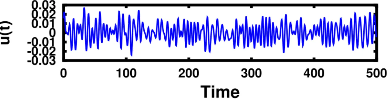
[44–49] for details. For T = 500, we obtain the control presented in Figure 1. The quality of the control, i.e. the quantity |⟨ψ(T),ψ(0)⟩|∥ψ(0)∥ is over 99% for all perturbations αk, k = 1, 2, 3. We also tested different pairs of initial and target states (ψ0, ψT) and in all cases high quality controls were found.
5. Extensions to an infinite set of perturbations We investigate in this section the circumstance when
K (the number of perturbations) is infinite. The
control-lability of a system consisting of an infinite collection of finite-dimensional systems has been analyzed for the situation of the Bloch equation (G = S O(3)) in [25– 27, 32]. To the best of our knowledge no general results are available for generic systems and values of N; more-over the counter-example in Theorem 4 in [27] warns that general results may be impossible to obtain.
We explore two questions: first we give an example that builds on the Maxwell-Bloch equation where a pos-itive controllability result is expected; next we give a procedure for the numerical identification of approxi-mate controls of a Bloch equation.
5.1. An example of perturbed Maxwell-Bloch equation
LetΩ a compact subset of R3 and recall the notation for the Pauli matrices:
σx= ( 0 1 1 0 ) , σy= ( 0 −i i 0 ) , σz= ( 1 0 0 −1 ) . (13) Consider the Maxwell-Bloch equation with two con-trols: idX(t, ω, α, β) dt = { ωσz+ [u(t) + α]σx+ [v(t)+ β]σy } X(t, ω, α, β), X(0, ω, α, β) = Id, (ω, α, β) ∈ Ω. (14)
Proposition 8. Let f = ( fx, fy, fz) :Ω → R3be a
con-tinuous function. Then, for anyη > 0 there exists a time Tη > 0 and two controls uη, vη ∈ L∞([0, Tη]) such that
for all (ω, α, β) ∈ Ω:
∥X(Tη, ω, α, β) − ei( fx(ω,α,β)σx+ fy(ω,α,β)σy+ fz(ω,α,β)σz)∥ ≤ η.
(15)
Proof. Although a rigorous proof of the controllability would require the tools in [32] and is beyond the scope of this work, we give below the arguments that indicate that this system is controllable. Consider the sequence of controls: start with u = −(π/2)δ0 (δ0 is the Dirac
-0.03
-0.02
-0.01
0
0.01
0.02
0.03
0
100
200
300
400
500
u(t)
Time
Figure 1: The control that drivesψ0toψT(cf. equation (10)) irrespective of the perturbationαk∈ {−0.1, 0, 0.1}. The quality of the control is over 99% for any perturbation. However the trajectoriesψ(t) corresponding to u(t) − 0.1, u(t) and u(t) + 0.1 are all different.
mass at the origin), followed by free evolution during a unit of time and then u= +(π/2)δ1. That is, choose u= −(π/2)δ0+ (π/2)δ1, v= 0. This results in the evolution
e−i(π/2)σxe−i(ωσz+ασx+βσy)ei(π/2)σx = e−i(−ωσz+ασx−βσy).
(16) Thus the propagator associated with−ωσz+ ασx− βσy can be synthesized. A similar computation (now using the control v) allows to construct−ωσz− ασx+ βσy. Using now infinitesimal times and the formula eU+V = limn→∞
(
eU/neV/n)n, we have thus at our disposal all propagators e±iωσz, e±iασx, e±iβσy. Recall that we also
have e±iσx, e±iσy.
From now on, the argument is similar to that in [27]: the formula lim n→∞ { e−χ/ne−ψ/neχ/neψ/n}n 2 = e[χ,ψ], (17) allows to use commutators of, for instance, ±iωσz and±iσxwhich produce±iωσyand then commutators ±iωσz and ±iωσy, which produce ±iω2σx; all other polynomials ofω can be obtained as multiplicative fac-tors in front of ωz. Similar arguments allow to fur-ther obtain all possible polynomials of three variables ω, α, β. Therefore we obtain approximate controllabil-ity of the system to any (smooth) target with L∞ con-trols.
Remark 4. 1. The result extends obviously to the Bloch equation (set on S O(3), see next section). 2. Not all situations have favorable outcomes. For in-stance, using same arguments as in Remark page 030302-2 of [26], it is possible to show that for the controlled Hamiltonianσz+ ασy+ u(t)σxthe un-known perturbationα ∈]α∗, α∗[ cannot always be compensated. Indeed, the attainable propagators
are of the form
exp{i f1(α2)(σy−ασz)+i f2(α2)(σz+ασy)+i f3(α2)σx} (18) where f1, f2 and f3 are arbitrary functions. Thus when for instanceΩ is symmetric with respect to α the functions f1, f2, f3are odd functions which is a restriction for controllability.
5.2. Convergence of the controls for a discrete set of perturbations
We investigate here a numerical algorithm to find the control when the set of perturbations can be a whole (possibly unbounded) closed interval Iα ⊂ R. Suppose
A, B ∈ g are such that LA,B = g and let us denote by
X(t, α, u) the solution of dX(t)dt = (A + (u(t) + α)B)X at
time t starting from X(0)= Id.
Consider also a continuous cost function to be mini-mized F : Iα× G → R+and to fix notations suppose that for any α ∈ Iα there exists some Zα ∈ G with
F(α, Zα) = 0. One interesting example of such func-tion is the distance F(α, Z) = ∥Z − Y(α)∥ to some pre-defined target Y(α) continuous with respect to α ∈ Iα. Of course Y can be in particular constant with respect to α. Consider a sequence of divisions Tℓ ⊂ Iα : αℓ
1 < αℓ1 < ... < αℓKℓ of the interval Iα such that
|Tℓ| := maxj=2,Kℓ|αℓj− αℓj−1| tends to 0 when ℓ tends to ∞. Fix also a tolerance η ≥ 0. Using the results of the previous sections there exists a time Tℓand a control uℓ such that F(αℓj, X(Tℓ, αℓj, uℓ))≤ η for all j = 1, ..., Kℓ. In this section, we give a sufficient result that ensures the existence of a control u that minimizes the cost F for the whole interval of perturbations Iαup to the toleranceη. Proposition 9. Suppose that the sequence Tℓis not con-verging to infinity and ∥uℓ∥Lr([0,T
ℓ]) are bounded by a
common constant for some 1 < r < ∞. Then there
exists T > 0 and u ∈ Lr([0, T]) (independent of α) such
that F(α, X(T, α, u)) ≤ η, for all α ∈ Iα.
Proof. Since Tℓ does not converge to∞ it has a sub-sequence converging to some T ∈ R. Denote again by Tℓthis subsequence; we can moreover consider that all Tℓ are either greater or smaller than T , let us say
Tℓ ≤ T for all ℓ. Extend the domain of definition of uℓ
on [0, T] with uℓ = 0 on [Tℓ, T]; this will not change its
Lr norm. Up to extracting another subsequence, there exists u ∈ Lr([0, T]) such that uℓ converges weakly in
L1([0, T]) to u. Let us prove that u satisfies the required conditions. Fixα ∈ Iα. Since|Tℓ| → 0, there exists a sequenceαℓk ℓsuch thatα ℓ kℓ → α when ℓ → ∞. We write: ∥X(Tℓ, αℓkℓ, uℓ)− X(T, α, u)∥ ≤ ∥X(Tℓ, αℓkℓ, uℓ)− e (T−Tℓ)AX(T ℓ, αℓkℓ, uℓ)∥ +∥e(T−Tℓ)AX(T ℓ, αℓkℓ, uℓ)− X(T, α, u)∥. (19) The term ∥X(Tℓ, αℓk ℓ, uℓ) − e (T−Tℓ)AX(T ℓ, αℓkℓ, uℓ)∥ is bounded by C∥Id − e(T−Tℓ)A∥ for some constant C > 0 and thus converges to 0. The last term can be written as:
∥e(T−Tℓ)AX(T ℓ, αℓkℓ, uℓ)− X(T, α, u)∥ = ∥e(T−Tℓ)AX(T ℓ, 0, αℓkℓ+ uℓ)− X(T, 0, α + u)∥ = ∥X(T, 0, αℓ kℓ+ uℓ+ 1[Tℓ,T]· (−αℓkℓ)) −X(T, 0, α + u)∥. (20)
Since Tℓ → T, it follows that αℓk
ℓ + uℓ+ 1[Tℓ,T]· (−α
ℓ kℓ) converges weakly in L1([0, T]) to α + u. From Theorem 3.6 of [50] (see also the Aubin-Lions lemma [51]), the weak convergence ofαℓk
ℓ+ uℓ+ 1[Tℓ,T]· (−α
ℓ
kℓ) toα + u ensures that limℓ→∞X(T, 0, αℓk
ℓ+ uℓ+ 1[Tℓ,T]· (−α
ℓ kℓ))=
X(T, 0, α + u). Combining all estimations, we obtain
limℓ→∞X(Tℓ, αℓk ℓ, uℓ)= X(T, α, u) thus F(α, X(T, α, u)) = lim ℓ→∞F(α ℓ kℓ, X(Tℓ, αℓkℓ, uℓ))≤ η, (21) and the conclusion follows.
Remark 5. The Proposition is not a controllability re-sult but can be used numerically to find the control when controllability holds true.
In particular the situationη = 0 corresponds to exact controllability; however the results in [32] show that ap-proximate controllability is more likely to hold and the controls will be in L∞loc, thus in all Lr([0, t]).
As a numerical illustration we consider the Bloch equation (which is a perturbation of the system in [32] forω = ω0) : d dt MMxy Mz = u(t)0+ α −(u(t) + α)0 −ω00 0 ω0 0 MMxy Mz , MMyx(0)(0) Mz(0) = M0,
where u(t) is the control. The system can be put into the framework of Proposition 9 by considering G= S O(3),
A= ω0 00 00 −10 0 1 0 , B = 01 −1 00 0 0 0 0 .
Let Mf be some target state. The goal to steer
M0 to Mf at time T can be rephrased as minimizing, with respect to u, F(α, X(T, α, u)) where F(α, Z) = ∥ZM0− Mf∥. The tolerance η is set to 5%. We take
M0 = (1, 0, 0)T and Mf = (0, 0, 1)T. The perturbation α takes all values in the interval Iα= [−αmax, αmax]; the divisionsTℓuse a Tchebytchev-type grid containing the points αℓk = αmaxcos(kπ/ℓ) with k = 0, · · · , Kℓ = ℓ. We consider the values of the parameters ω0 = 50,
T = 1000, αmax = 0.5 For the numerical resolution of the evolution equation in X(t, α, u) we use a Crank-Nicholson time-discretization scheme, with 103 time steps in [0, T]. To compute the optimal controls uℓ we apply again the monotonic procedure, see Section 4.
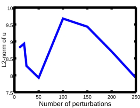
In order to check the assumptions of Proposition 9 we set r = 2 and verify that the ∥uℓ∥L2remain bounded
when ℓ increases. The norms ∥uℓ∥L2 are presented in
Figure 2 and are uniformly bounded with respect to ℓ. The quality of these controls is evaluated with
100 150 200 250 7.5 8 0 50 8.5 9 9.5 10 Number of perturbations L2-norm of u
Figure 2: Norms of∥uℓ∥L2forℓ = 5, 10, 25, 50, 100, 150, 200, 250.
F(α, X(T, α, uℓ)), which is in all cases lower thanη. In Figure 3, F(α, X(T, α, uℓ)) is plotted as a function ofα for the control field u250. We observe a very accurate control in the whole intervalα ∈ Iα(but the quality de-cays outside this interval).
6. Conclusion and perspectives
Necessary and sufficient conditions have been de-rived for the ensemble controllability of a finite collec-tion of bilinear systems on a connected, compact, sim-ple Lie group. The result was applied to the case where
0 0.5 1 0 0.05 0.1 -1 -0.5 0.15
Values of the perturbation
F
Figure 3: Values of F(α, X(T, α, uℓ)) forα ∈ [−1, 1]. The optimal control u250is applied. As expected the quality is within the tolerance
η in the interval Iαbut not outside it.
the control is submitted to a finite collection of constant or partially constant perturbations. The result extends to ensemble controllability and generalizes several works from the literature. Additional arguments have been presented when the number of possible perturbations is infinite.
This work studied the controllability for possibly large final times. A related question is whether small time local controllability (called STLC) is also true. A further question is whether the result extends to more general, time dependent, perturbations.
Acknowledgments
MB acknowledges support from the “Institut
Fran¸cais de Tunisie” (IFT). JS & GT acknowledge
support from the Agence Nationale de la Recherche (ANR), Projet Blanc EMAQS number ANR-2011-BS01-017-01. The authors thank C. Lefter (”Al. I. Cuza University” Ias¸i, Romania) for helpful discussions concerning this work and for proposing the model in Section 3.3.
References
[1] E.-D. Sontag, Mathematical control theory: deterministic finite dimensional systems, 2nd Edition, Springer, 1998.
[2] H.-K. Khalil, Nonlinear systems, Macmillan, 1996.
[3] H. Nijmeiher, A. van der Schaft, Nonlinear dynamical control systems, Springer, 1990.
[4] F. S. Leite, P.-E. Crouch, Controllability on classical Lie groups, Mathematics of Control, Signals, and Systems 1 (1988) 31–42. [5] V. Ramakrishna, M. Salapaka, M. Dahleh, H. Rabitz, A. Peirce,
Controllability of molecular-systems, Physical Review A 51 (1995) 960–966.
[6] D. D’Alessandro, Small time controllability of systems on com-pact Lie groups and spin angular momentum, J. Math. Phys. 42 (9) (2001) 4488–4496.
[7] F. Albertini, D. D’Alessandro, Notions of controllability for quantum mechanical systems, in: 40th IEEE Conference on De-cision and Control, Vol. 2, Orlando, FL, 2001, pp. 1589–1594. [8] C. Altafini, Controllability of quantum mechanical systems by
root space decomposition of su(n), Journal of Mathematical Physics 43 (5) (2002) 2051–2062.
[9] G. Turinici, H. Rabitz, Wavefunction controllability in quantum systems, Journal of Physics A: Mathematical and Theoretical 36 (2003) 2565–2576.
[10] S. Rice, M. Zhao, Optical control of quantum dynamics, Wiley, 2000.
[11] G. Huang, T. Tarn, J. Clark, On the controllability of quantum mechanical systems, J. Math. Phys. 24 (1983) 2608–2618. [12] R. Judson, K. Lehmann, H. Rabitz, W.-S. Warren, Optimal
design of external fields for controlling molecular motion-application to rotation, J. Molec. Structure 223 (1990) 425–456. [13] G. Turinici, On the controllability of bilinear quantum systems, in: M. Defranceschi, C. L. Bris (Eds.), Mathematical models and methods for ab initio Quantum Chemistry, Lecture Notes in Chemistry vol. 74, Springer, 2000, pp. 75–92.
[14] S.-G. Schirmer, H. Fu, A.-I. Solomon, Complete controllability of quantum systems, Phys. Rev. A 63 (2001) 063410. [15] G. Turinici, H. Rabitz, Quantum Wave Function Controllability,
Chemical Physics 267 (1-3) (2001) 1–9.
[16] M.-D. Girardeau, M. Ina, S.-G. Schirmer, T. Gulsrud, Kinemat-ical bounds on evolution and optimization of mixed quantum states, Phys. Rev. A 55 (1997) R1565–R1568.
[17] K. Beauchard, Local controllability of a 1-D Schr¨odinger equa-tion, Journal de Math´ematiques Pures et Appliqu´ees 84 (7) (2005) 851–956. doi:{10.1016/j.matpur.2005.02.005}. [18] K. Beauchard, C. Laurent, Local controllability of 1D linear and nonlinear Schr¨odinger equations with bilinear control, Journal de Math´ematiques Pures et Appliqu´ees 94 (5) (2010) 520–554. doi:{10.1016/j.matpur.2010.04.001}.
[19] M.-D. Girardeau, S.-G. Schirmer, J.-V. Leahy, R.-M. Koch, Kinematical bounds on optimization of observables for quantum states, Phys. Rev. A 58 (1998) 2684–2689.
[20] G. Turinici, V. Ramakrishna, B. Li, H. Rabitz, Optimal Discrim-ination of Multiple Quantum Systems: Controllability Analysis, J. Phys. A: Mathematical and General 37 (1) (2003) 273–282. [21] B. Li, G. Turinici, V. Ramakhrishna, H. Rabitz, Optimal
Dy-namic Discrimination of Similar Molecules Through Quantum Learning Control, Journal of Physical Chemistry B 106 (33) (2002) 8125–8131.
[22] G. Turinici, H. Rabitz, Optimally controlling the internal dy-namics of a randomly oriented ensemble of molecules, Phys. Rev. A 70 (6) (2004) 063412. doi:10.1103/PhysRevA.70. 063412.
[23] H. Rabitz, G. Turinici, Controlling quantum dynamics regard-less of laser beam spatial profile and molecular orientation, Physical review A: Atomic, Molecular and Optical Physics 75 (4) (2007) 043409.
[24] S.-G. Schirmer, I.-C. Pullen, A.-I. Solomon, Controllability of multi-partite quantum systems and selective excitation of quan-tum dots, Journal of Optics B 7 (2005) S293–S299.
[25] J.-S. Li, N. Khaneja, Ensemble controllability of the Bloch equations, in: 45th IEEE Conference on Decision and Control, San Diego, CA, USA, 2006, pp. 13–15.
[26] J.-S. Li, N. Khaneja, Control of inhomogeneous quantum en-sembles, Phys. Rev. A 73 (2006) 030302.
[27] J.-S. Li, N. Khaneja, Ensemble control of Bloch equations, IEEE Trans. Automat. Control 54 (3) (2009) 528–536. doi: 10.1109/TAC.2009.2012983.
URL http://dx.doi.org/10.1109/TAC.2009.2012983 [28] D. Sugny, A. Keller, O. Atabek, D. Daems, C. M. Dion,
S. Guerin, H.-R. Jauslin, Control of mixed-state quantum sys-tems by a train of short pulses, Physical Review A (Atomic, Molecular, and Optical Physics) 72 (3) (2005) 032704. [29] T.-J. Tarn, J. Clark, D. Lucarelli, Controllability of quantum
me-chanical systems with continuous spectra, in: Decision and Con-trol, 2000. Proceedings of the 39th IEEE Conference on, Vol. 1, 2000, pp. 943–948 vol.1. doi:10.1109/CDC.2000.912894. [30] C. Altafini, Controllability and simultaneous controllability of
isospectral bilinear control systems on complex flag manifolds, Systems & Control Letters 58 (2009) 213–216.
[31] K. Moore, H. Rabitz, Manipulating molecules, Nature Chem-istry 4 (2012) 72–73.
[32] K. Beauchard, J.-M. Coron, P. Rouchon, Controllability issues for continuous-spectrum systems and ensemble controllability of Bloch equations, Comm. Math. Phys. 296 (2) (2010) 525– 557. doi:10.1007/s00220-010-1008-9.
URL http://dx.doi.org/10.1007/s00220-010-1008-9 [33] K. Khodjasteh, L. Viola, Dynamical quantum error correction
of unitary operations with bounded controls, Phys. Rev. A 80 (2009) 032314. doi:10.1103/PhysRevA.80.032314. URL http://link.aps.org/doi/10.1103/PhysRevA. 80.032314
[34] K. Khodjasteh, L. Viola, Dynamically error-corrected gates for universal quantum computation, Phys. Rev. Lett. 102 (2009) 080501. doi:10.1103/PhysRevLett.102.080501. URL http://link.aps.org/doi/10.1103/ PhysRevLett.102.080501
[35] A. M. Souza, G. A. Alvarez,´ D. Suter, Experimen-tal protection of quantum gates against decoherence and control errors, Phys. Rev. A 86 (2012) 050301. doi:10.1103/PhysRevA.86.050301.
URL http://link.aps.org/doi/10.1103/PhysRevA. 86.050301
[36] D. Hocker, C. Brif, M. D. Grace, A. Donovan, T.-S. Ho, K. W. Moore Tibbetts, R. Wu, H. Rabitz, Characterization of control noise effects in optimal quantum unitary dynamics, ArXiv e-printsVersion 1. arXiv:1405.5950.
[37] I. R. Sola, H. Rabitz, The influence of laser field noise on controlled quantum dynamics, The Jour-nal of Chemical Physics 120 (19) (2004) 9009–9016. doi:http://dx.doi.org/10.1063/1.1691803.
URL http://scitation.aip.org/content/aip/ journal/jcp/120/19/10.1063/1.1691803
[38] S. Helgason, Differential geometry, Lie groups, and symmetric spaces, Vol. 34 of Graduate Studies in Mathematics, American Mathematical Society, Providence, RI, 2001, corrected reprint of the 1978 original.
[39] W. A. de Graaf, Lie algebras: theory and algo-rithms, Vol. 56 of North-Holland Mathematical Li-brary, North-Holland Publishing Co., Amsterdam, 2000. doi:10.1016/S0924-6509(00)80040-9.
URL http://dx.doi.org/10.1016/S0924-6509(00) 80040-9
[40] V. Jurdjevic, H. J. Sussmann, Control systems on Lie groups, J. Differ. Equations 12 (1972) 313–329.
[41] V. S. Varadarajan, Lie groups, Lie algebras, and their represen-tations, Vol. 102 of Graduate Texts in Mathematics, Springer-Verlag, New York, 1984, reprint of the 1974 edition. doi: 10.1007/978-1-4612-1126-6.
URL http://dx.doi.org/10.1007/978-1-4612-1126-6 [42] S. H. Tersigni, P. Gaspard, S. A. Rice, On using shaped light pulses to control the selectivity of product formation in a chemical reaction: An application to a multiple level system, The Journal of Chemical Physics 93 (3) (1990) 1670–1680. doi:http://dx.doi.org/10.1063/1.459680.
URL http://scitation.aip.org/content/aip/ journal/jcp/93/3/10.1063/1.459680
[43] Online controllability calculator.
URL https://www.ceremade.dauphine.fr/~turinici/ index.php/fr/recherche/calculator.html
[44] M. Belhadj, J. Salomon, G. Turinici, A stable toolkit method in quantum control, Journal of Physics A: Mathematical and The-oretical 41 (36) (2008) 362001–362011.
[45] D. Tannor, V. Kazakov, V. Orlov, Control of photochemical branching: Novel procedures for finding optimal pulses and global upper bounds, in: Time Dependent Quantum Molecu-lar Dynamics ed J Broeckhove and L Lathouwers, New York: Plenum, 1992, pp. 347–360.
[46] W. Zhu, H. Rabitz, A rapid monotonically convergent itera-tion algorithm for quantum optimal control over the expectaitera-tion value of a positive definite operator, J. Chem. Phys. 109 (1998) 385–391.
[47] S. G. Schirmer, M. D. Girardeau, J. V. Leahy, Efficient algorithm for optimal control of mixed-state quantum systems, Phys. Rev. A 61 (1999) 012101. doi:10.1103/PhysRevA.61.012101. [48] L. Baudouin, J. Salomon, Constructive solution of a bilinear
optimal control problem for a Schr¨odinger equation, Systems & Control Letters 57 (6) (2008) 453–464. doi:{10.1016/j. sysconle.2007.11.002}.
[49] Y. Maday, G. Turinici, New formulations of monotonically con-vergent quantum control algorithms, J. Chem. Phys. 118 (2003) 8191–8196.
[50] J. Ball, J. Marsden, M. Slemrod, Controllability for distributed bilinear systems, SIAM Journal on Control and Optimization 20 (4) (1982) 575–597. arXiv:http://dx.doi.org/10. 1137/0320042, doi:10.1137/0320042.
URL http://dx.doi.org/10.1137/0320042
[51] J.-P. Aubin, Un th´eor`eme de compacit´e, C. R. Acad. Sci. Paris 256 (1963) 5042–5044.
![Figure 3: Values of F( α, X(T , α, u ℓ )) for α ∈ [ − 1 , 1]. The optimal control u 250 is applied](https://thumb-eu.123doks.com/thumbv2/123doknet/14278414.491322/10.892.105.377.169.367/figure-values-f-α-ℓ-optimal-control-applied.webp)
