Scaling laws for the bifurcation-escape rate in a nanomechanical resonator

HAL Id: hal-01064458

https://hal.archives-ouvertes.fr/hal-01064458v2

Submitted on 23 Nov 2015

HAL is a multi-disciplinary open access

archive for the deposit and dissemination of

sci-entific research documents, whether they are

pub-lished or not. The documents may come from

teaching and research institutions in France or

abroad, or from public or private research centers.

L’archive ouverte pluridisciplinaire HAL, est

destinée au dépôt et à la diffusion de documents

scientifiques de niveau recherche, publiés ou non,

émanant des établissements d’enseignement et de

recherche français ou étrangers, des laboratoires

publics ou privés.

Distributed under a Creative Commons Attribution - ShareAlike| 4.0 International

License

Scaling laws for the bifurcation-escape rate in a

nanomechanical resonator

Martial Defoort, Vadim Puller, Olivier Bourgeois, Fabio Pistolesi, Eddy Collin

To cite this version:

Martial Defoort, Vadim Puller, Olivier Bourgeois, Fabio Pistolesi, Eddy Collin. Scaling laws for the

bifurcation-escape rate in a nanomechanical resonator. Physical Review E : Statistical, Nonlinear,

and Soft Matter Physics, American Physical Society, 2015, 92 (5), pp.050903(R).

�10.1103/Phys-RevE.92.050903�. �hal-01064458v2�

M. Defoort,1 _{V. Puller,}2 _{O. Bourgeois,}1 _{F. Pistolesi,}2 _{and E. Collin}1 1

Universit´e Grenoble Alpes, CNRS Institut N ´EEL, BP 166, 38042 Grenoble Cedex 9, France

2

Univ. Bordeaux, LOMA, UMR 5798, F-33400 Talence, France CNRS, LOMA, UMR 5798, F-33400 Talence, France

We report on experimental and theoretical studies of the fluctuation-induced escape time from a metastable state of a nanomechanical Duffing resonator in cryogenic environment. By tuning in situ the non-linear coefficient γ we could explore a wide range of the parameter space around the bifurcation point, where the metastable state becomes unstable. We measured in a relaxation process the distribution of the escape times. We have been able to verify its exponential distribution and extract the escape rate Γ. We investigated the scaling of Γ with respect to the distance to the bifurcation point and γ, finding an unprecedented quantitative agreement with the theoretical description of the stochastic problem. Simple power scaling laws turn out to hold in a large region of the parameter’s space, as anticipated by recent theoretical predictions. These unique findings, implemented in a model dynamical system, are relevant to all systems experiencing under-damped saddle-node bifurcation.

PACS numbers: 85.85.+j, 05.40.-a, 05.10.Gg, 05.70.Ln

Transition from a metastable to a stable state is a phenomenon of ubiquitous interest in science: in ther-mal equilibrium it is the essence of the activation law in chemistry [1, 2], it underlies nucleation in phase transi-tions, magnetization reversal in molecular magnets [3], biological switches in cells behavior [4] or RNA dynam-ics [5], transitions of Josephson junctions [6] or fluc-tuations in SQUIDs [7], the list being obviously non-exhaustive. More recently the study of escape statistics has been possible also for out-of-equilibrium dynamical systems like Penning traps [8], Josephson junctions [9], and nano-electromechanical systems [10–14]: the state-switching effect is extensively used in bifurcation ampli-fiers, with for instance state-of-the-art quantum bit read-out schemes [15]. In most of these cases the escape time distribution is exponential and the rate Γ characterizes completely the phenomenon. Analytical solutions [16] of the dynamical equations show that its value depends

ex-ponentially on a parameter D−1_{, that coincides with the}

(inverse of the) temperature for equilibrium systems and more generally is related to the power spectrum of the relevant fluctuations. One can then write:

Γ = Γ0exp(−Ea/D), (1)

where the prefactor Γ0is assumed to depend very weakly

on D, and Ea in analogy with a potential system can

be called activation energy: it parametrizes the distance to the unstable point. For out-of-equilibrium systems a central theoretical result is the paper by Dykman and

Krivoglaz [17], that found an explicit expression for Ea

and Γ0 for a generic dynamical system close to the

bi-furcation point, where the line of metastable states joins the line of unstable ones. It predicts universal power

laws dependence of Ea and Γ0 on the distance from the

bifurcation point in terms of |ω − ωb|, where ω is the

driving frequency of the dynamical system and ωb is its

bifurcation value.

Direct experimental measurement of the escape time

and study of the dependence of Ea and Γ0 over a wide

range of a system’s parameters is not a trivial task, since the exponential dependence of the escape time makes it either too long or too short for a reasonable observation protocol. For dynamical systems the resonating period fixes a lower bound on the time. Nano-mechanical res-onators with resonance frequency in the MHz range are thus a prominent choice to investigate the bifurcation in-stability of Duffing oscillators: they are high frequency dynamical systems with a high quality factor for which the distance to the bifurcation point can be directly con-trolled.

In the analysis of switching and reaction rates, three problems can thus be distinguished: obtaining the

expo-nent Ea, the prefactor Γ0, and their respective scalings

for systems away from thermal equilibrium. The expo-nent has been the first subject of interest, with the early work of Arrhenius [1]. The prefactor has then been ad-dressed by Kramers later on [2], while finally the scaling of both for dynamical systems has been derived by Dyk-man [17]. It is actually in micro and nano-mechanical systems that a measurement of the power law

depen-dence of Ea with respect to the distance from the

bi-furcation point has been performed, giving the predicted value within experimental error [10, 11]. Nevertheless, the activation energy has been claimed to match theory at best within a factor of 2 due to injected noise calibra-tion [10]. To our knowledge no attempts have been done to obtain a more quantitative verification of the predic-tions of Dykman and Krivoglaz [17], in particular for the

scaling law of the prefactor Γ0and the dependence to the

Duffing non-linear coefficient γ of both Γ0 and Ea.

An-swering the three above mentioned problems together is thus the aim of our work, using a unique nano-mechanical implementation of the bifurcation phenomenon.

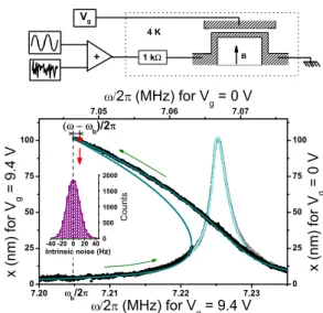
theoreti-2 7.05 7.06 7.07 0 25 50 75 100 7.20 7.21 7.22 7.23 0 25 50 75 100 x ( n m ) fo r V g = 0 V 2 (MHz) for V g = 0 V b )/2 V g x ( n m ) fo r V g = 9 .4 V 2 (MHz) for V g = 9.4 V -40-2002040 0 500 1000 1500 2000 Intrinsic noise (Hz) C o u n t s b /2 B + 1 k 4 K

FIG. 1: (Color online) Top panel: Schematic of the ex-perimental setup with the nano-resonator structure. Bottom panel: Linear and Duffing resonances (respectively grey and black points, with top-right and bottom-left axes). The lines show the fit. The nonlinear resonance is for Vg= 9.4 V, which shifts the resonance frequency and opens an hysteresis (thin green arrows highlight upward and downward sweeps). The relaxations occur at a detuning ω − ωb from the bifurcation frequency (red point and vertical arrow). Inset: Gaussian dis-tribution histogram of the measured intrinsic frequency fluc-tuations.

cal investigations of the dependence of Ea and Γ0on the

system parameters for a driven nano-mechanical oscilla-tor in the non-linear regime in presence of a controlled noise force. It is well known that for a sufficiently strong non-linear term the system admits for some values of the driving frequency a metastable solution. By measuring the escape rate for a wide range of parameters we could verify the validity of the power scaling laws predicted by

Dykman and Krivoglaz for both Ea and Γ0.

Remark-ably, we found that the scaling holds experimentally in a much larger region of the parameter space than the one for which the theory of Ref. [17] has been derived.

Con-cerning the Ea dependence on detuning, the possibility

of an extended region of scaling was discussed in Refs. [18, 19]. Performing the full numerical simulation of the stochastic problem adapted to our device parameters we found that experiment and theory are in excellent quan-titative agreement.

The experiment is performed on a unique goalpost

(depicted in top graph of Fig. 1) aluminum-coated

sili-con nano-electro-mechanical resonator. It sili-consists in two cantilever feet of length 3 µm linked by a paddle of length 7 µm, all about 250 nm wide and 150 nm thick for a total

mass m = 1.25 10−15 _{kg [20]. The experiment is}

per-formed at 4.2 K in cryogenic vacuum (pressure < 10−6

mbar). The motion is actuated and detected by means of the magnetomotive scheme [21], with a magnetic field

B < 1 T and a gate electrode is also capacitively cou-pled to the nanomechanical device (gap about 100 nm) [20]. The resonator admits large distortions (in the hun-dred nm range) to be attained while remaining intrinsi-cally extremely linear [22], while a well-controlled non-linearity can be generated by means of a DC gate

volt-age bias Vg [23]. This distinctive feature enables to tune

the global non-linearity of our device without changing the displacement amplitude. Using an adder we apply both a sinusoidal drive and a noise voltage from a voltage source generator. The resulting electric signal together with a 1 kOhm bias resistor is used to inject an AC cur-rent through the goalpost and generates both driving and controllable (zero average) noise forces on the resonator. More information on the calibration and experimental details can be found in Refs. [20, 22]. The resulting equa-tion of moequa-tion for the resonator displacement x reads:

¨

x + ∆ω ˙x + ω2

0x + γx3= fdcos(ωt) + fn(t) (2)

with ω0/2π=7.07 MHz the resonance frequency,

∆ω/2π=1.84 kHz the linewidth, and fd and fnthe drive

and noise forces divided by the mass of the resonator.

We fix the drive force so that mfd = 65 pN, leading to

a constant maximal displacement amplitude of 100 nm. As can be deduced from our characterizations [20], this amplitude is small enough to guarantee that nonlinear damping mechanisms such as discussed in Refs. [24, 25] are small (see comment in the discussion section). The noise force signal is filtered so that the force spectrum R

dteiωt_hf

n(t)fn(0)iω= 2D is constant over a bandwidth

of 1 MHz around 7 MHz. The Duffing coefficient γ

scales as V2

g and is for us negative [22]. At fixed driving

force, the system admits two amplitudes of oscillation

for sufficiently large |γ| as shown in Fig. 1 (bistability).

By fitting with the standard Duffing expressions [26] the

parameters ∆ω, ω0 and γ together with the bifurcation

frequency ωbcan be obtained with a good accuracy. The

experiment is then performed by sweeping ω from the

stable regime (ω > ω0) down to the edge of the hysteresis

at a given value of ω −ωbin the high amplitude state (see

Fig.1). The sweeping rate (a few Hz/s) is an important

parameter which should both guarantee adiabaticity of the sweep and high accuracy in the measurement [33]. Finally, the escape time from the metastable state is detected when the measured displacement amplitude

falls below an appropriate threshold value. Typically 103

escape events are recorded for each set of parameters. The experiment has been repeated for three different

values of the noise forces fn, three different detunings

ω − ωb (up to 5% of the hysteresis), and five different

values of Vg (and thus of γ), for a total of 45 escape

histograms. The resulting settings are summarized in

Fig.2.

For each data measurement, the experimental value

of ωb might slightly differ from the one obtained by the

initial fit. This problem is detected by sweeping rela-tively rapidly ω (tens of Hz/sec) through the

FIG. 2: (Color online) Bifurcation parameter space (normal-ized driving force versus Ω = 2|ω − ω0|/∆ω). The grey area is the NEMS bistability regime where the right edge is the transition from a high amplitude oscillation to a low one (the left edge is the opposite) and K is the spinode point where hysteresis starts to open. We show within the bistability the data points at different voltages Vg. Inset: typical low Vg re-laxation curve obtained with about 1000 rere-laxations, and fit with and without fluctuations on ωb.

each relaxation-time acquisition. A typical histogram of

the distribution of ωb is shown in the inset of Fig.1 for

Vg = 9.4 V. It has Gaussian form with a half-width σ

in the range of tens of Hz. This tiny spread (10−6 _to

10−5 _{of ω}

b) is due to low-frequency intrinsic fluctuations

of the resonating frequency, which actual origin is still under debate [27–29]. Even if extremely small, due to the high sensitivity of the bifurcation phenomenon the

fluctuations of ωb modify slightly the value of Γ at each

measurement, and we have to take this effect into ac-count. The escape exponential distribution has thus to

be averaged over these fluctuations. For |ω −ωb| ≫ σ one

can expand this dependence: Γ(ω−ωb−ǫ) = Γ+Γ′ǫ+. . . ,

where ǫ is the Gaussian-distributed shift of ωb. This gives

the following distribution for the escape times:

P (t) = Γe−Γt

Z _dǫ

σ√2πe

−ǫ2_/(2σ2_)−Γ′_ǫt

. (3)

Fitting it to the data with the method of Kolmogorov-Smirnov [30], to avoid losses of information due to his-togram binning, the two independent parameters of the

distribution, Γ and the product Γ′_{σ, can be obtained.}

A typical curve is shown in the inset of Fig. 2. Note

that this procedure does not need any hypothesis on the

explicit functional dependence of Γ on ωb. On the other

hand the procedure breaks down for too small detunings, and we thus need to drop the data for four values of the

detuning. We can then verify the validity of Eq. (1) for

the system at hand by plotting log Γ as a function of 1/D

(see Fig.3). The linear fit gives Eaand Γ0. The absolute

experimental definition of the noise level is difficult, and we introduce a calibration factor C (close to 1) between D and the nominal injected noise power. Note that it

simply amounts to multiply Ea by C, thus leaving the

0.0 0.5 1.0 10 -1 10 0 10 1 10 2 700 Hz 400 Hz 100 Hz Exponential Fit -1 s ) D -1 (N -2 /kg -2 Hz -1 )

FIG. 3: (Color online) Escape time as a function of D−1 _for Vg= 9.4 V at different detunings ω − ωbfrom the bifurcation point.

scaling dependence unmodified. The value of Γ0 is not

affected by this calibration either. More experimental details can be found in Ref. [31].

In order to extract the scaling dependence of Ea and

Γ0 on the detuning and the non-linear parameter γ it is

convenient to recall the predictions that can be obtained following Ref. [17]. Let us rescale the detuning by

defin-ing Ω = 2|ω − ω0|/∆ω with Ωb = 2|ωb− ω0|/∆ω. For

Ωb≫

√

3 (that holds for all the data of our experiment)

one obtains that Ωb≈ 3|γ|fd2/(4ω2∆ω2) with the

param-eters in Eq. (1) reading [34]:

Ea = 2f 2 d 3∆ω |Ω − Ωb|3/2 Ω5/2b , Γ0=∆ω 2 |Ω − Ωb|1/2Ω1/2b 2π . (4)

The basic assumptions to obtain these expressions are

that Ea/D ≫ 1 in order to keep the escape a rare event,

and to be able to reduce this two-dimensional problem (amplitude and phase) into a one-dimensional one. This second condition (much less appreciated in the literature) is only verified when the driving frequency ω is in a tiny

region close to the bifurcation point ωb and far from the

frequency for which the amplitude is maximum. In this region, one of the eigenvalues of the linearized dynamical equations of motion vanishes, which induces a slow mo-tion in the direcmo-tion of the relative eigenvector. On the other hand when ω is such that the amplitude is max-imal, the two eigenvalues coincide, inducing fully two-dimensional fluctuations. Thus beyond this point the

approximation used to obtain Eq. (4) breaks down. This

condition reads 4Ωb|Ω − Ωb| ≪ 1.

In the experiment we performed this quantity ranged uniformly between 0.13 to 71, thus a part of the data where well outside the range of the expected validity of

Eq. (4), enabling to investigate the behavior of Γ in a

region where no present analytical prediction exists. As

de-4 5x10 -4 5x10 -3 10 1 10 2 10 3 5 15 10 -2 10 -1 10 0 E a ( N 2 / k g 2 H z ) b 5/3 b b E a b | -3 / 2 0.1 1 10 10 1 10 2 10 3 10 4 3 10 10 1 10 2 0 ( H z) | b | b b 0 | b | -1 / 2

FIG. 4: (Color online) Scaling plots for Ea (left) and Γ0 (right) with respect to detuning. The full circles indicate the experimental points, the open (blue) triangles the prediction of the full numerical simulation, the (red) full lines the linear fit to the data, and the dashed (blue) lines the prediction of Eq. (4). Insets: scaling with the non-linear parameter Ωb.

pend only on the detuning and the non linear coefficient

(through Ωb), the other parameters being the same for all

data points. To test the validity of Dykman-Krivoglaz ex-pressions, we produce a scaling plot, where the logarithm

of Ea and Γ0 are plotted as a function of |Ω − Ωb|/Ω5/3b

and |Ω − Ωb|Ωb(see Fig.4). A remarkable scaling is then

observed in all the experimental range, with a fitted slope as a function of the detuning of 1.53±0.04 and 0.55±0.2,

for Ea and Γ0 respectively. This matches the analytic

predictions by Dykman and Krivoglaz, and we use this good agreement to define the noise source calibration

fac-tor C: scaling D by C the prediction of Eq. (4) coincides

with the fitted value for Ea (dashed line in Fig. 4 left

panel). The dependence on the non-linear parameter Ωb

could also be tested for both quantities. It is shown in

the insets of Fig.4and gives fitted slopes of −2.43 ± 0.05

and 0.6 ± 0.1, again in excellent agreement with Eq. (4).

To better understand this remarkable scaling in such a large parameter region we solved numerically the stochas-tic problem. This can be done by introducing the

com-plex slow amplitude z(t) defined as x(t) = z(t)eiωt₊

z(t)∗_e−iωt _{and then convert the Langevin Eq. (2) to a}

Fokker-Planck equation ∂τP = LP for the

probabil-ity densprobabil-ity P (u, v, τ ) of the real and imaginary part of

z = (3|γ|/∆ω)1/2_{(u + iv) as a function of the}

dimension-less time τ = t∆ω. The escape rate from a given domain

can be calculated by solving the equation L†_{τ (u, v) = −1}

with zero boundary condition at the border of the domain [16]. This gives the average time needed to reach the bor-der starting at (u, v). The equation reads explicitly:

[D(∂2u+ ∂2v) − fu∂u− fv∂v]τ = −1 , (5)

with D = 3|γ|D/(8ω3_{∆ω), f}

u= u + v(u2+ v2) − Ω, fv=

v−u(u2_+v2_)−Ω−F

d, and Fd= fd(3|γ|)1/2/[2(ω∆ω)3/2].

Eq. (5) can be solved numerically [32] to obtain the

av-erage escape time that coincides with the inverse of the

sought Poissonian rate. The numerical results for Eaand

Γ0 are shown in Fig.4in open (blue) triangles.

One can see that the exact (numerical) result has the same power law dependence as the analytical results (dashed line), even where the approximate theory is not supposed to hold. Quantitative agreement between

ex-periment and theory on Ea is obtained with C ≈ 1.3,

thus validating the experimental noise amplitude calibra-tion to within 15 % which is remarkable. Note that the simulation does not contain any other free parameter, which are all experimentally known to better than 5 %.

Concerning Γ0, we are not aware of previous attempts

to compare this quantity to the theoretical predictions. The agreement with the full theory is within a factor of about 3, which is remarkable given the logarithmic pre-cision on this parameter. We speculate that these dis-crepancies could arise from the actual algorithm used to

extract Γ0, or from more fundamental reasons like

ex-tra (non-Duffing) nonlinearities appearing in Eq. (2) (i.e.

non-linear damping, or non-cubic restoring force terms) [35].

In conclusion, we have investigated the escape dynam-ics close to the bifurcation point for a nanomechanical resonator in the Duffing non-linear regime measured at cryogenic temperatures. Using a single ideally tunable system, we have: (i) Measured the escape rate Γ as a function of the noise amplitude D, the detuning to the

bifurcation point ω − ωb, and the nonlinear parameter

γ. (ii) Extracted Ea and Γ0 as defined by Eq. (1). (iii)

Verified that the universal scaling of Ea and Γ0 initially

predicted for a tiny region around the bifurcation point holds actually in a region up to two orders of magnitude larger than the original one. (iv) Verified by solving nu-merically the exact problem, that the observation is in quantitative agreement with the behavior expected for a

driven Duffing oscillator. The scaling of Ea as a

[18, 19]. Due to the generality of the Duffing model, these results are of interest for a wide class of systems. Even beyond the fundamental interest in the scaling laws we point out that the device acts as a very sensitive am-plifier: it allows the detection of tiny variations of the resonator frequency. Understanding the frequency fluc-tuations in mechanical resonators is a current challenge of the field [27–29]. Mastering of the bifurcation escape technique by having a reliable theory and experimental

verification of the scaling of the rates is a crucial step towards the study of modifications induced by other phe-nomena.

We gratefully acknowledge discussions with M. Dyk-man, K. Hasselbach, E. Lhotel and A. Fefferman. We thank J. Minet and C. Guttin for help in setting up

the experiment. We acknowledge support from

MI-CROKELVIN, the EU FRP7 grant 228464 and of the

French ANR grant QNM n◦ _{0404 01.}

[1]S. Arrhenius, Z. Physik. Chem. 4, 226 (1889).

[2]H. A. Kramers,Physica 7, 284 (1940).

[3]M. A. Novak, R. Sessoli, A. Caneschi, and D. Gatteschi,

J. of Magn. and Magn. Mater. 146, 211 (1995).

[4]E. M. Ozbudak, M. Thattai, H. N. Lim, B. I. Shraiman, and A. van Oudenaarden,Nature 427, 737 (2004).

[5]E. A. Dethoff, J. Chugh, A. M. Mustoe, and H. M. Al-Hashimi, Nature 482, 322 (2012).

[6]E. Turlot, D. Esteve, C. Urbina, J. M. Marti-nis, M. H. Devoret, S. Linkwitz, and H. Grabert,

Phys. Rev. Lett. 62, 1788 (1989).

[7]J. Kurkijrvi,Phys. Rev. B 6, 832 (1972).

[8]L. J. Lapidus, D. Enzer, and G. Gabrielse,

Phys. Rev. Lett. 83, 899 (1999).

[9]I. Siddiqi, R. Vijay, F. Pierre, C. M. Wilson, M. Met-calfe, C. Rigetti, L. Frunzio, and M. H. Devoret,

Phys. Rev. Lett. 93, 207002 (2004).

[10] J. S. Aldridge and A. N. Cleland,

Phys. Rev. Lett. 94, 156403 (2005).

[11] C. Stambaugh and H. B. Chan,

Phys. Rev. B 73, 172302 (2006).

[12] H. B. Chan and C. Stambaugh,

Phys. Rev. Lett. 99, 060601 (2007).

[13] H. B. Chan, M. I. Dykman, and C. Stambaugh,

Phys. Rev. Lett. 100, 130602 (2008).

[14] Q. P. Unterreithmeier, T. Faust, and J. P. Kotthaus,

Phys. Rev. B 81, 241405 (2010).

[15] N. Boulant, G. Ithier, P. Meeson, F. Nguyen, D. Vion, D. Esteve, I. Siddiqi, R. Vijay, C. Rigetti, F. Pierre, and M. Devoret, Phys. Rev. B 76, 014525 (2007).

[16] P. H¨anggi, P. Talkner, and M. Borkovec,

Rev. Mod. Phys. 62, 251 (1990).

[17] M. I. Dykman and M. A. Krivoglaz, Sov. Phys. JETP , 60 (1979).

[18] M. Dykman, I. Schwartz, and M. Shapiro, Phys. Rev. E 72_{, 021102 (2005).}

[19] O. Kogan, arXiv:0805.0972v2 (2008).

[20] E. Collin, M. Defoort, K. Lulla, T. Moutonet, J.-S. Heron, O. Bourgeois, Y. M. Bunkov, and H. Godfrin,

Review of Scientific Instruments 83, 045005 (2012).

[21] A. Cleland and M. Roukes, Sensors and Actuators 72, 256 (1999).

[22] E. Collin, T. Moutonet, J.-S. Heron, O. Bour-geois, Y. M. Bunkov, and H. Godfrin,

J Low Temp Phys 162, 653 (2011).

[23] I. Kozinsky, H. W. C. Postma, I. Bargatin, and M. L. Roukes,Applied Physics Letters 88, 253101 (2006).

[24] S. Zaitsev, O. Shtempluck, E. Buks, and O. Gottlieb, Nonlinear Dynamics 67, 859 (2012).

[25] E. Collin, T. Moutonet, J.-S. Heron, O. Bourgeois, Y. M. Bunkov, and H. Godfrin, Phys. Rev. B 84, 054108 (2011).

[26] E. Collin, Y. M. Bunkov, and H. Godfrin,

Phys. Rev. B 82, 235416 (2010).

[27] K. Y. Fong, W. H. P. Pernice, and H. X. Tang,

Phys. Rev. B 85, 161410(R) (2012).

[28] Y. Zhang, J. Moser, J. G¨uttinger, A. Bachtold, and M. I. Dykman, Phys. Rev. Lett. 113, 255502 (2014).

[29] R. van Leeuwen, A. Castellanos-Gomez, G. Steele, H. van der Zant, and W. Venstra, Appl. Phys. Lett. 105_{, 041911 (2014).}

[30] W. Eadie, D. Drijard, F. James, M. Roos, and B. Sadoulet, Statistical Methods in Experimental Physics, edited by North-Holland (Amsterdam, 1971).

[31] M. Defoort, PhD thesis: Non-linear dynamics in nano-electromechanical systems at low temperature (CNRS et Universit´e Grenoble Alpes, unpublished, 2014).

[32] F. Pistolesi, Y. Blanter, and I. Martin,

Physical Review B 78, 085127 (2008).

[33] We can estimate adiabaticity using theoretical expres-sions from Ref. [24]. Eqs. (50), (53) and (57) give the shift in bifurcation frequency δerrinduced by finite sweep

rate. We obtain δerr= 2π 0.5 Hz at most with our

exper-imental parameters, which means that the error in the resonance position is less than 20 ppm of the Duffing fre-quency shift itself. At the same time, the critical slowing down time τsd can be estimated from Eq. (52). We

ob-tain τsdsmaller than 8 ms for all our settings, which shall

be compared to the smallest recorded bifurcation time of order 40 ms.

[34] These expressions are obtained following the method of Ref. [17]. Note that in our work the bifurcation is anal-ysed as a function of frequency detuning and nonlinear parameter (not applied force).

[35] We tried to quantify the impact of nonlinear damping and of gate coupling non-Duffing contributions on the dynam-ics equation. Using a quadratic fit to describe nonlinear damping [25, 26], one can estimate the p parameter of Ref. [24] to be at worst about 0.06. Following the cal-culation procedure of Ref. [17], the alteration of the en-ergy potential Eais then at worst about 20 %. From the

gate capacitance Taylor series coefficients of Ref. [20], we calculate that the ”effective” Duffing nonlinear parame-ter measured in a frequency-sweep experiment could be modified by about 4 % with respect to the value com-puted from the actual x3

restoring force term, which is small.