HAL Id: hal-00318087
https://hal.archives-ouvertes.fr/hal-00318087
Submitted on 23 Dec 2005
HAL is a multi-disciplinary open access
archive for the deposit and dissemination of
sci-entific research documents, whether they are
pub-lished or not. The documents may come from
teaching and research institutions in France or
abroad, or from public or private research centers.
L’archive ouverte pluridisciplinaire HAL, est
destinée au dépôt et à la diffusion de documents
scientifiques de niveau recherche, publiés ou non,
émanant des établissements d’enseignement et de
recherche français ou étrangers, des laboratoires
publics ou privés.
and temperature at mid-latitudes from SATI
observations
M. J. López-González, Elizandro Rodriguez, G. G. Shepherd, S. Sargoytchev,
M. G. Shepherd, V. M. Aushev, S. Brown, M. Garcia-Comas, R. H. Wiens
To cite this version:
M. J. López-González, Elizandro Rodriguez, G. G. Shepherd, S. Sargoytchev, M. G. Shepherd, et
al.. Tidal variations of O2 Atmospheric and OH(6-2) airglow and temperature at mid-latitudes from
SATI observations. Annales Geophysicae, European Geosciences Union, 2005, 23 (12), pp.3579-3590.
�hal-00318087�
Geophysicae
Tidal variations of O
2
Atmospheric and OH(6-2) airglow and
temperature at mid-latitudes from SATI observations
M. J. L´opez-Gonz´alez1, E. Rodr´ıguez1, G. G. Shepherd2, S. Sargoytchev2, M. G. Shepherd2, V. M. Aushev3, S. Brown2, M. Garc´ıa-Comas1, and R. H. Wiens4
1Instituto de Astrof´ısica de Andaluc´ıa, CSIC, P.O. Box 3004, E-18080 Granada, Spain
2Centre for Research in Earth and Space Science, York University, 4700 Keele St., Toronto, Ontario M3J 1P3, Canada 3Institute of Ionosphere, Ministry of Education and Science, Almaty, 480020, Kazakhstan
4Department of Physics, University of Asmara, Eritrea, N. E. Africa
Received: 16 September 2005 – Revised: 18 October 2005 – Accepted: 27 October 2005 – Published: 23 December 2005
Abstract. Airglow observations with a Spectral Airglow
Temperature Imager (SATI), installed at the Sierra Nevada Observatory (37.06◦N, 3.38◦W) at 2900-m height, have been used to investigate the presence of tidal variations at mid-latitudes in the mesosphere/lower thermosphere region. Diurnal variations of the column emission rate and vertically averaged temperature of the O2Atmospheric (0-1) band and
of the OH Meinel (6-2) band from 5 years (1998–2003) of observations have been analysed. From these observations a clear tidal variation of both emission rates and rotational temperatures is inferred. It is found that the amplitude of the daily variation for both emission rates and temperatures is greater from late autumn to spring than during summer. The amplitude decreases by more than a factor of two dur-ing summer and early autumn with respect to the amplitude in the winter-spring months. Although the tidal modulations are preferentially semidiurnal in both rotational temperatures and emission rates during the whole year, during early spring the tidal modulations seem to be more consistent with a di-urnal modulation in both rotational temperatures and emis-sion rates. Moreover, the OH emisemis-sion rate from late au-tumn to early winter has a pattern suggesting both diurnal and semidiurnal tidal modulations.
Keywords. Atmospheric composition and structure
(Air-glow and aurora; pressure density and temperature; instru-ments and techniques)
1 Introduction
Airglow emissions have been used to study the chemical and dynamical behaviour of the atmosphere in those regions Correspondence to: M. J. L´opez-Gonz´alez
where the emission takes place. Atmospheric tides are the global response of the atmosphere to the periodic forcing of solar heating. The influence of the atmospheric tides on the airglow emissions has been studied since 1970 (e.g. Wiens and Weill, 1973; Petitdidier and Teitelbaum, 1977; Takahashi et al., 1977). The tides present periodicities equal to the so-lar day and its harmonics, and propagate westward following the motion of the Sun (e.g. Chapman and Lindzen, 1970).
There is an enormous body of ground-based observations of the mesosphere and lower thermosphere by the global radar network (e.g. Jacobi et al., 1999; Pancheva et al., 2000, 2002; Riggin et al., 2003; Forbes et al., 2004; Manson et al., 2004; Portnyagin et al., 2004) that have been used to study the tidal behaviour of the atmospheric winds. Stud-ies of the influences of atmospheric tides on airglow emis-sion and temperature using long-term, ground-based obser-vations (e.g. Wiens and Weill, 1973; Petitdidier and Teitel-baum, 1977; Scheer and Reisin, 1990; Reisin and Scheer, 1996; Takahashi et al., 1998; Choi et al., 1998) and satellite airglow observations (Abreu and Yee, 1989; Burrage et al., 1994; Shepherd et al., 1995, 1998) have shown a large vari-ation in diurnal behaviour of the airglow emission rates as a function of the year and of the latitude.
Simultaneous satellite observations of emission rates, tem-peratures and winds performed with the High Resolution Doppler Imager (HRDI) and Wind Imaging Interferometer (WINDII), both on board the UARS satellite, have been used to study the tidal variations in airglow emission rates and winds (Burrage et al., 1994; Shepherd et al., 1995, 1998; Shepherd et al., 2004a).
Here, we analysed the tidal variation found from long-term, ground-based airglow observations at 37.06◦N lati-tude. These observations have been made by a Spectral Airglow Temperature Imager (SATI) instrument placed at the Sierra Nevada Observatory. This instrument is able to
measure the column emission rate and the vertically aver-aged rotational temperature of both the O2Atmospheric
(0-1) band, and the OH Meinel (6-2) band, using the technique of interference filter spectral imaging with a cooled CCD de-tector (Wiens et al., 1997). The data analysed cover a period from 1998 to 2003. Tidal variations of the temperature and airglow emission rates of the O2Atmospheric (0-1) band and
the OH Meinel (6-2) band are presented and compared with previous results. It is shown that the diurnal variation of the emission rates and temperatures has a seasonal dependence. The amplitudes of the variations observed during late autumn to spring are greater by more than a factor of two than those observed during the rest of the year.
2 Observations
SATI is installed at the Sierra Nevada Observatory (37.06◦N, 3.38◦W), Granada, Spain, at 2900-m height. It has been in
continuous operation since October 1998. SATI is a spatial and spectral imaging Fabry-Perot spectrometer in which the etalon is a narrow band interference filter and the detector is a CCD camera. The SATI instrumental concept and opti-cal configuration was originally developed as the Mesopause Oxygen Rotational Temperature Imager (MORTI) instru-ment (Wiens et al., 1991). The new adaptation as SATI is described in detail by Sargoytchev et al. (2004). The instru-ment uses two interference filters, one centred at 867.689 nm (in the spectral region of the O2Atmospheric (0-1) band) and
the second one centred at 836.813 nm (in the spectral region of the OH Meinel (6-2) band). Its field of view is an annu-lus of 30◦ average radius and 7.1◦ angular width, centered on the zenith. Thus, an annulus of average radius of 55 km and 16 km width at 95 km (or an average radius of 49 km and 14 km width at 85 km) is observed in the sky.
The images are disks where the polar angle dimension cor-responds to the azimuth of the ring of the sky observed, while the radial distribution of the images contains the spectral dis-tribution, from which the rotational temperature is inferred. The method of SATI image reduction and temperature and emission rate determination was described in detail by Wiens et al. (1991) for the O2Atmospheric system, and by
L´opez-Gonz´alez et al. (2004) for the OH(6-2) Meinel band. In this work the images obtained from SATI are analysed as a whole, obtaining an average of the rotational temperature and emission rate of the airglow band from the whole sky ring.
The seasonal variation in rotational temperatures and air-glow emission rates measured with the SATI instrument dur-ing the period of October 1998 to March 2002 have been analysed and presented by L´opez-Gonz´alez et al. (2004). In the current study new data from March 2002 to May 2003 have been added to the earlier data set and are analysed, in order to derive the tidal variations present in both rota-tional temperatures and emission rates. The OH tempera-tures deduced from the Q-branch have been corrected from
the error introduced by using Q-branch theoretical Einstein coefficients (see Pendleton and Taylor, 2002).
Table 1 shows the number of days and hours of observation used in the study, in each month from October 1998 to May 2003. Table 1 also shows the total number of days and hours per month. We have used all the data corresponding to good observing conditions, even data corresponding to short days of observations, with the aim of obtaining the largest amount of data.
There are months, such as January 1999, when only two short nights of data are available, and the nocturnal variation of this month covers only one-third of the night compared with January data of other years. However, although only one-third of the night was covered, a strong correlation ex-isted with the nocturnal variation during this one-third of the night and that obtained during the January nights of other years.
L´opez-Gonz´alez et al. (2004) have shown that rotational temperatures and emission rates have a marked short-term variability together with a clear seasonal variation. Tables 2 and 3 show the mean rotational temperatures (TO2 and TOH) and emission rates (EO2and EOH) for each month of the year due to the seasonal variation of these parameters found in SATI data. In Tables 2 and 3 are also listed other quanti-ties that will be discussed in the following section: the abso-lute amplitudes of the temperature and emission rate varia-tions (1TO2, 1TOH, 1EO2 and 1EOH), the relative temper-ature and emission rate amplitudes, (1TO2
TO2 , 1TOH TOH , 1EO2 EO2 and 1EOH
EOH ), the amplitudes and phases of the Krassovsky ratio (|η|,φ) and the vertical wavelengths (λz) for the propagation
of the tidal modulations found from both emissions.
Here our interest is to determine the tidal variations and the seasonal dependences of these tidal variations. First of all, we subtracted the annual and semiannual seasonal variations in the rotational temperature and emission rates of both OH and O2emissions (see Tables 2 and 3). Here we employ the
residual temperatures and emission rates after removing the seasonal dependences.
For the systematic organization of the data we average these residual rotational temperatures and emission rates from each night over 30-min intervals, centered on the hours and half hours. Thus, an averaged nighttime variation is ob-tained for each night of available data, for every night of the month. This reduces short-period variations but does not af-fect tidal components. By averaging the values obtained at the same local time over one month, we obtain the diurnal variation for each month of available observations in each year of SATI observations. A “mean” monthly diurnal vari-ation is then derived by averaging the monthly diurnal varia-tions over the 5-year period.
3 Results
The averaged diurnal variations, for each month, from 1998 to 2003, together with the “mean” diurnal variation, are
Table 1. Airglow observations.
1998 1999 2000 2001 2002 2003 Total
Month nights hours nights hours nights hours nights hours nights hours nights hours nights hours
January 2 7 6 23 5 27 12 90 25 151 February 17 94 13 150 3 20 16 109 8 69 57 373 March 15 93 14 122 19 119 11 62 59 396 April 9 69 9 58 11 63 29 193 May 5 36 12 80 12 67 29 183 June 5 34 8 36 21 84 38 154 July 15 81 4 17 5 24 23 85 47 207 August 5 20 18 105 6 30 22 103 51 258 September 12 67 12 85 19 100 43 252 October 22 174 6 36 16 112 18 90 11 43 73 455 November 23 172 9 88 18 98 50 358 December 11 86 11 89 6 26 19 91 47 292
Table 2. Summary of wave parameters from OH layer. Solutions obtained from amplitudes smaller than 3 K are listed in bold.
Month EOH(R) 1EOH(R) 1EEOH OH TOH(K) 1TOH(K) 1TTOH OH |η| φ(degree) λz(km) January 793 171.2 0.216 211 4.8 0.0228 9.5 −77.9 −14.3 February 692 178.3 0.258 208 6.5 0.0314 8.2 −70.7 −17.0 March 637 188.7 0.296 205 5.4 0.0265 11.2 −88.7 −11.8 April 652 160.9 0.247 199 2.6 0.0129 19.1 −158.9 −19.1 May 690 151.8 0.220 192 1.2 0.0060 36.7 +138.4 +5.4 June 686 101.0 0.147 186 − − − − − July 672 93.5 0.139 185 − − − − − August 572 106.7 0.187 191 0.8 0.0039 47.9 −142.9 −4.6 September 591 104.3 0.176 200 2.2 0.0110 16.0 +64.4 +9.1 October 694 94.4 0.136 209 1.6 0.0074 18.4 −115.4 −8.0 November 813 166.0 0.204 213 6.0 0.0282 7.2 −112.1 −19.7 December 862 142.7 0.165 214 5.2 0.0243 6.8 −99.5 −19.7
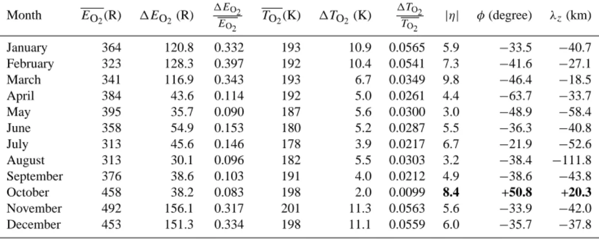
Table 3. Summary of wave parameters from O2layer. Solutions obtained from amplitudes smaller than 3 K are listed in bold.
Month EO2(R) 1EO2(R) 1EO2 EO2 TO2(K) 1TO2 (K) 1TO2 TO2 |η| φ(degree) λz(km) January 364 120.8 0.332 193 10.9 0.0565 5.9 −33.5 −40.7 February 323 128.3 0.397 192 10.4 0.0541 7.3 −41.6 −27.1 March 341 116.9 0.343 193 6.7 0.0349 9.8 −46.4 −18.5 April 384 43.6 0.114 192 5.0 0.0261 4.4 −63.7 −33.7 May 395 35.7 0.090 187 5.6 0.0300 3.0 −48.9 −58.4 June 358 54.9 0.153 180 5.2 0.0287 5.5 −36.3 −40.8 July 313 45.6 0.146 178 3.9 0.0217 6.7 −21.9 −52.6 August 313 30.1 0.096 182 5.5 0.0303 3.2 −38.4 −111.8 September 376 38.6 0.103 191 4.0 0.0212 4.9 −38.6 −43.8 October 458 38.2 0.083 198 2.0 0.0099 8.4 +50.8 +20.3 November 492 156.1 0.317 201 11.3 0.0563 5.6 −33.9 −42.0 December 453 151.3 0.334 198 11.1 0.0559 6.0 −35.7 −37.8
Fig. 1. Emission rates and rotational temperatures after removing seasonal annual and semiannual variations. Red circles: 1998. Green
triangles: 1999. Blue squares: 2000. Blue crosses: 2001. Pink asterisks: 2002. Yellow stars: 2003. Solid line: Mean monthly night variations.
plotted in Fig. 1. The results show that the diurnal pattern ob-tained for each month is very similar for the different years from 1998 to 2003, and so is the “mean” monthly diurnal variation averaged over all years. Thus, it is easy to see for all years, for example, that in January the O2emission rate
begins to decrease, creating minima at about four hours be-fore midnight, and then increases until maxima are formed about 2 or 3 h after midnight (even in January 1999, where less than 4 h of data are available, these data follow the same behaviour as the other January months). However, the OH emission rate begins to decrease, creating minimum values at midnight. On the other hand, O2 rotational temperature
(TO2) and OH rotational temperature (TOH) have a similar pattern of variation to that of the O2emission rate, although
the maximum values of the O2temperature are reached about
two hours earlier. Different patterns of diurnal variations are found for each month of the year. The presence of a modu-lation with a time period of 12 h is clearly seen in the winter months in both rotational temperatures and O2emission rates
(see Fig. 1).
The number of night hours of each month goes from around 7 h in June to about 12 h of night coverage in De-cember. Crary and Forbes (1983) showed that it is possible
to extract semidiurnal and diurnal tides using data of lim-ited temporal length, if these are closely spaced and aver-aged over several nights. Since we are working with data measured in exposure times of 2 min, averaged over the dif-ferent days of each month during 5 years, we can have some qualitative information about the relative significance of the tidal components, but this nocturnal coverage is insufficient for finding a unique mathematical solution of the different tidal components (see Wiens et al., 1995).
The amplitudes and phases for diurnal and/or semidiurnal modulations that best fit the data have been obtained using a least-squares procedure, by using a diurnal or a semidiur-nal variation, or simultaneously both variations. The solution with a least standard deviation after the fitting was adopted as the most probable result, although as was noted before, due to the short fraction of the day covered by the data, we cannot claim its mathematical uniqueness. Although a solution as a combination of a diurnal plus a semidiurnal tide has a least standard deviation, this solution, in almost all cases, is not reliable and produces large diurnal and semidiurnal ampli-tudes and different phases than those obtained when just one modulation is considered as the solution. We have consid-ered only one case, in December for the OH emission rate,
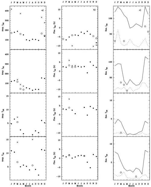
Fig. 2. (a) Relative amplitudes observed. (b) Phase of maxima. Crosses: diurnal tide. Black circles: semidiurnal tide. White circles: less
probable semidiurnal fitting. (c) Residuals. Solid line: before fitting. Dashed line: after the fitting. White circles: after the fitting with a less probable semidiurnal fitting.
in which the solution could be a combination of the diur-nal and the semidiurdiur-nal modulation (because the amplitudes and phases of the diurnal and semidiurnal component do not change much when a combination of both tidal components is considered). The amplitudes and phases, as well as the standard deviation of the data, with respect to their mean value before and after the best fitting, are listed in Table 4 and plotted in Fig. 2.
The diurnal variation of the OH emission rate found throughout the night is similar to that reported from WINDII OH emissions measurements at mid-latitudes (Zhang and Shepherd, 1999; Zhang et al., 2001).
The diurnal tide seems to be consistent with our observa-tions in early spring from both emission rates and tempera-tures, while the semidiurnal tide is predominant for the rest of the year in the O2 emission rate and both temperatures.
This seasonal dependence is in agreement with the seasonal dependence found by Wiens et al. (1995) from ground-based measurements of the O2emission rate and temperature with
the MORTI instrument at 42◦N. They found tidal varia-tions for O2and TO2 to be semidiurnal in winter, diurnal in March and not clearly diurnal or semidiurnal in April. Shep-herd et al. (1995, 1998) also reported a semidiurnal tide at mid-latitude in the Northern Hemisphere during winter sol-stice, determined from the WINDII O(1S) green line emis-sion rates, while at equinoxes the modulation changed to di-urnal. This agrees with the behaviour found from SATI data for the O2 emission rate, and both rotational temperatures,
although from our data the semidiurnal modulations also re-mains in autumn.
Burrage et al. (1995) employed HRDI data and found that the horizontal wind at 95 km is dominated by the semidiurnal
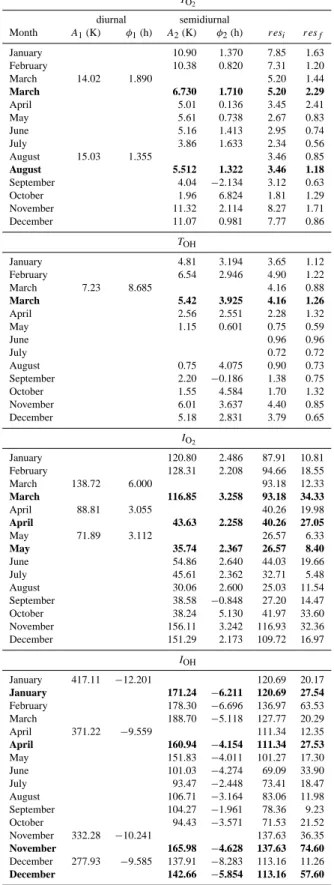
Table 4. Tidal amplitudes and phases that best fit the data
(semidi-urnal tidal solutions with large standard deviations in bold).
TO2
diurnal semidiurnal
Month A1(K) φ1(h) A2(K) φ2(h) resi resf
January 10.90 1.370 7.85 1.63 February 10.38 0.820 7.31 1.20 March 14.02 1.890 5.20 1.44 March 6.730 1.710 5.20 2.29 April 5.01 0.136 3.45 2.41 May 5.61 0.738 2.67 0.83 June 5.16 1.413 2.95 0.74 July 3.86 1.633 2.34 0.56 August 15.03 1.355 3.46 0.85 August 5.512 1.322 3.46 1.18 September 4.04 −2.134 3.12 0.63 October 1.96 6.824 1.81 1.29 November 11.32 2.114 8.27 1.71 December 11.07 0.981 7.77 0.86 TOH January 4.81 3.194 3.65 1.12 February 6.54 2.946 4.90 1.22 March 7.23 8.685 4.16 0.88 March 5.42 3.925 4.16 1.26 April 2.56 2.551 2.28 1.32 May 1.15 0.601 0.75 0.59 June 0.96 0.96 July 0.72 0.72 August 0.75 4.075 0.90 0.73 September 2.20 −0.186 1.38 0.75 October 1.55 4.584 1.70 1.32 November 6.01 3.637 4.40 0.85 December 5.18 2.831 3.79 0.65 IO2 January 120.80 2.486 87.91 10.81 February 128.31 2.208 94.66 18.55 March 138.72 6.000 93.18 12.33 March 116.85 3.258 93.18 34.33 April 88.81 3.055 40.26 19.98 April 43.63 2.258 40.26 27.05 May 71.89 3.112 26.57 6.33 May 35.74 2.367 26.57 8.40 June 54.86 2.640 44.03 19.66 July 45.61 2.362 32.71 5.48 August 30.06 2.600 25.03 11.54 September 38.58 −0.848 27.20 14.47 October 38.24 5.130 41.97 33.60 November 156.11 3.242 116.93 32.36 December 151.29 2.173 109.72 16.97 IOH January 417.11 −12.201 120.69 20.17 January 171.24 −6.211 120.69 27.54 February 178.30 −6.696 136.97 63.53 March 188.70 −5.118 127.77 20.29 April 371.22 −9.559 111.34 12.35 April 160.94 −4.154 111.34 27.53 May 151.83 −4.011 101.27 17.30 June 101.03 −4.274 69.09 33.90 July 93.47 −2.448 73.41 18.47 August 106.71 −3.164 83.06 11.98 September 104.27 −1.961 78.36 9.23 October 94.43 −3.571 71.53 21.52 November 332.28 −10.241 137.63 36.35 November 165.98 −4.628 137.63 74.60 December 277.93 −9.585 137.91 −8.283 113.16 11.26 December 142.66 −5.854 113.16 57.60
tide at latitudes greater than ±40◦. They found that this
semidiurnal variation is larger in winter than in summer. They also found that the semidiurnal tide at 95 km is less evident at the March/April equinox compared to the summer and winter solstices, and even compared to the September equinox. This behaviour is the same as that found here for our O2 emission rate and both rotational temperatures
ob-tained from SATI data. The semidiurnal variation even dis-appears in spring when it becomes predominantly diurnal. In general, the amplitude of the semidiurnal tide, obtained from SATI observations, is greater in winter and autumn than in summer.
The diurnal behaviour of the OH emission rate deduced from SATI data is rather different from that of the O2
emis-sion rates. The diurnal tide for the OH emisemis-sion rate is not only predominant in spring, as for the O2emission rate and
both temperatures, but also seems to be present from late au-tumn to early winter. Although this tidal behaviour of the OH emission rate during winter suggests that the diurnal type of modulation is present, the conclusion has to be considered with caution, because, as can be seen in Table 4, the standard deviation after the fitting is significantly smaller for Decem-ber, while for January the standard deviation after the fitting is very close to that obtained by considering a semidiurnal tidal modulation in fitting of the data. During November the standard deviation after the fitting is greater than the standard deviation obtained after the fitting during the other months of the year. This can indicate that during November other tidal modulations which are not considered here can be present in the nocturnal variation of the OH emission. Bearing in mind that the great variability detected this month could be responsible for this tidal behaviour, this OH tidal behaviour may also indicate that the tidal response of the combination of the tidal responses of the different chemical species in-volved in the chemistry of vibrationally excited OH, mainly atomic hydrogen and ozone, at the altitude of the OH emis-sion peak, is not identical to the combination of the tidal re-sponses of the chemical species involved in the O2(b)
chem-istry, primarily atomic oxygen, at the O2(b)emission peak.
Then, even if the tidal modulations were identical, the ampli-tudes and the phases of these modulations would be different at different altitudes (see L´opez-Gonz´alez et al., 1996, for a model response of the neutral atmosphere to a forced wave modulation). The rotational temperatures deduced from both atmospheric emissions have a similar pattern of variation, in-dicating that, although at different altitudes the tidal pattern of the modulations is the same, the amplitude of the tidal variation is, in general, smaller for the OH temperatures than for the O2temperatures.
The amplitudes and phases of the most probable numerical solution obtained (the one that best fits the data) are plotted in Fig. 2. However, in the cases where the most probable nu-merical solution is the diurnal, we have plotted these ampli-tudes and phases together with those obtained with a possible semidiurnal modulation (also listed in Table 4 with bold char-acters). In these cases the standard deviations of the semidi-urnal modulation are a little greater than those obtained with
ences are not very big and might be indicative that the diurnal solution could be more appropriate, the numerical solution has to be considered with caution.
In the following subsections, for the sake of comparison, we will use the amplitudes and the phases obtained, consid-ering as solution the semidiurnal tidal modulation, even in those cases where the semidiurnal tidal solution is not the one with least standard deviation after the fitting of the data. 3.1 Amplitudes
Figure 2a shows that from late autumn to spring the ampli-tudes of the modulation of both rotational temperatures and emission rates are greater than those during summer. In early spring this modulation seems to be preferentially diurnal in both rotational temperatures and emission rates, while dur-ing the rest of the year this modulation is clearly semidiurnal in both temperatures and O2emission rates, although for the
OH emission rate the semidiurnal modulation seems to be present along with a diurnal modulation from late autumn to early winter.
The amplitudes for the nightly variations of both emission rates and rotational temperatures from November to March were found to be greater than in the rest of the year. Other measurements at mid-latitudes have already yielded a greater amplitude variation in winter (see, e.g. Wiens and Weill, 1973, for OH emission rates at 44◦N and Choi et al., 1998, for OH temperatures and emission rates at 42◦N).
Shepherd and Fricke-Begemann (2004) examined the tem-perature variability in the upper mesosphere, due to migrat-ing tides, by combinmigrat-ing daytime temperature observations of the WINDII satellite experiment with nighttime ground-based potassium lidar measurements at 28◦N. They reported a semidiurnal tidal amplitude of 9 K in November and 4 K in May. From our measurements for 37.06◦N we find an even smaller amplitude in the two data periods, but a larger differ-ence between them, with amplitudes for the semidiurnal tide of 6 K in November and 1 K in May.
From our data we found a semidiurnal tide to be more con-sistent with our November to February observations. The amplitude of the tidal modulation is maximum during these months, about 10–11 K for TO2 and about 5–6 K for TOH. In April the amplitude decreases, reaching an amplitude of 5.6 K for TO2 and 1.1 K for TOH in May. The amplitudes of the semidiurnal modulation also decrease in early sum-mer, although not as much, and remain small in the summer months and early autumn, September–October, until Novem-ber, when a sharp increase in the tidal amplitudes is detected in both emission rates and rotational temperatures. During summer in the TOH data, neither a diurnal nor semidiurnal
tidal modulation is clearly detected (June–July). The stan-dard deviation of the TOHdata before and after the fitting are
nearly the same from May to August, while for the rest of the year the standard deviation after the fitting is smaller than the standard deviation of the data before the fitting, by a factor
the OH temperatures have to be considered with caution. The absolute amplitudes of the O2 emission rate and of
both temperatures are larger by more than a factor of two, and by a somewhat smaller ratio for the OH emission rate variation, from November to February, as compared with the summer months (see Tables 2 and 3).
3.2 Amplitude growth factor
Without energy dissipation the amplitude of a nonevanes-cent wave with upward propagation would grow from the OH to the O2emission layer, as the atmospheric density
de-creases. The observed relative amplitude growth factor in the rotational temperature (defined as the ratio of the relative amplitude of the temperature in the O2and OH layers) has
been calculated using the amplitude obtained for the semid-iurnal tidal solution in all cases, for the sake of comparison (see Table 5). Liu and Swenson (2003) predict for saturated waves (those whose amplitude does not change with the al-titude) a relative amplitude growth factor that goes from 2.2 to 1.0 for waves of vertical wavelength, λz, from 15 km to
50 km (similarly, values from 2.0 to 1.3 for the growth factor of the relative amplitudes of the O2and OH emission rates
are reported for waves with the same vertical wavelength). This ratio is larger for nonevanescent waves (those whose amplitude increases with the altitude) and smaller for waves with larger attenuation. Here we obtain values that are in the range of values predicted by the model of Liu and Swen-son (2003) for nonevanescent waves of vertical wavelength, as detected in the semidiurnal tidal modulations of OH and O2temperatures (Sect. 3.4). The observed amplitude
tem-perature growth factors are greater during May and August but, due to the undetectability or small amplitude variations detected in the OH rotational temperatures from May to Au-gust, the growth temperature factor during these months is affected by large uncertainties, and there is no confidence in the growth factor obtained. Reisin and Scheer (1996) have reported values from 0.9 to 1.7 obtained from observations at mid-latitudes in individual nights, at different times of the year, which are smaller than those obtained here, indicating a stronger wave attenuation in their data on individual nights than those obtained from our monthly mean nocturnal varia-tions.
3.3 Phases
The phases of maxima obtained for both temperatures and emission rates are plotted in Fig. 2b. To make feasible the comparison of the phases we have plotted the phases of max-imum, considering in all cases a semidiurnal modulation as the solution (see Fig. 3). The phase in TO2 temperature is quite stable during the year with maxima in temperature at about one hour after midnight (see Figs. 3a and c). Major changes in the phase of TO2 occur in September and Octo-ber. Also, the phase in the O2emission rate is quite stable
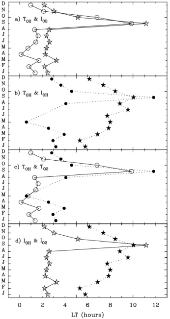
Fig. 3. Phases of maximum. (a) TO2 and IO2. (b) TOHand IOH. (c) TO2 and TOH. (d) IOHand IO2. White circle (solid line): TO2. White star (solid line): IO2. Black circle (dashed line): TOH. Black star (dashed line): IOH.
after midnight. There are exceptions to this stable phase be-haviour, as in the O2temperature, for the months of
Septem-ber and OctoSeptem-ber. It can be seen that the maxima in the O2
emission rates occur about one or two hours later than those in TO2. So, O2temperatures lead the O2emission rates. This pattern is maintained for almost the whole year.
The time of the OH temperature maximum is also rela-tively stable during the year, with a maximum in OH rota-tional temperature at about a mean value of 4 h after midnight (see Figs. 3b and c). Again, large oscillations seem to be ob-tained at the times of the OH temperature maximum during September.
From Fig. 3c it is easy to see that the time of the OH temperature maximum is about 2 h later than the time of the maximum in O2temperature, with the exception of May and
October, where the times of maximum OH temperature lead those of the O2temperature (see Fig. 3c). Thus, with those
exceptions, and bearing in mind that the fitting of OH temper-atures is difficult to detect from May to August (see Fig. 2b and Table 4), O2 rotational temperatures lead OH
tempera-tures for almost the entire year.
Figures 3b and d show that the maximum in the OH emis-sion rate is always later than midnight. The maximum is about 6 h later than midnight from December to February (or 6 h before midnight). This means that OH emission rates reach minimum values close to midnight from December to February. From March to September the maximum values of the OH emission rates move toward later times, from 7 h later than midnight in March to 10 h later than midnight in September (or from 5 to 2 h before midnight, respectively). Then maximum values of OH emission rates move to ear-lier times in the night, as in winter months, from October to November.
The comparison of the times of maximum of the OH emis-sion rates and temperatures shows that the OH emisemis-sion rates reach a maximum about 3–4 h later than the maximum in OH temperatures from August to March, except in September, where the OH emission rate is maximum two hour before that of the OH temperature. During April and May the difference between the time of maximum OH emission rate and tem-perature increases, although it is during these months when it is difficult to find a semidiurnal modulation in OH temper-atures.
The derived semidiurnal parameters from the SATI OH and O2temperature data have been compared with the
semid-iurnal parameters predicted by the Global Scale Wave Model (GSWM) (Hagan et al., 1999). The derived SATI phases of the temperature semidiurnal tide agree very well with those predicted by the GSWM at the respective heights. The OH semidiurnal phases of about 3–4 h local time are in excellent agreement with the GSWM phases predicted for the semid-iurnal tide of about 15–16 h (or 3–4 h) solar local time, at 86.3 km height and 36 N latitude. Similarly, the O2
semid-iurnal tide phases are obtained at about 1–2 h local time, in agreement with the GSWM semidiurnal tide phases of 14– 15 h (or 2–3 h) solar local time at 94.6 km height and 36 N. Further, the change in the OH phase derived from SATI for the month of September is in very good agreement with the GSWM model, while the change in the phase of the O2
semidiurnal tide derived during September-October is pre-dicted earlier in the model, from July to September. Al-though our derived SATI temperature semidiurnal tide am-plitudes are somewhat larger than those predicted by the GSWM model, in general a good agreement is obtained be-tween the SATI derived semidiurnal tide parameters and the parameters predicted by the GSWM model.
The Krassovsky ratio (Krassovsky, 1972) is a complex quan-tity defined as the ratio of the relative amplitudes of the os-cillations in the airglow emission rate and rotational temper-ature. So, the amplitude of the Krassovsky ratio, |η|, is given by: |η| = 1E E 1T T ,
where 1E and 1T are the wave amplitudes detected in the emission rate and in the rotational temperature, and E and T are the average emission rate and rotational temperature. The phase, φ, of Krassovsky’s ratio is given by:
φ = φE−φT,
where φE and φT are the phases of the respective
oscilla-tions in the emission rate and in the temperature, φ is posi-tive when the emission rate oscillation leads the temperature oscillation.
Following the works of Hines and Tarasick (1987), Tara-sick and Hines (1990) and TaraTara-sick and Shepherd (1992a,b) the vertical wavelength, λz, of one perturbation can be
deter-mined from the complex value of the Krassovsky ratio by the expression:
λz∼=
2π γ H
(γ −1)|η| sin φ,
where γ is the ratio of specific heats and H is the scale height. The Krassovsky ratios and the vertical wavelengths found for the semidiurnal tidal oscillation detected from our OH and O2data are listed in Tables 2 and 3, respectively.
For O2emission data |η| values from 3.0 to 9.8 are found
during the year, with 5.9 being the average value. A mean value of 6.9 is obtained from November to March and a mean value of 4.6 is obtained from April to September. For OH emission data greater values of |η| are obtained throughout the year. A mean value of 8.6 is obtained from November to March when strong tidal signatures are present. Greater values are obtained from April to October when the monthly mean amplitudes are smaller than 3 K but those can not be considered very realiable. The phase of η is negative during the year, except during October for O2data (also during May
and September for OH data), indicating an upward energy propagation in the O2 layer throughout the year, except in
October, and an upward energy propagation in the OH layer, except in May and September (although the small ampli-tudes detected in the OH temperature from May to Septem-ber make this result subject to a large uncertainty).
The λzvalues from 18.5 km to 111.8 km are obtained for
O2modulations. A mean value of 33.2 km is obtained from
November to March and 56.9 km from April to September. Smaller values of λz are obtained from the OH data
dur-ing the entire year. A mean value of 16.5 km is obtained for November to March and unrealistic small values are obtained
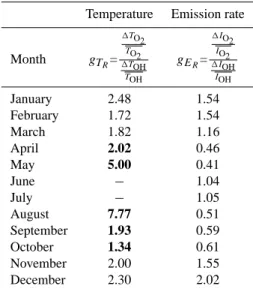
Table 5. Amplitude growth factor. Values obtained from
tempera-ture amplitudes smaller than 3 K in bold.
Temperature Emission rate
Month gTR= 1TO2 TO2 1TOH TOH gER= 1IO2 IO2 1IOH IOH January 2.48 1.54 February 1.72 1.54 March 1.82 1.16 April 2.02 0.46 May 5.00 0.41 June − 1.04 July − 1.05 August 7.77 0.51 September 1.93 0.59 October 1.34 0.61 November 2.00 1.55 December 2.30 2.02
from April to October, when the amplitudes of the tidal vari-ations are the smallest.
For the semidiurnal tide, vertical wavelengths of 36.4 km in the O2layer and of 27.7 km for the OH layer have been
observed by Reisin and Scheer (1996). Values of 27.5 km in the O2layer and of 29 km in the OH layer have been
de-duced from observations taken in February at 37◦N with a modulation of 15 h, and with extreme intensity variations of the O2atmospheric emission (Scheer and Reisin, 1998). In
addition, vertical wavelengths from 12 to 76 km for waves of 3 to 9 h have been observed by Takahashi et al. (1999). Our observations agree with their results.
3.5 Equinox periods
The tidal modulation derived and listed in Table 4 reproduces the data numerically. The standard deviations after the fit-ting are very small and of similar magnitude during the en-tire year, however, larger standard deviations after the fitting seem to remain during October-November for both atures and emission rates and during April for both temper-atures and the O2 emission rate. These differences can be
related to the change in the semidiurnal to diurnal character of the tide during early spring (March–April) and this could also be applied to September and October, although here we find that the semidiurnal tide is dominant during this period. These larger standard deviations after the fitting can be re-lated to the presence of higher tidal harmonics, or greater wave activity. These differences could also be explained by the variations produced in the equinox transition peri-ods. The equinox transition marks two significant periods in the annual variability of the mesosphere and lower ther-mosphere, marked by great activity in winter and more quiet activity period in summer. Shepherd et al. (1999) and Shep-herd et al. (2004b) have discussed the observable effects in
the oxygen airglow during the spring and autumn transitions while Shepherd et al. (2002) and Shepherd et al. (2004a) have discussed the observable effects during the spring and au-tumn transition in the atmospheric temperature.
From the present work, the equinox periods could be char-acterized by:
1. Great changes in the phases of the tidal variations. These changes in the phases of the tidal activity dur-ing the months of September-October could be an in-dication of these transition periods (during March the phases of tidal activity show some changes but not as marked as during the September-October months). 2. During March-April and during September-October a
small growth factor is detected for both temperature amplitudes and emission rate amplitudes, indicating a greater degree of dissipation than during the rest of the year (see Table 5).
3. The fact that large standard deviations after the fitting are obtained for October–November, in both temper-atures and emission rates, and somewhat larger stan-dard deviations after the fitting are present for April, in both temperatures and O2 emission rates, than during
the rest of the year, can be connected to the presence of higher tidal harmonic and wave activity and also with the changes that are produced due to the equinox transi-tions during these periods.
4 Conclusions
The monthly mean diurnal variations for temperatures and emission rates, deduced from the OH(6-2) Meinel and O2
(0-1) atmospheric bands at a latitude of 37.06◦N, from SATI operation in 1998 to 2003, have been presented. A clear daily modulation is found in temperatures and emission rates:
– The modulation is predominantly semidiurnal in both
temperatures and emission rates throughout the year.
– During spring the semidiurnal variation changes to a
di-urnal type, in both temperature and emission rates.
– During late autumn and early winter OH emission rates
show both diurnal and semidiurnal modulations. From summer to late autumn the amplitudes of the diurnal variation decrease by more than a factor of two compared with those in winter and spring.
Mean vertical wavelengths for the semidiurnal modulation of 33.2 km in the O2layer and of 16.5 km for the OH layer
are obtained from November to March with our data. A clear upward energy propagation is observed during most of the year, with some indication of possible downward energy propagation close to the equinoxes.
Both emission rates and rotational temperatures present a similar pattern of diurnal variation throughout the year, yield-ing maximum values some time after midnight.
It is clear that, in general, TO2leads the O2emission rates, that O2 rotational temperatures also lead the OH rotational
temperatures and that TOHleads the OH emission rates. Both
emission rates have phase shifts from about 3 h to 7 h (−5 h) for the entire year, with the O2emission rate leading the OH
emission rate, expect in July, August and September, when the OH emission rate leads the O2emission rate.
Acknowledgement. This research was partially supported by the
Di-recci´on General de Investigaci´on (DGI) under projects AYA2000-1559 and AYA2003-04651, the Comisi´on Interministerial de Cien-cia y Tecnolog´ıa under projects REN2001-3249 and ESP2004– 01556, the Junta de Andaluc´ıa, NATO under a Collaborative Link-age Grants 977354 and 979480 and INTAS under the research project 03-51-6425. We very gratefully acknowledge the staff of Sierra Nevada Observatory for their help and assistance with the SATI instrument. We wish to thank the referee for useful comments and suggestions.
Topical Editor U. P. Hoppe thanks a referee for his/her help in evaluating this paper.
References
Abreu, V. J. and Yee, J. H.: Diurnal and seasonal variation of the nighttime OH(8-3) emission at low latitudes, J. Geophys. Res., 94, 11 949–11 957, 1989.
Burrage, M. D., Arvin, N., Skinner, W. R., and Hays, P. B.: Obser-vations of the O2atmospheric band nightglow by the High
Res-olution Doppler Imager, J. Geophys. Res., 99, 15 017–15 023, 1994.
Burrage, M. D., Wu, D. L., Skinner, W. R., Ortland, D. A., and Hays, P. B.: Latitude and seasonal dependence of the semidiurnal tide observed by the high-resolution Doppler imager, J. Geophys. Res., 100, 11 313–11 321, 1995.
Crary, J. D. and Forbes, J. M.: On the extraction of tidal information from measurements covering a fraction of a day, Geophys. Res. Lett., 10, 580–582, 1983.
Chapman, S. and Lindzen, R. S.: Atmospheric tides: thermal and gravitational, Gordon and Breach, New York, 1–23, 1970. Choi, G. H., Monson, I. K., Wickwar, V. B., and Rees, D.:
Sea-sonal and diurnal variations of wind and temperature near the mesopause from Fabry-Perot interferometer observations of OH Meinel emissions, Adv. Space Res., 21, 847–850, 1998. Forbes, J. M., Portnyagin, Yu. I., Skinner, W., Vincent, R. A.,
Solovjova, T., Merzlyakov, E., Nakamura, T., and Palo, S.: Cli-matological lower thermosphere winds as seen by ground-based and space-based instruments, Ann. Geophys., 22, 1931–1945, 2004,
SRef-ID: 1432-0576/ag/2004-22-1931.
Hagan, M. E., Burrage, M. D., Forbes, J. M., Hackney, J., Randel, W. J., and Zhang, X.: GSWM-98: Results for migrating solar tides, J. Geophys. Res., 104, 6813–6828, 1999.
Hines, C. O. and Tarasick, D. W.: On the detection and utilization of gravity waves in airglow studies, Planet. Space Sci., 35, 851– 866, 1987.
Jacobi, Ch., Portnyagin, Yu. I., Solovjova, T. V., Hoffmann, P., Singer, W., Fahrutdinova, A. N., Ishmuratov, R. A., Beard, A. G., Mitchell, N. J., Muller, H. G., Schminder, R., K¨urschner, D., Manson, A. H., and Meek, C. E.: Climatology of the semidiur-nal tide at 52–56 N from ground-based radar wind measurements 1985–1995, J. Atmos. Solar-Terr. Phys., 61, 975–991, 1999.
atmosphere, Ann. Geophys., 28, 739–746, 1972.
Liu, A. Z. and Swenson, G. R.: A modeling study of O2and OH airglow perturbations induced by atmospheric gravity waves, J. Geophys. Res., 108(D4), 4151, doi:10.1029/2002JD2474, 2003. L´opez-Gonz´alez, M. J., Murtagh, D. P., Espy, P. J., L´opez-Moreno, J. J., Rodrigo, R., and Witt, G.: A model study of the temporal behaviour of the emission intensity and rotational temperature of the OH Meinel bands for high-latitude summer conditions, Ann. Geophys., 14, 59–67, 1996,
SRef-ID: 1432-0576/ag/1996-14-59.
L´opez-Gonz´alez, M. J., Rodr´ıguez, E., Wiens, R. H., Shepherd, G. G., Sargoytchev, S., Brown, S., Shepherd, M. G., Aushev, V. M., L´opez-Moreno, J. J., Rodrigo, R., and Cho, Y.-M.: Seasonal variations of O2Atmospheric and OH(6-2) airglow and
temper-ature at mid-latitudes from SATI observations, Ann. Geophys., 22, 819–828, 2004,
SRef-ID: 1432-0576/ag/2004-22-819.
Manson, A. H., Meek, C. E., Chshyolkova, T., Avery, S. K., Thorsen, D., MacDougall, J. W., Hocking, W., Murayama, Y., Igarashi, K., Namboothiri, S. P., and Kishore, P.: Longitudinal and latitudinal variations in dynamic characteristics of the MLT (70–95 km): a study involving the CUJO network, Ann. Geo-phys., 22, 347–365, 2004,
SRef-ID: 1432-0576/ag/2004-22-347.
Pancheva, D., Mukhtarov, P., Mitchell, N. J., Beard, A. G., and Muller, H. G.: A comparative study of winds and tidal variability in the mesosphere/lower-thermosphere region over Bulgaria and the UK, Ann. Geophys., 18, 1304–1315, 2000,
SRef-ID: 1432-0576/ag/2000-18-1304.
Pancheva, D., Merzlyakov, E., Mitchell, N. J., Portnyagin, Yu., Manson, A. H., Jacobi, Ch., Meek, C. E., Luo, Y., Clark, R. R., Hocking, W. K., MacDougall, J., Muller, H. G., K¨urschner, D., Jones, G. O. L., Vincent, R. A., Reid, I. M., Singer, W., Igarashi, K., Fraser, G. I., Fahrutdinova, A. N., Stepanov, A. M., Poole, L. M. G., Malinga, S. B., Kashcheyev, B. L., and Oleynikov, A. N.: Global-scale tidal variability during the PSMOS campaign of June–August 1999: interaction with planetary waves, J. Atmos. Solar-Terr. Phys., 64, 1865–1896, 2002.
Pendleton Jr., W. R. and Taylor, M. J.: The impact of L-uncoupling on Einstein coefficients for the OH Meinel (6,2) band: implica-tions for Q-branch rotational temperatures, J. Atmos. Solar-Terr. Phys., 64, 971–983, 2002.
Petitdidier, M. and Teitelbaum, H.: Lower thermosphere emissions and tides, Planet. Space Sci., 25, 711–721, 1977.
Portnyagin, Y. I., Solovjova, T. V., Makarov, N. A., Merzlyakov, E. G., Manson, A. H., Meek, C. E., Hocking, W., Mitchell, N., Pancheva, D., Hoffmann, P., Singer, W., Murayama, Y., Igarashi, K., Forbes, J. M., Palo, S., Hall, C., and Nozawa, S.: Monthly mean climatology of the prevailing winds and tides in the Arc-tic mesosphere/lower thermosphere, Ann. Geophys., 22, 3395– 3410, 2004,
SRef-ID: 1432-0576/ag/2004-22-3395.
Reisin, E. R. and Scheer, J.: Characteristics of atmospheric waves in the tidal period range derived from zenith observations of O2
(0-1) Atmospheric and OH(6-2) airglow at lower midlatitudes, J. Geophys. Res., 101, 21 223–21 232, 1996.
Riggin, D. M., Meyer, C. K., Fritts, D. C., Jarvis, M. J., Murayama, Y., Singer, W., Vincent, R. A., and Murphy, D. J.: MF radar observations of seasonal variability of semidiurnal motions in the mesosphere at high northern and southern latitudes, J. Atmos. Solar-Terr. Phys., 65, 483–493, 2003.
G. G., and L´opez-Gonz´alez, M. J.: Spectral airglow temperature imager (SATI) – a ground based instrument for temperature mon-itoring of the mesosphere region, Appl. Opt., 43, 5712–5721, 2004.
Scheer, J. and Reisin, E. R.: Rotational temperatures for OH and O2 airglow bands measured simultaneously from El Leoncito
(31◦480S), J. Atmos. Terr. Phys., 52, 47–57, 1990.
Scheer, J. and Reisin, E. R.: Extreme intensity variations of O2b
airglow induced by tidal oscillations, Adv. Space Res., 21, 827– 830, 1998.
Shepherd, M. G. and Fricke-Begemann, C.: Study of the tidal vari-ations in mesospheric temperature at low and mid latitudes from WINDII and potassium lidar observations, Ann. Geophys., 22, 1513–1528, 2004,
SRef-ID: 1432-0576/ag/2004-22-1513.
Shepherd, G. G., McLandress, C., and Solheim, B. H.: Tidal in-fluence on O(1S) airglow emission rate distributions at the ge-ographic equator as observed by WINDII, Geophys. Res. Lett., 22, 275–278, 1995.
Shepherd, G. G., Roble, R. G., Zhang, S. P., McLandress, C., and Wiens, R. H.: Tidal influences on midlatitude airglow: Compari-son of satellite and ground-based observations with TIME-GCM predictions, J. Geophys. Res., 103, 14 741–14 751, 1998. Shepherd, G. G., Stegman, J., Espy, P., McLandress, C., Thuillier,
G., and Wiens, R. H.: Springtime transition in lower thermo-spheric atomic oxygen, J. Geophys. Res., 104, 213–223, 1999. Shepherd, M. G., Espy, P. J., She, C. Y., Hocking, W., Keckhut,
P., Gavrilyeva, G., Shepherd, G. G., and Naujokat, B.: Spring-time transition in upper mesospheric temperature in the Northern Hemisphere, J. Atmos. Solar-Terr. Phys., 64, 1183–1199, 2002. Shepherd, M. G., Rochon, Y. I., Offermann, D., Donner, M., and
Espy, P. J.: Longitudinal variability of mesospheric temperatures during equinox at middle and high latitudes, J. Atmos. Solar-Terr. Phys., 66, 463–479, 2004a.
Shepherd, G. G., Stegman, J., Singer, W., and Roble, R. G.: Equinox transition in wind and airglow observations, J. Atmos. Solar-Terr. Phys., 66, 481–491, 2004b.
Takahashi, H., Sahai, Y., Clemesha, B. R., Batista, P. P., and Teix-eira, N. R.: Diurnal and seasonal variations of the OH (8,3) air-glow band and its correlation with OI 5577, Planet. Space Sci., 25, 541–547, 1977.
Takahashi, H., Gobbi, D., Batista, P. P., Melo, S. M. L., Teixeira, N. R., and Buriti, R. A.: Dynamical influence on the equatorial airglow observed from the South American sector, Adv. Space Res., 21, 817–825, 1998.
Takahashi, H., Batista, P. P., Buriti, R. A, Gobbi, D., Nakamura, T. Tsuda, T., and Fukao, S.: Response of the airglow OH emission, temperature and mesopause wind to the atmospheric wave prop-agation over Shigaraki, Japan, Earth Planets Space, 51, 863–875, 1999.
Tarasick, D. W. and Hines, C. O.: The observable effects of gravity waves on airglow emissions, Planet. Space Sci., 38, 1105–1119, 1990.
Tarasick, D. W. and Shepherd, G. G.: Effects of gravity waves on complex airglow chemistries. 1 O2(b16+g)emission, J.
Geo-phys. Res., 97, 3185–3193, 1992a.
Tarasick, D. W. and Shepherd, G. G.: Effects of gravity waves on complex airglow chemistries. 2. OH emission, J. Geophys. Res., 97, 3195–3208, 1992b.
Wiens, R. H. and Weill, G.: Diurnal, annual and solar cycle variations of hydroxyl and sodium nightglow intensities in the
Europe-Africa sector, Planet. Space Sci., 21, 1011–1027, 1973. Wiens, R. H., Zhang, S. P., Peterson, R. N., and Shepherd, G. G.:
MORTI: A Mesopause Oxygen Rotational Temperature Imager, Planet. Space Sci., 39, 1363–1375, 1991.
Wiens, R. H., Zhang, S. P., Peterson, R. N., and Shepherd, G. G.: Tides in emission rate and temperature from O2nightglow over
Bear Lake Observatory, Geophys. Res. Lett., 22, 2637–2640, 1995.
Wiens, R. H., Moise, A., Brown, S., Sargoytchev, S., Peterson, R. N., Shepherd, G. G., L´opez-Gonz´alez, M. J., L´opez-Moreno, J. J., and Rodrigo, R.: SATI: A Spectral Airglow Temperature Im-ager, Adv. Space Res., 19, 677–680, 1997.
Zhang, S. P. and Shepherd, G. G.: The influence of the diurnal tide on the O(1S) and OH emission rates observed by WINDII on UARS, Geophys. Res. Lett., 26, 529–532, 1999.
Zhang, S. P., Shepherd, G. G., and Roble, R. G.: Tidal influence on the oxygen and hydroxyl nightglows: Wind Imaging Interfer-ometer observations and thermosphere/ionosphere/mesosphere electrodynamics general circulation model, J. Geophys. Res., 106, 21 381–21 393, 2001.