Stratospheric temperatures and tracer transport in a nudged 4-year middle atmosphere GCM simulation

(1)

HAL Id: hal-00301035

https://hal.archives-ouvertes.fr/hal-00301035

Submitted on 21 Feb 2005

HAL is a multi-disciplinary open access

archive for the deposit and dissemination of sci-entific research documents, whether they are pub-lished or not. The documents may come from teaching and research institutions in France or abroad, or from public or private research centers.

L’archive ouverte pluridisciplinaire HAL, est destinée au dépôt et à la diffusion de documents scientifiques de niveau recherche, publiés ou non, émanant des établissements d’enseignement et de recherche français ou étrangers, des laboratoires publics ou privés.

Stratospheric temperatures and tracer transport in a

nudged 4-year middle atmosphere GCM simulation

M. K. van Aalst, J. Lelieveld, B. Steil, C. Brühl, P. Jöckel, M. A. Giorgetta,

G.-J. Roelofs

To cite this version:

M. K. van Aalst, J. Lelieveld, B. Steil, C. Brühl, P. Jöckel, et al.. Stratospheric temperatures and tracer transport in a nudged 4-year middle atmosphere GCM simulation. Atmospheric Chemistry and Physics Discussions, European Geosciences Union, 2005, 5 (1), pp.961-1006. �hal-00301035�

(2)

ACPD

5, 961–1006, 2005 Stratospheric temperatures and transport in a nudged GCM

M. K. van Aalst et al.

Title Page Abstract Introduction Conclusions References Tables Figures J I J I Back Close

Full Screen / Esc

Print Version Interactive Discussion

EGU Atmos. Chem. Phys. Discuss., 5, 961–1006, 2005

www.atmos-chem-phys.org/acpd/5/961/ SRef-ID: 1680-7375/acpd/2005-5-961 European Geosciences Union

Atmospheric Chemistry and Physics Discussions

Stratospheric temperatures and tracer

transport in a nudged 4-year middle

atmosphere GCM simulation

M. K. van Aalst1, J. Lelieveld2, B. Steil2, C. Br ¨uhl2, P. J ¨ockel2, M. A. Giorgetta3, and G.-J. Roelofs1

1

Institute for Marine and Atmospheric Research (IMAU), Utrecht, The Netherlands 2

Max Planck Institute for Chemistry, Mainz, Germany 3

Max Planck Institute for Meteorology, Hamburg, Germany

Received: 6 January 2005 – Accepted: 12 February 2005 – Published: 21 February 2005 Correspondence to: M. K. van Aalst (maarten.vanaalst@xs4all.nl)

(3)

ACPD

Full Screen / Esc

EGU

Abstract

We have performed a 4-year simulation with the Middle Atmosphere General Circu-lation Model MAECHAM5/MESSy, while slightly nudging the model’s meteorology in the free troposphere (below 113 hPa) towards ECMWF analyses. We show that the nudging technique, which leaves the middle atmosphere almost entirely free, enables

5

comparisons with synoptic observations. The model successfully reproduces many specific features of the interannual variability, including details of the Antarctic vortex structure. In the Arctic, the model captures general features of the interannual vari-ability, but falls short in reproducing the timing of sudden stratospheric warmings. A detailed comparison of the nudged model simulations with ECMWF data shows that

10

the model simulates realistic stratospheric temperature distributions and variabilities, including the temperature minima in the Antarctic vortex. Some small (a few K) model biases were also identified, including a summer cold bias at both poles, and a general cold bias in the lower stratosphere, most pronounced in midlatitudes. A comparison of tracer distributions with HALOE observations shows that the model successfully

15

reproduces specific aspects of the instantaneous circulation. The main tracer trans-port deficiencies occur in the polar lowermost stratosphere. These are related to the tropopause altitude as well as the tracer advection scheme and model resolution. The additional nudging of equatorial zonal winds, forcing the quasi-biennial oscillation, sig-nificantly improves stratospheric temperatures and tracer distributions.

20

1. Introduction

Van Aalst et al. (2004a) applied a Newtonian relaxation technique in a middle atmo-sphere (MA) general circulation model (GCM) to nudge the model towards meteoro-logical analyses for a particular period. Van Aalst et al. (submitted, 2004b)1 showed

1

Van Aalst, M. K., Lelieveld, J., Steil, B., Br ¨uhl, C., J ¨ockel, P., Kirchner, I., and Roelofs, G.-J.: The 2002 Antarctic vortex split in a nudged middle-atmosphere GCM, Geophys. Res. Lett.,

(4)

ACPD

Full Screen / Esc

EGU that their GCM, MAECHAM5 (ECHAM5 is the European Centre Model, Hamburg

ver-sion 5), reproduces the unprecedented Antarctic vortex split in September 2002 when nudging only the lower part of the model (below 113 hPa) towards analyses of the Eu-ropean Centre for Medium-range Weather Forecasts (ECMWF). They noted that this result offers good prospects for direct comparisons of model results with synoptic

ob-5

servations, while leaving the middle atmosphere entirely free, as in the free-running GCM.

With the current simulations we have tested this setup for a 4-year period to examine temperature distributions and tracer transports in the stratosphere. While these sim-ulations employ the a version of MAECHAM5/MESSy (MESSy is the Modular Earth

10

Submodel System; seehttp://www.messy-interface.org) without comprehensive chem-istry, our analysis addresses the potential to apply this nudging technique in a GCM with fully coupled chemistry (e.g. Steil et al., 2003; Manzini et al., 2003). Our focus is primarily on (i) the degree to which polar dynamical processes approximate reality, in-cluding the occurrence and timing of sudden stratospheric warmings and the location of

15

the polar vortex; (ii) the accuracy of simulated stratospheric temperatures, particularly in the polar regions, for instance to realistically represent Polar Stratospheric Cloud (PSC) conditions; and (iii) large-scale tracer transports (diagnosed by comparing mod-eled methane and water vapor fields with satellite observations). While we leave most of the middle atmosphere entirely free, we also force a realistic quasi-biennial

oscilla-20

tion (QBO) by applying a weak nudging to the stratospheric equatorial zonal wind. The QBO nudging allows to include the QBO and its effects on temperature and transport even though the vertical resolution used here is too coarse to simulate the QBO di-rectly (Giorgetta et al., 2002). Furthermore, this assimilation, which follows observed time series, also allows the synchronization of the QBO with the weather assimilated in

25

the troposphere and with prescribed sea surface temperatures and ice concentrations. Our simulations can be compared to more regular assessments of GCM perfor-mance, which usually focus on averages and variabilities over longer time periods,

(5)

ACPD

Full Screen / Esc

EGU comparing at least 10–15 years of output from free-running GCMs with

meteorologi-cal reanalysis datasets and/or climatologies based on a similarly long record of mea-surements. This has several drawbacks. First, the atmospheric background chemical conditions are not constant due to changing emissions, particularly of long-lived green-house gases and chlorofluorocarbons that affect stratospheric ozone and dynamics.

5

Steady-state “time slice” GCM simulations (e.g. Steil et al., 2003; Manzini et al., 2003) do not capture these trends, and cannot be compared to sufficiently long sets of at-mospheric data (particularly when the primary interest of the GCM simulations is to study processes that are sensitive to the changes induced by the changes in atmo-spheric composition). An alternative is to use so-called transient GCM experiments

10

(e.g. Austin, 2002), which explicitly include the changing emissions. While these simu-lations are valuable to analyze long-term trends, a difficulty is that the transient runs are associated with internal, e.g. interannual variability, complicating detailed comparisons with measurements. Furthermore, for many processes and parameters long measure-ment records are not available, thus precluding a statistical analysis. Finally, it may be

15

desirable to simulate particular measurement campaigns.

The nudging applied here provides a simple tool to assess the performance of a regular GCM (in this case including the middle atmosphere, potentially also includ-ing coupled chemistry) while retaininclud-ing the full consistency and flexibility of the climate model, as it is also used for free-running climate simulations. While it is possible to

20

apply the nudging technique in the entire domain for which analyses are available (as in Van Aalst et al., 2004a), it is desirable to limit the nudging to the extent possible (as in Van Aalst et al., submitted, 2004b1) to prevent that model errors are masked by artificial tendencies, and also because in some cases the model may actually outper-form the analyses, particularly when the model is applied with coupled chemistry, and

25

in areas where observations are sparse (in most of the middle atmosphere).

Section 2 briefly describes the MAECHAM5/MESSy model and the setup of our nudged simulations. Section 3 discusses the analyses and observations used in our comparisons. Sections 4 and 5 evaluate the main results for temperatures and tracer

(6)

ACPD

Full Screen / Esc

EGU fields, and Sects. 6 and 7 present the discussion and conclusions.

2. Model description and nudging

MAECHAM5/MESSy is the middle atmosphere configuration of the ECHAM5 GCM described by Roeckner et al. (2003), with extensions from the Modular Earth Sub-model System (MESSy) (J ¨ockel et al., 2004). MAECHAM5 includes all processes of

5

the tropopheric ECHAM5 and computes additionally the momentum deposition in the middle atmosphere by the dissipation of a vertically propagating spectrum of gravity waves of tropospheric origin. The gravity wave scheme has been implemented in the previous model version, MAECHAM4 (Manzini and McFarlane, 1998; Manzini et al., 1997) for the previous model version (MAECHAM4). The latter has been used

exten-10

sively for a variety of studies, including those with coupled chemistry (e.g. Steil et al., 2003; Manzini et al., 2003). MAECHAM5 has been applied by Giorgetta et al. (2002), who showed that the model (in the 90-level configuration) successfully simulates the QBO, and Manzini et al. (submitted, 2004)2, who assessed the influence of sea surface temperatures on the Northern winter stratosphere.

15

In our current simulations, we have used a similar model setup as in Van Aalst et al. (submitted, 2004b)1, with a spectral triangular truncation at T42, which corresponds to a horizontal resolution of about 2.8 by 2.8◦ longitude-latitude. Tracer transport is calculated with a flux-form semi-Lagrangian advection (FFSL) scheme (Lin and Rood, 1996); we also performed sensitivity runs with the semi-Lagrangian Transport (SLT)

20

scheme (Rasch and Williamson, 1990; Rasch et al., 1995), which was the standard scheme in ECHAM4, and the Split Implementation of Transport Using Flux Integral Representation (SPITFIRE) advection scheme (Rasch and Lawrence, 1998), which

2

Manzini, E., Giorgetta, M. A., Kornblueh, L., and Roeckner, E.: The influence of sea surface temperatures on the Northern winter stratosphere: Ensemble simulations with the MAECHAM5 model, J. Clim., submitted, 2004.

(7)

ACPD

Full Screen / Esc

EGU was used in MAECHAM4 by Steil et al. (2003). The time step is 900 s; full radiation

calculations are performed every 8 time steps (2 h).

The nudging setup is similar to the standard runs of Van Aalst et al. (submitted, 2004b)1. Full nudging, with a relaxation time scale of 48 h for the divergence, 24 h for temperature and surface pressure, and 6 h for vorticity (as in Guldberg and Kaas,

5

2000), is applied between level 7 and level 27 (corresponding to about 223 hPa and about 690 hPa for locations without orography, respectively), with the nudging tapering off exponentially in the three levels above and below (at 50, 25, and 12.5% of the full strength, respectively). No nudging is applied above level 24 (113 hPa). To avoid the excitation of spurious gravity waves, the ECMWF data were interpolated to the model

10

grid using a state-of-the-art interpolation scheme, and subsequently filtered by project-ing them onto the model normal modes, and filterproject-ing out all components faster than 24 h. Even without this slow-normal-mode filtering, our nudging settings have been shown to create minimal artificial forcings in the model (Guldberg and Kaas, 2000). Sea surface temperatures are prescribed consistently from the ECMWF analyses.

15

In addition to the global nudging in spectral space, our standard simulations also in-cluded the MESSy submodel QBO, a nudging of the quasi-biennial oscillation (QBO). The QBO substantially influences the large-scale dynamics and tracer transports in the middle atmosphere (and indirectly also in the troposphere) (Baldwin et al., 2001). Hence, a comparison of our model with the actual atmosphere in a particular period

20

requires a realistic phase of the QBO. However, the low vertical resolution used here because of practical constraints does not allow the direct simulation of the QBO (Gior-getta et al., 2002), so that the QBO is forced externally by assimilation of the observed QBO (as in Giorgetta and Bengtsson, 1999, similar to other GCM experiments with QBO assimilation, such as by Hamilton, 1998). This QBO assimilation consists of a

25

Newtonian relaxation of the zonal wind in the QBO domain towards an idealized QBO that (a) is zonally uniform, (b) has a latitudinal Gaussian bell shape centered on the equator, and (c) evolves in time as observed in wind data from Singapore (1◦N,104◦E) (Naujokat, 1986; Marquardt and Naujokat, 1997). The original observations (up to

(8)

ACPD

Full Screen / Esc

EGU 10 hPa) were extended to 3 hPa using a backward running propagation operator that

exploits the observed regularity in the QBO propagation. This nudging is applied with a relaxation timescale of a week (at the center of the QBO nudging domain, tapering off towards 20◦ latitude north and south, and towards the top and bottom of the QBO nudging domain, at 3 and 100 hPa). This timescale (as in Hamilton, 1998) is sufficient

5

to force the correct QBO phase but leaves the model full freedom to develop its own dynamics on shorter timescales.

The middle atmospheric methane and water vapor fields were updated according to MESSy submodel H2O, in a similar way as Van Aalst et al. (submitted, 2004b)1. Methane and water vapor above 100 hPa are initialized using a bimonthly zonal mean

10

climatology prepared from four years (1993–1996) of data from the Halogen Occulta-tion Experiment (HALOE) instrument aboard the Upper Atmosphere Research Satellite (UARS) (see below). Tropospheric methane is set at 1.75 ppmv (distributed over the hemispheres). After initialization, methane is advected as a model tracer, while surface concentrations are kept constant. Methane loss and H₂O production are simulated by

15

applying monthly zonal mean methane loss fields for reactions with OH, Cl, and O(1D), taken from a chemistry-climate run with MAECHAM4/CHEM (Steil et al., 2003). Pho-todissociation of methane and water vapor, and reaction of water vapor with O(1D) are not included, which results in a slight high bias of both tracers in the mesosphere. CO₂ and tropospheric N₂O are fixed at 372 ppmv and 320 ppbv, respectively (WMO,

20

1999). We have used tropopause diagnostics from the MESSy submodel TROPOP, which uses a combination of the WMO tropopause definition (as in Reichler et al., 2003; Dameris et al., 1995) and a dynamic PV criterion (2 K m2/kg/s).

Our simulations included the period from May 1999 to October 2003, with the first months considered as spin-up for the nudging and the tracer fields. Hence, we

ob-25

tained essentially four years of model data, including four Arctic and three Antarctic winters, to compare to analyzed temperatures and tracer observations. Besides the base run (with tropospheric and QBO nudging), we performed similar runs without the QBO nudging, and also without the tropospheric nudging. In addition, we performed

(9)

ACPD

Full Screen / Esc

EGU shorter (20 months) sensitivity runs with the SLT and SPITFIRE advection schemes,

with the FFSL scheme with a surface pressure mass mismatch fixer, and with the FFSL scheme at higher resolution (spectral triangular truncation T63, corresponding to about 1.875×1.875◦latitude-longitude).

3. Analyses and observations

5

3.1. ECMWF data

Operational analyses from the ECMWF were used as input for the nudging (at alti-tudes below 113 hPa) and for comparisons with model temperatures at 70, 50, 30 and 10 hPa. Lower stratospheric ECMWF analyses have been shown to agree well with sonde and satellite measurements, particularly also in the polar regions. For

in-10

stance, Pommereau et al. (2002) and Knudsen et al. (2002) found a minor warm bias of 0.49 K with a standard deviation of 0.91 K in comparisons with independent long-duration balloon observations for Arctic winter temperatures below 30 hPa in the (rela-tively cold) winter 1999/2000. Similarly, Hertzog et al. (2004) found a cold bias of about 0.3 K with a standard deviation of 0.8 K at 70 hPa in the 2001/2002 Arctic winter, and

15

Knudsen (2003), using data up to 11 hPa from 1999/2000, 2002/2003 and 1996/1997 (ECMWF ERA reanalysis data for the latter) found biases generally well below 1 K, except in the 11–26 hPa layer during the 2002/2003 winter, which showed a cold bias of 1.05±1.17 K. While Manney et al. (2003) found large differences in PSC coverage between various meteorological analyses, Knudsen (2002) has shown that below 26

20

hPa, the analyzed temperatures below T_NAT are within 10% of those observed by radio sondes (i.e. within the error margins). Above 26 hPa however, the ECMWF analyses almost always overestimate the area PSC coverage. At these higher altitudes, the ECMWF temperatures generally become rather uncertain, given the paucity of obser-vations for assimilation.

25

(10)

im-ACPD

Full Screen / Esc

EGU proved over time as new model versions have been released and additional satellite

observations have been assimilated (Simmons et al., 2005). During the entire 4-year period simulated here, the ECMWF used a model with a top level at 0.1 hPa, with 50 vertical levels until 12 October 1999, and 60 levels thereafter. The horizontal reso-lution was T319 until 21 November 2000 and T511 thereafter, corresponding to grid

5

sizes of about 60 and 40 km, respectively. A slight temperature error may have oc-curred in the lower stratosphere between October 1999 and 10 April 2000 due to an error in the humidity fields in a shallow layer just above the tropopause in this period (ECMWF website http://www.ecmwf.int, model version history). Shifts in the quality of the analyzed fields could partly be avoided by using reanalysis data, such as from

10

ERA-40 (Simmons and Gibson, 2000), which do suffer from instrument and converge discontinuities, but not from changes in model versions.

3.2. HALOE observations

We have used methane and water vapor data from the Halogen Occultation Experi-ment (HALOE) instruExperi-ment aboard the Upper Atmosphere Research Satellite (UARS)

15

(Russell et al., 1993). Park et al. (1996) estimated that the total error in methane is within 15% and the precision is better than 7% over the 1 to 100 hPa height range. Harries et al. (1996) found that the accuracy of the HALOE H₂O observations is within 10% between 0.1 and 100 hPa, and within 30% at the boundaries of its observational range (from the tropopause to about 0.002 hPa). In the lower stratosphere, the

preci-20

sion is a few percent. For both methane and water vapor the vertical resolution is about 2 km. In this study, we have used the version 19 data (available at the HALOE website http://haloedata.larc.nasa.gov), which should have an improved accuracy compared to the version 17 products used in the validation papers, particularly in the lower parts of the observational range.

25

The HALOE data are used in two ways. As noted above, the MESSy submodel H2O initializes our water vapor and methane fields (above 100 hPa) with a climato-logy of HALOE data (compiled in 1993–1996). Secondly, we have used HALOE

(11)

mea-ACPD

Full Screen / Esc

EGU surements from the period that was simulated in our experiments to test the model

representation of tracer transports.

4. Results: temperatures

4.1. Antarctic and Arctic

Figure 1 shows a comparison of temperatures from MAECHAM5/MESSy with those

5

from ECMWF analyses, at 80◦S, 10 and 70 hPa. Similar analyses were examined for 30 and 50 hPa (as discussed below), for the pole region and 70◦ latitude (with very similar results as at 80◦). For each month, we collected the temperatures at all grid points along the latitude band (using 12-hourly data, for both ECMWF and MAECHAM5/MESSy). The figure shows the monthly median and mean temperatures,

10

as well as the 33 and 66 percentiles and the minimum and maximum temperatures, thus providing an impression of the distribution and variability of both our model and the higher resolution analyses.

The figure shows that the model accurately captures the interannual variability, es-pecially of the lowest temperatures reached in the Antarctic vortex, including the cold

15

winter minimum of 2003. During each winter, the model captures the temperature de-velopment, as well as the variability in the monthly datasets (minima and maxima as well as standard deviations or 33/66 percentiles).

This is confirmed by Fig. 2, which shows the fractional area south of 50◦S with temperatures lower than 190 K (integral calculated for each month, based on 12-hourly

20

data), at 89, 70 and 54 hPa, as an indication of the model’s ability to simulate the extent of very low temperatures required for the formation of PSCs, which promote chlorine activation and ozone destruction. At 89 hPa, MAECHAM5/MESSy has a small cold bias, but at 54 and 70 hPa (the altitude of largest ozone loss), the model performs re-latively well. Table 1 shows the relative difference between MA-ECHAM5 and ECMWF

25

(12)

ACPD

Full Screen / Esc

EGU month. MAECHAM5/MESSy tends to overestimate the area colder than 190 K at 54

and 70 hPa by about 10%, except in 2001, where it simulates a substantially larger cold area than the ECMWF analysis. The model reproduces the relatively warm 2002 winter quite well.

Relatively larger differences between MAECHAM5/MESSy and the ECMWF

analy-5

ses occur at the end of the Southern winter, particularly in the area between 50 and 70 hPa. The mean temperature in MAECHAM5/MESSy increases more rapidly than in the ECMWF analyses, and the area with temperatures below 190 K decreases too rapidly, except in late winter 2002. This relative warming can be explained by the use of the Fortuin and Kelder (1998) ozone climatology, which is representative for conditions

10

in the late 1980s, when the ozone hole was much smaller. When sunlight returns to the pole, the climatology’s overestimate of ozone concentrations results in too much absorption of solar radiation and accelerated warming. This explanation complies with the better model performance for 2002, after an unusually disturbed winter with a re-latively weak ozone hole after the vortex breakup in September. Note that this rapid

15

warming tendency is expected to vanish in simulations with coupled chemistry, which will generate more realistic ozone concentrations in the Antarctic vortex. Indeed, Steil et al. (2003) found that simulations with coupled chemistry generally simulated a shift to lower average temperatures at the South Pole ranging from 5–10 K in October to 10–14 K in November. GCM simulations without coupled chemistry should thus use an

20

updated ozone climatology, or adding a simplified ozone loss parameterization within the polar vortex.

Larger discrepancies between MAECHAM5/MESSy and the ECMWF analyses ap-pear in summer temperatures, where MAECHAM5/MESSy consistently shows a cold bias of a few degrees. This pattern is strongest at 70 and 50 hPa, weaker at 30 hPa,

25

and virtually absent at 10 hPa. We assume that it is similar (though smaller) to the general cold bias in the lower stratosphere, as simulated by most middle atmosphere GCMs (Pawson et al., 2000). However, since stratospheric temperature gradients are relatively weak in summer, we expect that the effect on stratospheric dynamics and

(13)

ACPD

Full Screen / Esc

EGU tracer transports is relatively small.

Figure 3 shows monthly temperatures for 80◦N. During Arctic summer, the model exhibits a similarly small cold bias as in the Southern Hemisphere, but in this case, it also appears at 10 hPa. In winter, the interannual variability is much larger in both MAECHAM5/MESSy and ECMWF, and the match between the two is slightly worse

5

than for the Antarctic, reflecting the more dynamic stratosphere and planetary wave driving (contrary to the Antarctic, where radiative cooling and gravity wave forcing dom-inate during most of the winter). In some instances this can result in monthly mean temperature differences up to 15 K (at 10 hPa in 1999/2000), and typically of the order of ±5◦, without a clear bias in any direction.

10

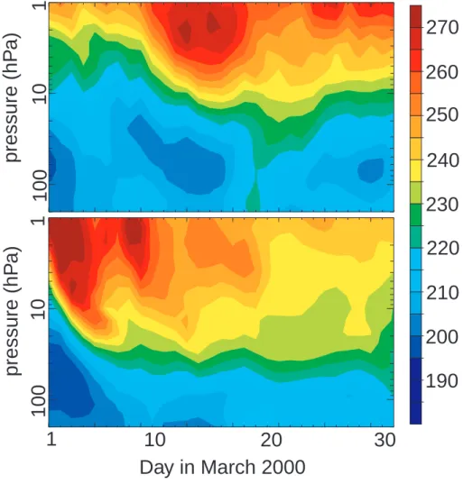
The main discrepancies are related to differences in the timing of sudden Arctic stratospheric warmings. For instance, the evolution of temperatures in 1999/2000 at 70 hPa is captured quite well. In the upper stratosphere, however, MAECHAM5/MESSy shows a strong major warming in early March 2000, after which the vortex does not fully recover (Fig. 4). The ECMWF analyses indeed show a warming about 10 days

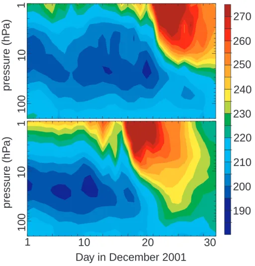
15

later, but subsequently the vortex recovers, particularly in the lower stratosphere. Fig-ure 5 shows that a similar ∼5 day advance of the warming occurs for December 2001, being a major event as discussed by Naujokat et al. (2002). In some other cases how-ever, the model captures the evolution of Arctic temperatures very well. For instance, in 2000/2001 the model exhibits a comparably disturbed vortex as in the analyses

af-20

ter late January, and then shows an analogous recovery around 20 February, with persistent cold temperatures well into March and April. Similarly good simulations are obtained in the Southern Hemisphere, for instance for September 2002, which includes the unique 2002 Antarctic vortex split (shown in Fig. 6).

The model thus has a mixed degree of success in capturing specific Arctic

sud-25

den stratospheric warmings, especially their timing, reflecting the fact that such events are driven by tropospheric waves as well as internal middle atmospheric dynamics (and their mutual interaction). In any case, the nudging clearly helps generating many characteristics of the overall temperature evolution during Arctic stratospheric winters.

(14)

ACPD

Full Screen / Esc

EGU Figure 7 present the same results as in the bottom panels of Figs. 1 and 3, but now

from a run without tropospheric nudging (except in the first four months). Note that this run did include the observed sea surface temperatures, as well as the equatorial QBO nudging. A comparison with Figs. 1 and 3 clearly shows that in both hemispheres, the nudged run provides a much closer match to the observed evolution of the

strato-5

spheric winters, even though in the Arctic the timing of specific stratospheric warmings is not simulated very well.

4.2. Midlatitudes

At midlatitudes (60, 50 and 40◦ north and south), the mean annual cycle as well as the seasonal and interannual variability in monthly mean temperatures are very well

10

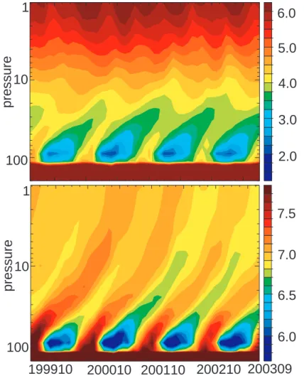
captured. At 70, 50, and 30 hPa, the model exhibits a small summer cold bias (up to about 2 K) similar to that at the poles. At 10 hPa however, the model shows a significant winter warm bias of several degrees K relative to the ECMWF analyses, particularly in the Southern Hemisphere. As an example, Fig. 8 shows the temperatures at 50◦S at 10 and 70 hPa.

15

4.3. Subtropics and tropics

We found that in the northern subtropical lower stratosphere (20◦N, 70 hPa and 50 hPa) the annual cycle in temperature of MAECHAM5/MESSy is smaller than of ECMWF; our model shows no or only a small cold bias in summer, but a substantial one in winter, up to about 5◦. This seasonal temperature bias is restricted to the outer reaches of the

20

domain of the QBO nudging (which tapers off between 10 and 20◦ North and South), and does not occur in a run without QBO nudging. It is caused by the uniform zonal winds used by the QBO nudging domain, which do not include the annual cycle in zonal wind at the subtropics. Sensitivity runs with more limited QBO nudging domains suggest that in future simulations the QBO nudging should be limited to to a somewhat

25

(15)

ACPD

Full Screen / Esc

EGU At all locations apart from the subtropics (discussed above), the fit between

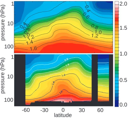
MAECHAM5/MESSy and ECMWF is improved for the run with QBO nudging. Not only, as expected, at the equator (where the QBO nudging is strongest), but also at midlatitudes and at the poles (although the effects there are smaller). A comparison between equatorial temperatures at 10 hPa for the runs with and without QBO nudging

5

(Fig. 9) indicates that the QBO forcing substantially improves the results; the run with-out QBO nudging clearly shows a bias that varies in parallel with the QBO cycle. Note also that the temporal tendency of the interannual variability is generally well captured, however, our model is often a few degrees colder than indicated by the ECMWF analy-ses. At 70 hPa, it is highest in the northern summer and very small in winter; at higher

10

altitudes, it is more constant through the seasons.

5. Results: methane and water vapor

We have also evaluated stratospheric methane and water vapor distributions (from the MESSy submodel H2O) to assess tracer transport throughout our four-year simula-tions. Unfortunately, there is no equivalent (in terms of coverage and resolution) of the

15

ECMWF analyzed temperatures for long-lived tracers, so we had to rely on less com-prehensive comparison methods. Firstly, we have compared “snapshots” of HALOE observations, both on individual days and during one HALOE sweep (which provides a zonal mean latitude-altitude perspective). Secondly, we have compared the time evo-lution of modeled methane and water vapor concentrations at particular altitudes and

20

latitudes with HALOE measurements taken around those locations.

5.1. Arctic and Antarctic methane

As in the simulations of Van Aalst et al. (submitted, 2004b)1, we obtained an excellent representation of the major warming and the split vortex in September 2002. Later in Antarctic winters, the model also captures specific details of the vortex evolution. As

(16)

ACPD

Full Screen / Esc

EGU an example, Fig. 10 shows methane concentrations at 74◦S on 3 November 2000 in

our MAECHAM5/MESSy simulations and as observed by HALOE (the HALOE image is composed of 15 vertical profiles observed over the course of the day). The model clearly reproduces the location of the vortex, and the edges of the vortex are su ffi-ciently sharp. Within the vortex, however, the model generally overestimates methane

5

concentrations below about 30 hPa. The tropopause transport barrier seems too be too high, and the vertical gradient too weak. It should be noted, however, that the ac-curacy of the HALOE data around the tropopause is relatively low. In the midlatitudes (roughly between 120 and 360◦) the simulated concentrations in the upper stratosphere are quite realistic; in the lower stratosphere however, the vertical gradients seem too

10

weak, resulting in an underestimate of methane between about 20 and 5–10 hPa, and an overestimate from the tropopause to about 50 hPa.

We obtained similar results for the Northern Hemisphere, to the extent that the com-parisons are unaffected by the different occurrence of stratospheric warmings, as dis-cussed above. For instance, for the 1999/2000 winter, the evolution of the late winter

15

vortex was quite different than in reality, so that a comparison with features in March would be meaningless. A slightly earlier comparison with the HALOE profiles on 20 February however (Fig. 11), shows that the model does simulate the vortex edge at around 300◦longitude. As in the Southern Hemisphere however, the methane concen-trations in the modeled vortex fragment below about 40 hPa are not sufficiently low. In

20

addition, contrary to the observations, the model also simulates a second feature in the upper stratosphere (at about 50◦longitude).

The transport deficiencies in the lower polar stratosphere are also illustrated by our longitudinal model-HALOE comparisons at 70◦N, shown in Fig. 12 (with decreasing mixing ratios on the vertical axis, so that the lines are represented in the order of their

25

altitude. This figure shows monthly and zonal mean model data (solid lines), and daily mean HALOE data (marks) from all days in our four-year run when the mean latitude of the HALOE observations were within a 3◦ window around 70◦N (if more than one daily mean latitude during one pass fell in the range, we took the one closest to the

(17)

ACPD

Full Screen / Esc

EGU target latitude). Note that this method introduces two comparison problems. Firstly,

MAECHAM5/MESSy profiles are consistently collected at a single latitude whereas the average latitude of the HALOE profiles varies. Furthermore, the HALOE data for a particular day do not originate in that average latitude, but are collected at different times and at slightly different latitudes (the range on one day can be up to about 8◦

5

halfway the latitude sweep at lower latitudes, less towards the turnaround points at higher latitudes). The variability induced by this sampling method is often too high to be able to assess the model’s ability to generate interannual variability in tracer trans-port. Finally, towards the poles, the coverage of the HALOE measurements diminishes, particularly during polar winters.

10

At 70◦N, the model reproduces the rise in lower stratospheric concentrations when the polar vortex disintegrates in spring (after light returns – when HALOE can perform measurements). The quantitative match of the methane concentrations is very good at 10 hPa (and higher), but rather poor in the lower stratosphere, consistent with the results of the snapshots at 3 November and 20 February 2000 (Figs. 10 and 11). The

15

reason is a too high tropopause and a too weak vertical gradient up to about 40 hPa. This lack of isolation of the lower vortex also results in an underestimate of descent rates in the vortex (as estimated on the basis of tracer concentrations through the win-ter). Van Aalst et al. (2004a) identified a similar lack of descent in the lower part of the Arctic vortex in fully nudged simulations of the 1999/2000 winter (with MAECHAM4

20

and the semi-Lagrangian advection scheme). We repeated the tracer descent calcu-lations from that analysis with our current model data, and found very similar results: a good match with observations (Greenblatt et al., 2002) of descent starting at po-tential temperatures around 550 and 500 K (about 30–40 hPa) in early December, but an underestimate of descent starting around 450 and 400 K (about 50–100 hPa). This

25

problem may substantially affect both transport and chemistry in the lower polar vortex, and requires careful attention in the analysis of model data from that region.

In the Antarctic, HALOE observations regularly capture vortex features during Oc-tober, November and December when the orbit crosses 70◦ south. Given the large

(18)

ACPD

Full Screen / Esc

EGU differences in concentration inside and outside the vortex, this introduces too much

variability to make a useful comparison like the one in Fig. 12 at 70◦N (in this case, the only meaningful comparison between MAECHAM5/MESSy and HALOE is to take individual days and latitudes, as in the snapshots discussed above). Nevertheless, the overall impression of such comparisons is the same as in the Northern Hemisphere:

5

too high methane values in the lowermost stratosphere, and suppressed descent, ap-parently due to too strong vertical mixing.

5.2. Global methane

The equatorial region, where trace gases like methane enter the stratosphere and are transported upwards, plays a crucial role in middle atmospheric transport.

10

Figure 13 shows a comparison between modeled monthly mean CH₄ data and HALOE observations at the equator. After substantial differences in the first few months (caused by the initialization, which was based upon 3 years of HALOE data for April/May, not specifically for 1 May 1999), the match is generally very good. The model also captures the modulation of the methane concentrations by the QBO,

al-15

though it is slightly weaker than in the HALOE measurements (for instance at 10 hPa). As expected, the run without QBO nudging did not show this modulation, resulting in a substantially poorer match with the HALOE measurements (here, and in other parts of the stratosphere).

Figure 14 shows a comparison of modeled zonal mean methane concentrations on

20

23 August 2000, compared to observations from 40-day HALOE sweeps around that day. It shows a general agreement in concentrations, as well as a good reproduction of the instantaneous shape of the concentration profiles (similar model-HALOE agree-ment is obtained at other days throughout the run). However, methane concentrations in the lower stratosphere at southern midlatitudes are too high, and the vertical gradient

25

at the top of the “shoulder” is too weak. These problems also appear in detailed com-parisons. In northern midlatitudes and in the subtropics, the HALOE measurements are generally in good agreement with the model’s monthly mean methane

(19)

concentra-ACPD

Full Screen / Esc

EGU tions, and some, but not all specific features of the interannual variability are captured

by the model (e.g. Fig. 15). At southern midlatitudes however, the vertical gradient is too smooth, and the model does not capture the annual shifts in methane concen-trations in the mid-stratosphere (again, because the weak gradients at the top of the midlatitude shoulder).

5

5.3. Water vapor

Given the realistic methane concentrations in most of the stratosphere, the model also simulates an accurate chemical source for water vapor. However, middle atmospheric water vapor concentrations also depend on the seasonal water vapor cycle in the air that enters the stratosphere. The general pattern of the upward propagation of this

10

seasonal cycle, the tropical tape recorder (Mote et al., 1996), is well modeled, as shown in Fig. 16.

The model also generates realistic stratospheric water vapor distributions, although it fails to capture several important details in the lower stratosphere. This can be seen in Fig. 17, which shows the same model-HALOE comparisons as in Fig. 14 (zonal mean,

15

latitude-altitude) and Fig. 10 (longitude-altitude), but now for water vapor. The model does not simulate the lowest concentrations in the lower equatorial stratosphere, and falls short with respect to the minimum of the previous year around 24 hPa, clearly visible in HALOE data. In midlatitudes, the vertical gradient above the water vapor minimum in the lower stratosphere is too weak, while concentrations in the lowermost

20

stratosphere too high. At the poles, a similar transport problem appears as in methane, with substantially too high water vapor in the lowermost stratosphere. On 3 November 2000, the overall shape of the vortex feature and the location of minima and maxima are well modeled, but the model simulates a too high tropopause and fails to capture the deepest minima in the lower stratosphere. In midlatitude air, the same smoothed

25

(20)

ACPD

Full Screen / Esc

EGU

6. Discussion

We found that MAECHAM5/MESSy with nudging up to 113 hPa simulates the main features of the large-scale circulation in the middle atmosphere, including its seasonal and interannual variability. However, specific aspects of polar winters, particularly the timing of sudden stratospheric warmings in the Northern Hemisphere, are not always

5

accurately reproduced. This mainly reflects the more dynamically active circumstances in the Northern Hemisphere, and may partly be related to the model’s relatively coarse vertical resolution, which is known to be insufficient to reproduce certain aspects of wave-driven dynamics (including the QBO).

MAECHAM5/MESSy generally simulates realistic temperatures, including the

tem-10

perature minima in the Antarctic winter. A few biases remain, including a cold bias throughout the lower stratosphere (consistent with, e.g. the model intercomparison by Pawson et al., 2000). Sensitivity runs without tropospheric nudging (but with correct sea surface temperatures and the QBO forcing) showed that the tropospheric nudging is not for the cause of these biases in the model, and it does not create other ones.

15

This finding confirms that our nudging settings and normal mode filtering prevent the nudging from generating spurious gravity waves that might affect middle atmospheric dynamics.

The tracer distributions are generally realistic except for too weak gradients at mid-latitudes, and, particularly, a too high tropopause and too weak vertical gradient in the

20

polar lower stratosphere, which also results in an underestimate of descent rates in the polar vortex. Similar problems with tracer descent in the vortex were identified in CTM studies (though not affected by a tropopause bias). For instance, Plumb et al. (2002) identified excessive horizontal mixing inside the vortex and between vor-tex and extra-vorvor-tex air in CTM studies for the 1999/2000 winter. In an analysis that

25

separated horizontal and vertical tracer exchange, Considine et al. (2003) found that their CTM exhibited compensating errors; too vigorous descent in the meteorological input data was counterbalanced by an overestimate of horizontal mixing. Using the

(21)

ACPD

Full Screen / Esc

EGU TM5 zoom model, Bregman (personal communication) show that the problems with

tracer descent in the 1999/2000 Arctic vortex that were identified by Van den Broek et al. (2003) were partly related to the reduced grid employed in earlier versions of that CTM (a problem that does not apply to MAECHAM5/MESSy). However, they also showed that substantial improvements were achieved with the second order

advec-5

tion scheme developed by Prather (1986) than with the more diffuse Slopes advection scheme (Russell and Lerner, 1981), and that a similar improvement resulted from a substantially higher horizontal resolution (1×1 instead of 2×3◦). Unfortunately, both solutions (either the second order advection or the higher resolution) come at a high price in terms of computing resources.

10

In our simulations, we also obtained a slight improvement in runs at higher horizontal resolution (T63 instead of T42). If horizontal mixing would be the primary cause of the relatively high methane concentrations in the lower vortex, however, we would also expect a more diffusive tracer advection scheme to perform worse than the current FFSL scheme, which did not appear to be the case. Instead, sensitivity tests with the

15

more diffuse semi-Lagrangian transport scheme produced better results in the lower vortex, although the best results were achieved with the SPITFIRE advection scheme, which is least diffusive of the three. We note however, that the SPITFIRE scheme underestimates upward transport at the equator (as noted by Steil et al., 2003) while the semi-Lagrangian scheme does not capture sharp gradients, for instance at the

20

subtropical barrier and at edge of the vortex, so that all three schemes have significant drawbacks. In addition, even the (least diffusive) SPITFIRE scheme still overestimates methane in the lower stratospheric polar vortex. We suspect that the vertical resolution may be an important factor, not the least because a higher vertical resolution would likely also result in a lower tropopause (as in the runs by Roeckner et al. (2004) with

25

the standard ECHAM5 up to 10 hPa). Therefore, it would be interesting to repeat the simulations with the MAECHAM5 version with higher vertical resolution employed by Giorgetta et al. (2002), which reproduces a QBO without assimilation (although a weak nudging might still be needed to keep the model’s internal QBO synchronized with the

(22)

ACPD

Full Screen / Esc

EGU observations), and should also perform better in simulating wave phenomena in polar

winters. Bregman (personal communication) found that in runs with the TM5 CTM at very high resolution (up to one by one degree), the vertical resolution did not have much influence on tracer transport below 10 hPa. We emphasize however, that regardless of the model resolution, CTM winds are taken from the high-resolution ECMWF analyses.

5

In the case of our MAECHAM5/MESSy runs, the vertical resolution also affects the model dynamics, including the location of the tropopause.

Finally, we note that the advection in MAECHAM5/MESSy suffers from a mass imbal-ance, caused by a mismatch between the mass fluxes and surface pressure tendencies (which are calculated independently), and the transformation of spectral divergence,

10

vorticity and surface pressure to three-dimensional winds for trace gas advection at the Gaussian grid (see J ¨ockel et al., 2001; Bregman et al., 2003). Sensitivity tests with an iterative correction of this mismatch showed that this is not the primary cause of the transport problems in the polar lower stratosphere (although it did create significant changes at some other locations in the stratosphere). Ideally, GCMs should provide

15

a consistent representation of dynamics and transport on one grid. Yet another way to improve stratospheric transport would be to employ an isentropic vertical coordi-nate system (Mahowald et al., 2002), but this would require equally dramatic model changes, unsuited for coupled stratosphere-troposphere simulations.

7. Conclusions

20

We have performed a multi-year integration with the MAECHAM5/MESSy middle at-mosphere GCM, while nudging the dynamics in the free troposphere (below 113 hPa) towards ECMWF meteorological analyses. In addition, we force a realistic QBO by as-similation of equatorial zonal wind observations. We show that this model setup allows simulations of many synoptic features of the middle atmospheric dynamics. In

Antarc-25

tic winters, the model generally reproduces the observed stratospheric meteorology very closely. In the Arctic region, however, the model does not always capture the

(23)

ACPD

Full Screen / Esc

EGU timing and evolution of sudden stratospheric warmings, reflecting the more dynamic

stratosphere in Northern compared to Southern winters. We conclude that this setup provides good opportunities for further studies with coupled-climate simulations of the middle atmosphere, for instance for the period covered by the ERA-40 reanalysis, but that comparisons with measurements on individual days in the Arctic must be

inter-5

preted with care.

Comparing the modeled temperatures to those in the ECMWF analyses, we found that the model exhibits a slight cold bias in the lower stratosphere, particularly at mid-latitudes, and at the poles during summer. Arctic and Antarctic winter temperatures are simulated very well, including the extent of low temperatures needed for the formation

10

of PSCs. A warm bias in polar spring will likely be reduced in simulations with coupled chemistry instead of the current ozone climatology.

Stratospheric methane and water vapor concentrations generally compare well to HALOE observations, except in the equatorial lower stratosphere, where the water vapor minimum is not well simulated, and in the polar lower stratosphere, where the

15

model simulates a too high tropopause and too weak vertical gradients. The latter transport problem may provide limitations for coupled chemistry-climate studies of polar ozone loss. The choice of the advection scheme and the horizontal resolution both play a role, but the problem will probably be reduced most effectively by enhancing the vertical resolution. Such a higher resolution could also produce an explicit QBO

20

(i.e. without QBO nudging) and might improve the simulation of dynamic troposphere-stratosphere coupling in the Arctic region.

At the current vertical resolution, we find that the assimilation of observed strato-spheric equatorial zonal winds to force a realistic QBO improves our results: it not only results in a better match of equatorial winds and temperatures with the ECMWF

25

analyses, but also helps to simulate QBO-like features in the global tracer fields, and improves the temperature fields at the poles. However, the extent of the QBO nudging domain should be chosen carefully to avoid suppression of the subtropical annual cycle in winds and temperatures.

(24)

ACPD

Full Screen / Esc

EGU

Acknowledgements. We thank the HALOE team at NASA/Langley for making their data avail-able on the internet. The computer simulations were performed at the Computing Centre of the Max Planck Society in Garching (RZG), and at the Dutch computing center SARA (with support from the Netherlands Computing Facilities Foundation NCF).

References

5

Austin, J.: A three-dimensional coupled chemistry-climate model simulation of past strato-spheric trends, J. Atmos. Sci., 59, 218–232, 2002.

Austin, J., Shepherd, T. G., Schnadt, C., Rozanov, E., Pitari, G., Pawson, S., Newman, P., Nagashima, T., Manzini, E., Dameris, M., Br ¨uhl, C., and Beagley, S. R.: Uncertainties and assessments of chemistry-climate models of the stratosphere, Atmos. Chem. Phys., 3, 1–27,

10

2003,

SRef-ID: 1680-7324/acp/2003-3-1.

Baldwin, M. P., Gray, L. J., Dunkerton, T. J., Hamilton, K., Haynes, P. H., Randel, W. J., Holton, J. R., Alexander, M. J., Hirota, I., Horinouchi, T., Jones, D. B. A., Kinnersley, J. S., Marquardt, C., Sato, K., and Takahashi, M.: The quasi-biennial oscillation, Rev. Geophys., 39, 179–229,

15

2001.

Bregman, A., Segers, A., Krol, M., Meijer, E., and van Velthoven, P.: On the use of mass-conserving wind fields in chemistry-transport models, Atmos. Chem. Phys., 3, 447–457, 2003,

SRef-ID: 1680-7324/acp/2003-3-447.

20

Considine, D. B., Kawa, S. R., Schoeberl, M. R., and Douglass, A. R.: N₂O and NO_y observa-tions in the 1999/2000 Arctic Polar Vortex: Implicaobserva-tions for transport processes in a CTM, J. Geophys. Res., 108(D5), 4170, doi:10.1029/2002JD002525, 2003.

Fortuin, J. P. F. and Kelder, H.: An ozone climatology based on ozonesonde and satellite mea-surements, J. Geophys. Res., 103(D24), 31 709–31 734, 1998.

25

Fritts, D. C. and Alexander, M. J.: Gravity wave dynamics and effects in the middle atmosphere, Rev. Geophys., 41(1), art. no. 1003, doi:10.1029/2001RG000106, 2003.

Giorgetta, M. A. and Bengtsson, L.: The potential role of the quasi-biennial oscillation in the stratosphere-troposphere exchange as found in water vapour in general circulation model experiments, J. Geophys. Res., 104, 6003–6019, 1999.

(25)

ACPD

Full Screen / Esc

EGU

Giorgetta, M. A., Manzini, E., and Roeckner, E.: Forcing of the quasi-biennial oscilla-tion from a broad spectrum of atmospheric waves, Geophys. Res. Lett., 29(D8), 1245, doi:10.1029/2002GL014756, 2002.

Greenblatt, J. B., Jost, J. J., Loewenstein, M., Podolske, J. R., Hurst, D. F., Elkins, J. W., Schauffler, S. M., Atlas, E. L., Herman, R. L., Webster, C. R., Bui, T. P., Moore, F. L., Ray,

5

E. A., Oltmans, S., Vomel, H., Blavier, J.-F., Sen, B., Stachnik, R. A., Toon, G. C., Engle, A., Muller, M., Schmidt, U., Bremer, H., Pierce, R. B., Sinnhuber, B.-M., Chipperfield, M., and Lefevre, F.: Tracer-based determination of vortex descent in the 1999–2000 Arctic winter, J. Geophys. Res., 107(D20), 8279, doi:10.1029/2001JD000937, 2002.

Guldberg, A. and Kaas, E.: Danish Meteorological Institute Contribution to the Final Report,

10

in: Project On Tendency Evaluations Using New Techniques to Improve Atmospheric Long-term Simulations (POTENTIALS) – Final Report, edited by: Kaas, E., Danish Meteorological Institute (DMI), Copenhagen, Denmark, 2000.

Hamilton, K.: Effects of an imposed quasi-biennial oscillation in a comprehensive troposphere-stratosphere-mesosphere general circulation model, J. Atmos. Sci., 55(14), 2393–2418,

15

1998.

Harries III, J. E., Tuck, A. F., Gordley, L. L., Purcell, P., Stone, K., Bevilacqua, R. M., Gun-son, M., Nedoluha, G., and Traub, W. A.: Validation of measurements of water vapor from the Halogen Occultation Experiment (HALOE), J. Geophys. Res., 101(D6), 10 205–10 216, doi:10.1029/95JD02933, 1996.

20

Hertzog, A., Basdevant, C., Vial, F., and Mechoso, C. R.: Some results on the accuracy of stratospheric analyses in the Northern Hemisphere inferred from long-duration balloon flights, Q. J. R. Meteorol. Soc., 130, 607–626, 2004.

Jeuken, A. B. M., Siegmund, P. C., Heijboer, L. C., Feichter, J., and Bengtson, L.: On the potential of assimilating meteorological analysis in a climate model for the purpose of model

25

validation, J. Geophys. Res., 101, 16 939–16 950, 1996.

J ¨ockel, P., von Kuhlmann, R., Lawrence, M. G., Steil, B., Brenninkmeijer, C. A. M., Crutzen, P. J., Rasch, P. J., and Eaton, B.: On a fundamental problem in implementing flux-form advection schemes for tracer transport in 3-dimensional general circulation and chemistry transport models, Q. J. R. Meteorol. Soc., 127A, 1035–1052, 2001.

30

J ¨ockel, P., Sander, R., and Lelieveld, J.: Technical Note: The Modular Earth Submodel System (MESSy) – a new approach towards Earth System Modeling, Atmos. Chem. Phys., 5, 433– 444, 2005,

(26)

ACPD

Full Screen / Esc

EGU

SRef-ID: 1680-7324/acp/2005-5-433.

Knudsen B. M.: On the accuracy of analysed low temperatures in the stratosphere, Atmos. Chem. Phys., 3, 1759–1768, 2003,

SRef-ID: 1680-7324/acp/2003-3-1759.

Knudsen, B. M., Pommereau, J.-P., Garnier, A., Nunes-Pnharanda, M., Denis, L., Newman, P.,

5

Letrenne, G., and Durand, M.: Accuracy of analyzed stratospheric temperatures in the winter Arctic vortex from infrared Montgolfier long-duration balloon flights, 2. Results, J. Geophys. Res., 107(D20), doi:10.1029/2001JD001329, 2002.

Lin, S. J. and Rood, R. B.: Multi-dimensional flux-form semi-Lagrangian transport schemes, Mon. Wea. Rev., 124, 2046–2070, 1996.

10

Lohmann, U. and Roeckner, E.: Design and performance of a new cloud microphysics scheme developed for the ECHAM4 general circulation model, Clim. Dyn., 12, 557–572, 1996. Mahowald, N. M., Plumb, R. A., Rasch, P. J., del Corral, J., Sassi, F., and Heres, W.:

Stratospheric transport in a 3-dimensional isentropic coordinate model, J. Geophys. Res, 107(D15), doi:10.1029/2001JD1313, 2002.

15

Manney, G. L., Sabutis, J. L., Pawson, S., Santee, M. L., Naujokat, B., Swinbank, R., Gelman, M. E., and Ebisuzaki, W.: Lower stratospheric temperature differences between meteoro-logical analyses in two cold Arctic winters and their impact on polar processing studies, J. Geophys. Res., 108(D5), 8328, doi:10.1029/2001JD001149, 2003.

Manzini, E. and McFarlane, N. A.: The effect of varying the source spectrum of a gravity wave

20

parameterization in a middle atmosphere general circulation model, J. Geophys. Res., 103, 31 523–31 539, 1998.

Manzini, E., McFarlane, N. A., and McLandress, C.: Impact of the Doppler spread parameter-ization on the simulation of the middle atmosphere circulation using the MA/ECHAM4 gen-eral circulation model, J. Geophys. Res., 102(D22), 25 751–25 762, doi:10.1029/97JD01096,

25

1997.

Manzini, E., Steil, B., Br ¨uhl, C., Giorgetta, M. A., and Kr ¨uger, K.: A new interactive chemistry-climate model: 2. Sensitivity of the middle atmosphere to ozone depletion and increase in greenhouse gases and implications for recent stratospheric cooling, J. Geophys. Res., 108(D14), 4429, doi:10.1029/2002JD002977, 2003.

30

Marquardt, C. and Naujokat, B.: An update of the equatorial QBO and its variability, 1st SPARC General Assembly, Melbourne Australia, WMO/TD-No. 814, 1, 87–90, 1997.

(27)

ACPD

Full Screen / Esc

EGU

transfer scheme, RRTM, on the ECMWF model climate and 10-day forecasts, Technical Memorandum 252, ECMWF, Reading, UK, 1998.

Mote, P. W., Rosenlof, K. H., McIntyre, M. E, Carr, E. S., Gille, J. C., Holton, J. R., Kinnersley, J. S., Pumphrey, H. C., Russell III, J. M., and Waters, J. W.: An atmospheric tape recorder: the imprint of tropical tropopause temperatures on stratospheric water vapor, J. Geophys. Res.,

5

101, 3989–4006, 1996.

Naujokat, B.: An update of the observed quasi-biennial oscillation of the stratospheric winds over the tropics, J. Atmos. Sci., 43, 1873–1877, 1986.

Naujokat, B., Kr ¨uger, K., Matthes, K., Hoffmann, J., Kunze, M., and Labitzke, K.: The early major warming in December 2001 – exceptional?, Geophys. Res. Lett., 29(21), 2023,

10

doi:10.1029/2002GL015316, 2002.

Park, J. H., Russell III, J. M., Gordley, L. L., Drayson, S. R., Benner, C. D., McInerney, J., Gunson, M. R., Toon, G. G., Sen, B., Blavier, J.-F., Webster, C. R., Zipf, E. C., Erdman, P., Schmidt, U., and Schiller, C.: Validation of Halogen Occultation Experiment CH4 Measure-ments from the UARS, J. Geophys. Res., 101, 10 183–10 203, 1996.

15

Pawson, S., Kodera, K., Hamilton, K., Shepherd, T. G., Beagley, S. R., Boville, B. A., Farrara, J. D., Fairlie, T. D. A., Kitoh, A., Lahoz, W. A., Langematz, U., Manzini, E., Rind, D. H., Scaife, A., Shibata, K., Simon, P., Swinbank, R., Takacs, L., Wilson, R. J., Al-Saadi, J. A., Amodei, M., Chiba, M., Coy, L., deGrandpr ´e, J., Eckman, R. S., Fiorino, M., Grose, W. L., Koide, H., Koshyk, J. N., Li, D., Lerner, J., Mahlman, J. D., McFarlane, N. A., Mechoso, C. R., Molod,

20

A., O’Neill, A., Pierce, R. B., Randel, W. J., Rood, R. B., and Wu, F.: The GCM-Reality Intercomparison Project for SPARC (GRIPS): Scientific Issues and Initial Results, Bull. Am. Meteorol. Soc., 81, 781–796, 2000.

Pommereau, J.-P., Garnier, A., Knudsen, B. M., Letrenne, G., Durand, M., Nunes-Pinharanda, M., Denis, L., Vial, F., Hertzog, A., and Cairo, F.: Accuracy of analyzed stratospheric

tem-25

peratures in the winter arctic vortex from infrared Montgolfier long duration balloon flights, 1, Measurements, J. Geophys. Res., 107(D20), doi:10.1029/2001JD001379, 2002.

Prather, M.: Numerical advection by conservation of second-order moments, J. Geophys. Res., 91, 6671–6681, 1986.

Rasch, P. J. and Lawrence, M.: Recent Developments in Transport Methods at NCAR, in:

30

MPI Workshop on conservative transport schemes, MPI-report 265, Max-Planck-Institute for Meteorology, Hamburg, Germany, 1998.

(28)

ACPD

Full Screen / Esc

EGU

transport, SIAM, J. Sci. Stat. Comput., 11, 656–687, 1990.

Rasch, P. J., Boville, B. A., and Brasseur, G. P.: A threedimensional general circulation model with coupled chemistry for the middle atmosphere, J. Geophys. Res., 100, 9041–9071, 1995.

Roeckner, E., Arpe, K., Bengtsson, L., Christoph, M., Claussen, M., D ¨umenil, L., Esch, M.,

5

Giorgetta, M., Schlese, U., and Schulzweida, U.: The atmospheric general circulation model ECHAM4: Model description and simulation of present-day climate, MPI Report 218, Ham-burg, Germany, 1996.

Roeckner, E., B ¨auml, G., Bonaventura, L., Brokopf, R., Esch, M., Giorgetta, M., Hagemann, S., Kirchner, I., Kornblueh, L., Manzini, E., Rhodin, A., Schlese, U., Schulzweida, U., and

Tomp-10

kins, A.: The atmospheric general circulation model ECHAM 5. PART I: Model description, MPI-Report 349, Hamburg, Germany, 2003.

Roeckner, E., Brokopf, R., Esch, M., Giorgetta, M., Hagemann, S., Kornblueh, L., Manzini, E., Schlese, U., and Schulzweida, U.: The atmospheric general circulation model ECHAM 5, PART II: Sensitivity of Simulated Climate to Horizontal and Vertical Resolution, MPI-Report

15

354, Hamburg, Germany, 2004.

Russell, G. M. and Lerner, J. A.: A new finite-differencing scheme for the tracer transport equation, J. Appl. Meteorol., 20, 1483–1498, 1993.

Russell III, J. M., Gordley, L. L., Park, J. H., Drayson, S. R., Hesketh, D. H., Cicerone, R. J., Tuck, A. F., Frederick, J. E., Harries, J. E., and Crutzen, P. J.: The Halogen Occultation

20

Experiment, J. Geophys. Res., 98, 10 777–10 797, 1993.

Schulz, J.-P., D ¨umenil, L., and Polcher, J.: On the land surface-atmosphere coupling and its impact in a single-column atmospheric model, J. Appl. Meteorol., 40, 642–663, 2001. Simmons, A. J. and Gibson, J. K.: The ERA40 Project Plan, ERA40 Project Report Series No.

1, ECMWF, Reading, UK, 2000.

25

Simmons, A. J., Burridge, D. M., Jarraud, M., Girard, C., and Wergen, W.: The ECMWF medium-range prediction model: Development of the numerical formulations and the impact of increased resolution, Meteorol. Atmos. Phys., 40, 28–60, 1989.

Simmons, A., Hortal, M., Kelly, G., McNally, A., Untch, A., and Uppala, S.: ECMWF analyses and forecasts of stratospheric winter polar vortex break-up: September 2002 in the Southern

30

Hemisphere and related events, J. Atmos. Sci., in press, 2005.

Steil, B., Br ¨uhl, C., Manzini, E., Crutzen, P. J., Lelieveld, J., Rasch, P. J., Roeckner, E., and Kr ¨uger, K.: A new interactive chemistry climate model, I: Present day climatology and

(29)

inter-ACPD

Full Screen / Esc

EGU

annual variability of the middle atmosphere using the model and 9 years of HALOE/UARS data, J. Geophys. Res., 108(D9), 4290, doi:10.1029/2002JD002971, 2003.

Van Aalst, M. K., van den Broek, M. M. P., Bregman, A., Br ¨uhl, C., Steil, B., Toon, G. C., Garcelon, S., Hansford, G. M., Jones, R. L., Gardiner, T. D., Roelofs, G. J., Lelieveld, J., and Crutzen, P. J.: Trace gas transport in the 1999/2000 Arctic winter; comparison of nudged

5

GCM runs with observations, Atmos. Chem. Phys., 4, 81–93, 2004a, SRef-ID: 1680-7324/acp/2004-4-81.

Van den Broek, M. M. P., van Aalst, M. K., Bregman, A., Krol, M., Lelieveld, J., Toon, G. C., Garcelon, S., Hansford, G. M., Jones, R. L., and Gardiner, T. D.: The impact of model grid zooming on tracer transport in the 1999/2000 Arctic polar vortex, Atmos. Chem. Phys., 3,

10

1833–1847, 2003,

(30)

ACPD

Full Screen / Esc

EGU Table 1. Relative difference between MAECHAM5/MESSy and ECMWF in area with

tempera-tures lower than 190 K during the month of August.

54 hPa 70 hPa 2000 12% 9% 2001 22% 48% 2002 8% 9% 2003 10% 0%

(31)

ACPD

Full Screen / Esc

EGU Fig. 1. Monthly temperatures (K) at 80◦S, 10 hPa (top) and 70 hPa (bottom), for

MAECHAM5/MESSy (red) and ECMWF (blue). Thick solid lines represent the mean, colored dashed lines the 33 and 66 percentiles, and black dashed lines the minimum and maximum values.

(32)