Identification of the low-altitude cusp by Super Dual Auroral Radar Network radars: A physical explanation for the empirically derived signature

HAL Id: insu-03002185

https://hal-insu.archives-ouvertes.fr/insu-03002185

Submitted on 12 Nov 2020

HAL is a multi-disciplinary open access

archive for the deposit and dissemination of

sci-entific research documents, whether they are

pub-lished or not. The documents may come from

teaching and research institutions in France or

abroad, or from public or private research centers.

L’archive ouverte pluridisciplinaire HAL, est

destinée au dépôt et à la diffusion de documents

scientifiques de niveau recherche, publiés ou non,

émanant des établissements d’enseignement et de

recherche français ou étrangers, des laboratoires

publics ou privés.

Identification of the low-altitude cusp by Super Dual

Auroral Radar Network radars: A physical explanation

for the empirically derived signature

R. Andre, M. Pinnock, A.S. Rodger

To cite this version:

R. Andre, M. Pinnock, A.S. Rodger. Identification of the low-altitude cusp by Super Dual Auroral

Radar Network radars: A physical explanation for the empirically derived signature. Journal of

Geophysical Research Space Physics, American Geophysical Union/Wiley, 2000, 105 (A12), pp.81

-108. �10.1029/2000JA900071�. �insu-03002185�

JOURNAL OF GEOPHYSICAL RESEARCH, VOL. 105, NO. A12, PAGES 27,081-27,093, DECEMBER 1, 2000

Identification of the low-altitude cusp by Super Dual Auroral

Radar Network radars: A physical explanation for the

empirically derived signature

R. Andre,

t M. Pinnock,

and A. S. Rodger

British Antarctic Survey, Natural Environment Research Council, Cambridge, England

Abstract. The Super Dual Auroral Radar Network (SuperDARN) radars are proving to

be a very powerful experimental tool for exploring solar wind-magnetosphere-ionosphere

interactions. They measure the autocorrelation function (ACF) of the signal backscattered

from ionospheric

irregularities,

and they derive parameters

such

as the Doppler velocity

and the spectral

width. The associated

spectra

have a specific

behavior

inside the cusp, a

strong

temporal

and spatial

evolution

of the velocity and spectral

width, and a high value

of the spectral width. Until now, no studies have explained these characteristics, but they

are routinely used to detect the cusp in the radar data, for example, to estimate the location

of the open/closed

field line boundary.

Both satellite

and ground-based

magnetometer

data

from the cusp

region show

broadband

wave activity in the Pcl and Pc2 frequency

band. In

this study we evaluate how such wave activity modifies the radar's ACF, and we conclude

that it explains

the spectra

seen in the cusp. More specifically,

we find that (1) even a

monochromatic electric field variation can cause apparently turbulent behavior, including

wide spectral

widths and apparent

multiple components,

(2) even low-amplitude

waves

are capable

of causing

large spectral

widths,

if the frequency

is sufficiently

high, (3) for

a fixed low-amplitude

electric field variation

the measured

spectral

width increases

with

wave frequency,

displaying

a sharp

transition

from low to high spectral

width above an

onset

frequency,

and (4) the determination

of the background

velocity

field is not strongly

affected by such conditions. While the wave activity is shown to have a major impact on

the spectral

width, it is found that the radar does

accurately

represent

the large-scale

plasma

velocity.

1. Introduction

Identification of the ionospheric signature of the cusp is

important for many studies of solar wind-magnetosphere- ionosphere coupling processes. For example, the cusp signa- ture is a proxy for the open/closed field line boundary on the

dayside, and flow across this boundary is a measure of the

reconnection rate at the magnetopause [Baker et al., 1997]. Several techniques have been used for identifying the cusp at low altitudes, the most widely accepted being the signa- ture of cusp particle precipitation in polar-orbiting satellites such as Defense Meteorological Satellite Program (DMSP) [Newell and Meng, 1988], but ground-based magnetometer

signatures [Menk et al., 1992] have also been used. HF radar

data have been found to contain a distinctive signature of the

•Now at Laboratoire de Physique et Chimie de l'Environnement,

Centre National de la Recherche Scientifique, Orlrans, France.

Copyfight 2000 by the American Geophysical Union. Paper number 2000JA900071.

0148-0227/00/2000JA900071 $09.00

low-altitude cusp [e.g., Baker et al., 1995], but the physical explanation has remained elusive. It is the topic of this paper.

From the transmission of a multiple-pulse scheme the

Super Dual Auroral Radar Network (SuperDARN) radars

[Greenwald et al., 1995] measure the autocorrelation func-

tion (ACF) of the signal backscattered at several distances (range gates) from the radar by field-aligned electron con- centration irregularities. In each range gate, this ACF is routinely analyzed by a basic method (called FITACF) [Vil- lain et al., 1987; Baker et al., 1995, Appendix A] which ex- tracts the power, the line-of-sight Doppler velocity of the irregularities, and the spectral width. Baker et al. [1995]

have found that the ACFs recorded in the cusp have a very

particular behavior. They showed that the Doppler velocity

spectrum observed in the cusp, which was detected from the

particle characteristics [Newell and Meng, 1988] recorded by a DMSP satellite, presents several overlapping compo- nents from which a high spectral width value is determined. Although no studies have explained this behavior, the cusp could easily be identified in the radar data by a high and variable spectral width, and variable line-of-sight velocity

[Pinnock et al., 1995].

27,082 ANDRt2 ET AL.: LOW-ALTITUDE CUSP SEEN BY HF RADARS

Intense wave activity has been observed when satellites pass through the cusp [see, e.g., Maynard et al., 1991].

Matsuoka et al. [1993], and later Erlandson and Anderson

[1996], have clearly shown a step-like increase of wave ac- tivity in the frequency band 0.2-2.2 Hz with electric field

values of a few mV m -•, coincident with the equatorward

edge of the cusp particle precipitation. These waves appear to result from a superposition of an electrostatic noise and electromagnetic waves. On the ground the electromagnetic part of this wave activity in the Pc 1 and Pc2 wave band has been recorded by magnetometers, as shown, for example, by Menk et al. [1992] and Dyrud et al. [1997], although there is

some contradiction in these two studies as to the latitude at which the waves are observed.

In this paper we evaluate the effect of such a time-varying

electric field component on the determination of the radar ACF, and we extend the results recently published [Andrg et al., 1999]. In section 2 a detailed description of the wave activity as seen on board satellites and on the ground in the cusp region is given. The characteristics of the HF radar data obtained in the cusp are also discussed. Simulating the radar operating mode, section 3 shows that a monochromatic wave (Pc 1) of realistic amplitude for the cusp region can affect the radar signal processing such as to increase the radar spectral

width. This result is then extended to a more realistic wave

activity by considering the case of a narrow band wave. The sources of these waves in the magnetosphere are then dis- cussed, and we conclude that they can explain the high spec- tral width values observed in radar spectra from the morning sector and especially in the cusp.

2. Wave Observations in the Cusp

The low-altitude cusp has been defined from the particle data [Newell and Meng, 1988, p. 14550] as a "localized re- gion in which magnetosheath plasma entry is more direct." In this region the particles have to maintain their original (magnetosheath) spectral characteristics with a high num- ber flux. Newell and Meng [1988, 1989, 1992] and Newell et al. [1989] use a large number of DMSP satellite passes to derive a particle definition of the cusp and its statistical po- sition depending on the interplanetary magnetic field (IMF)

conditions.

Using the Dynamic Explorer 2 (DE 2) data, Curtis et al. [ 1982] and Maynard [ 1985] showed broadband electrostatic

step-like increase of the power spectrum, they found an in- crease of the electrostatic noise power, which limits their Pc 1 detection. Studying the magnetic component, they showed that the electric to magnetic field ratio strongly suggests an

Alfv6nic behavior of these waves.

At higher altitude, Matsuoka et al. [ 1991, 1993] observed a similar electromagnetic wave activity in the Exos-D satel- lite data, and they showed that the electric fluctuations in the cusp are more intense than those observed in the dayside au-

roral region. They showed a very good correlation between

the latitude of the increase of the power spectral density in the Pc 1-Pc2 frequency band and the increase of the magne- tosheath particle flux in the cusp. They also found that these fluctuations are consistent with an Alfv6n wave interpreta-

tion.

2.2. Magnetometer Data

By using several ground stations, Bolshakova et al. [1980]

found that the Pc 1-Pc2 occurrence is a maximum when the

equatorward edge of the cusp is close to a station. Later, Morris and Cole [1991] and especially Menk et al. [1992] separate these waves into several categories and found that

narrowband Pc 1-Pc2 waves are mostly observed a few de-

grees equatorward of the plasma sheet boundary layer in the

noon sector and that the unstructured wideband emissions

(0.1-0.4 Hz) are observed mostly within 2 ø of the poleward edge of the cusp. The latter wave type was observed for a duration consistent with the typical longitudinal width of the cusp region. Dyrud et al. [1997, 1998] found that the Pc 1-Pc2 bandwidth varies with latitude in the cusp: The high-latitude stations tend to observe more diffuse wideband

waves whereas lower-latitude stations tend to observe more

discrete narrowband waves. They suggest that these waves may have different energy sources from the ones recorded

on board satellites.

3. HF Radar Observations of the Cusp

It is well known that the SuperDARN radars' ACFs recorded in the cusp have a very particular behavior. Baker et al. [1990, 1995] showed that the Doppler velocity spec- trum observed in the cusp shows multiple components. Fig- ure 2 of Baker et al. [1995] shows that these spectra are

not well correlated from gate to gate. While the main com-

ponent may be approximately constant across several range gates, the other components do not show any strong coher- noise activity in the ULF/ELF frequency band (from a few ence with range. Baker et al. [1995, p. 7675] described these hertz to kilohertz) associated with the cusp, as identified by spectra as a "reflection of complex temporal and spatial be- particle data. The electric field amplitude is found to be of havior of the structures involved in the scattering process".

the order

of a few tens

of mV m- t but can sometimes

reach They

also

suggest

that

these

spectra

contain

several

discrete

100 mV m- •. Later, Maynard et al. [ 1991 ] detected a low-

frequency (< 1 Hz) wave component in both the electric and

magnetic field. By using the particle data, they also found that these electric field structures correspond to the equa- torward edge of the cusp. Erlandson and Anderson [1996] found that the power spectral density of the electric field in the Pc 1 frequency band sharply increases at the equatorward edge of the cusp particle precipitation. Equatorward of this

components that are too close together to be resolved. Published data show that the temporal velocity variation in one range gate is much higher inside the cusp than it is

outside [Pinnock et al., 1995, Figure 2]. This effect is con-

sistent with the presence of multicomponent spectra. Be- cause the signal processing algorithm, FITACF, deduces the line-of-sight velocity by applying a linear fit on the temporal evolution of the ACF phase, and because a multicomponent

ANDRI• ET AL.' LOW-ALTITUDE CUSP SEEN BY HF RADARS 27,083

spectrum induces a nonlinear evolution of this phase, one can expect a large error associated with this fit. This consid- eration can easily be checked by plotting the values of the

standard deviation associated with the phase fit, and one can

find that this parameter is strongly enhanced inside the cusp. T•:s '•s' ... *•' provides a

behavior of the phase and also on the probability of finding several components in the spectrum (with the proviso that this test should only be applied to data which have a large

signal-to-noise ratio).

Inside the cusp the spectral width, as determined by FI-

TACF,

is very

high

(greater

than

150 m s

-•) and

highly

vari-

able. As discussed by Baker et al. [1995], these spectral widths could not be physically interpreted, because of the spectrum characteristics cited above. When the spectrurn contains several components, the FITACF method cannot re- solve the width of the main component but usually gives an overestimation of it (i.e., the spectral width does not repre- sent the full width at half power of a single component). The spectral width variability might then be assumed to be com- ing from the dynamics of the spectra. Nonetheless, the char- acteristic large spectral width has been a useful characteris- tic for determining the equatorward edge of the cusp particle precipitation and has been used in many studies. Thus the cusp can easily be identified in the radar data by a high and variable spectral width, a variable velocity, and a large stan- dard deviation associated with the linear fit performed on the

phase.

4. Time-Varying Electric Field

Satellite data clearly show the onset of strong wave activ-

ity in the ionospheric cusp, in the frequency band 0.1-5 Hz,

and

that

the

wave

amplitude

can

easily

reach

a few mV m -• .

This implies an amplitude of the velocity field fluctuation of

the order of 50 m s -• This contrasts with the background

convection velocity which may give rise to line-of-sight ve-

locity

components

of 1000 m s -•. Here we study

in more

detail the effect of the wave activity on the radar ACFs. We

first give a phenomenological approach to this question and a description of the simulation performed. Then we investi- gate the effect of a monochromatic and a more realistic nar-

row band wave.

4.1. Methodology

To compute an ACF, a SuperDARN radar emits a pat- tern of pulses which are not evenly spaced and receives the backscattered signal from ionospheric irregularities [Green-

wald et al., 1985]. After • 75 ms, the radar halts sounding

and computes the ACF of the signal backscattered from each range. Then, in order to reduce the noise level, the radar re- peats the previous sequence and integrates this ACF over • 50 identical cycles (for the integration time used in the high- resolution radar running mode). One considers that each in-

dividual ACF (before the integration) contains the line-of-

sight velocity information associated with that epoch. If we

assume that the velocity field varies between these cycles,

then the integrated ACF will reflect the velocity distribution

found during this time. Thus, by considering a modulated velocity field during the integration time, one can expect that the Fourier transform of the resulting ACF should not exhibit

one narrow component. This mechanism suggests that such a time-varying electric field could affect the spectrum, and it gives rise to the observed multicomponent spectra in the

cusp.

The combination of the low amplitude of the wave com- pared to the typical line-of-sight velocity, the averaging of the ACFs over the integration period, the radar halt period for signal processing (which introduces a variable time de- lay in the sampling), and the precise details of the software algorithm that processes these ACFs to derive the velocity and spectral widths (FITACF), makes it difficult to predict exactly what the impact of such wave activity is. To address this question, we have built a simulator. We consider only one range gate in which all the scatterers are randomly dis- tributed. All the scatterers are totally correlated, and thus

turbulence effects are not considered: For a velocity arising

from

a constant

electric

field

(• - • x •/B2), we

have

zero spectral width. For each pulse the F region irregularities

will backscatter the signal S(t) given by (1):

-

+ V(t).t,

where

-ff is the

radar

wave

vector,

-•i(t) is the

position

of

the

irregularity,

-½0

is their

position

at t=0,

and

'• (t) is the

velocity

coming

from

both

the

large-scale

convection

(i7•0)

and the wave experienced in the cusp. The summation is

over the number of scatterers (N). The wave is defined by a

superposition of M monochromatic sources which have (1) a Gaussian frequency distribution, centered around a mean

value and with a defined bandwidth, (2) a uniform distribu-

tion

ofphases,

and

(3)

a common

amplitude

(•). This

large

number of source should give us a-representative signature

of the wave activity seen inside the cusp.

We use the multipulse scheme typically used by the radars [Barthes et al., 1998, Figure 1] and compute the individual ACFs, average them over the integration period, and then submit the final ACF to the routine fitting procedure (FI- TACF) which determines the velocity and spectral width in an identical way to that for the SuperDARN observations. The simulations are for the radar running in a high-resolution mode with 5-s integration time, which typically allows 47 in-

dividual ACFs from which the integrated ACF is produced,

but the results obtained are still valid when considering a

normal radar running mode with an integration time of 7 s.

4.2. Monochromatic Waves

In this part we consider only the case of a monochromatic source: The velocity defined in (1) is composed of only one

source (M= 1).

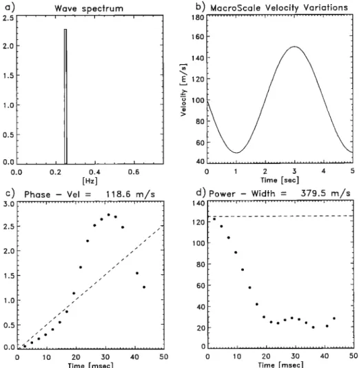
4.2.1. Autocorrelation function. Figure 1 gives an ex- ample of a simulated ACF when considering a monochro-

27,084 ANDRI• ET AL.' LOW-ALTITUDE CUSP SEEN BY HF RADARS a) 2.0 1.5 1.0 0.5 0.0 0.0 c) 2.5 2.0 1.5 1.0 0.5 Wave spectrum 0.2 0.4 0.6 [•] Phase - Vel- 118.6 m/s

...

i ...

vl

...

[

...

i ...

b) MacroScale

Velocity

Variations

180 ... ' ... ' ... • ... ' ... "• 160 60 140 0 1 2 3 4 5 Time [sec]

d) Power- Width -

379.5 m/s

ß

ß

ß

ß

ß

ß

ß

ß ß

ß

...

,1,,i

...

,,,i,,,,1,,,,•

...

i ...

Figure

1. (a) Spectrum

of the monochromatic

wave

used,

(b) Velocity

variation

during

the

radar

integra-

tion time, (c) Phase of the simulated autocorrelation function (ACF), (d) Power of the simulated ACE

matic wave defined by an amplitude of 50 m s -t, a fre-

quency of 0.250 Hz, and 90øphase offset (½k), in a back-

ground plasma velocity of 100 m s- 1 along the radar beam

direction. The wave frequency spectrum and the induced velocity variation during the integration time are shown in Figures 1 a and lb, respectively, and the temporal evolution of the phase and power of the ACFs are plotted in Figure l c and ld, respectively. If the velocity spectrum comprised a single component, it would produce a linear progression of phase with time (lag), as shown by the dotted line. The

phase progression is not linear. This modulation, also seen

in the power, suggests that the spectrum associated with this ACF contains several velocity components. A Fourier analy- sis (not shown) shows a spectrum with several velocity com- ponents which can be different from those experienced by the irregularities, and these components are therefore arte- facts of the data processing. This spectrum is very similar to those published by Baker et al. [1995]. The velocity de-

duced from the phase (118 m s -1) is close to the defined

background velocity (100 m s -1), but despite the fact that

there is no turbulent effect in this simulation, such a tempo- ral variation of the electric field introduces a spectral width

of 376 m s-•.

4.2.2. Velocity aliasing. Figure 2a shows the velocity

found by FITACF as a function of varying the wave phase (½k) in (1). The upper curve corresponds to a velocity mod-

ulation with an amplitude of 50 m s-t, a frequency of 0.5 Hz

in a background velocity of 200 m s -t, whereas the lower

curve results from a wave which has an amplitude and a fre-

quency

of 50 m s -1 and 0.15 Hz, respectively,

in a back-

ground plasma velocity of 75 m s-•. The bars show the er-

rors on the velocity determined by the FITACF method. The velocity is seen to vary with the wave phase, but it is still in- side the velocities experienced by the scatterers (e.g., 200 4-

50 m s-t), whatever

the background

velocity

used.

The ve-

locity errors are less than 30 m s- 1 and do not seem to vary

with the frequency of the wave, but they can be much smaller for some phase shifts. The main feature of these curves is the bimodal characteristic of the derived velocity values, seen particularly clearly in the case for a background flow of 75 m

s -t. The derived velocity values switch rapidly, for a small

change in phase, between an upper and lower velocity value. We next explore the consequences of this behavior.

With such a wave model, one can produce time series of ionospheric velocity variations from which the ACFs can be computed (with the radar running in a high-resolution mode:

ANDR15. ET AL.' LOW-ALTITUDE CUSP SEEN BY HF RADARS 27,085 300 ... • ... • ... • .... 250

.__>.

15o

a

•ooo

•_

,

,

'

400

Figure

2. (a) Velocity

determined

by the standard

method

called

FITACF

as a function

of the

wave

phase

for a wave

frequency

and

amplitude

of 0.15 Hz and

50 m s-•, respectively,

for the lower

curve

and

of 0.5

and

50 m s

-• for the

upper

curve.

The

background

velocities

are

200

and

75 m s

-• for the

upper

curve

and

the lower

curve,

respectively.

(b) Fluctuation

frequency

of the determined

velocity

as a function

of

the wave frequency. (c) As in Figure 2a but for the spectral width.

5-s integration time, with a temporal resolution of 10 s) and finally arrive at the velocities determined by the radar for each integration period. Because the phase of the wave will vary between two successive integration times, the computed

velocity will be different, and hence one might expect a mod- ulation in the velocities determined by the radar.

Figure 2b presents the modulation frequency discussed above as a function of the wave frequency used in the simu-

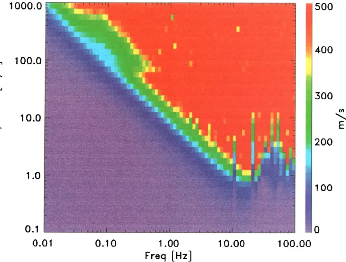
27,086 ANDRI2 ET AL.: LOW-ALTITUDE CUSP SEEN BY HF RADARS 1000.0 lOO.O II ill !1 0.01 0.10 1.00 10.00 100.00

Freq [Hz]

Plate 1. Color-coded spectral width as a function of the wave amplitude and wave frequency. 5OO 400 300 2OO lOO o

lation. Figure 2b shows a typical aliasing effect in the veloc- ity determination. In the radar's high-resolution mode the temporal resolution gives a Nyquist frequency of 50 mHz.

In the common radar running mode the temporal resolution

of the velocity is 2 min, which implies a Nyquist frequency of 4 mHz. All the waves which have a frequency lower than

the Nyquist frequency are correctly resolved by the radar,

but the highest frequency waves are undersampled. Thus a typical Pc 1 wave could be seen as a Pc5 wave in the radar

data. We stress that this behavior can only be demonstrated

for a monochromatic Pc 1 wave.

Figure 2c shows the spectral width as a function of the wave phase. When the wave frequency is 0.15 Hz (lower

curve), the spectral width is nearly constant around 200 m

s -1, with a small error (_< 50 m s -x). When the frequency

increases (upper curve is for 0.5 Hz), the spectral width val- ues increase and become much more variable with phase,

covering the range 200-900 m s -x, and their associated er-

rors are higher, reaching 100 m s -•. In summary, Figure

2 shows that the radar determines a velocity value which is

representative of the convection conditions (i.e., within the background velocity value and the wave amplitude), but the spectral width determined is strongly dependent on the fre-

quency of the perturbing wave.

4.2.3. High spectral width. Plate 1 shows the mean

spectral width values (color-coded) as a function of the wave frequency and wave amplitude. For each possible combina-

tion of frequency and amplitude the temporal variability of the ionospheric plasma velocity has been determined for a set period of time, and then this time series has been passed through the simulator. The resulting ACFs are then analyzed by FITACF, and spectral width values are produced. Thus, for a given wave frequency and amplitude, one has a spectral

width distribution that is representative of the different wave phase encountered and its mean value over the set period of

time.

Plate 1 shows a sharp transition between low and high

spectral width. For example, when the wave amplitude is of

the order of 20 m s -• (corresponding to an electric field of

1 mV m -•), a high

mean

spectral

width

value

(greater

than

200 m s-•) is obtained

when

considering

a wave

frequency

greater than 0.8 Hz. When the wave frequency increases still further, the mean spectral width reaches a saturation level at

around

650 m s

-1 . Correspondingly,

for a given

wave

fre-

quency a greater spectral width value is obtained with in-

creasing wave amplitude.

The main property of this result is that except for low- frequency (f < 0.5 Hz) and large amplitude (V1 >

ANDRI• ET AL.: LOW-ALTITUDE CUSP SEEN BY HF RADARS 27,087

80 m s -t) waves, the transition from low to high spectral

width is sharp and occurs for low-amplitude waves (for ex-

ample,

at 20 m s

-t = 1 mV m -x for 0.5 Hz). For lower-

frequency

waves

the high

spectral

width

regime

is obtained

more progressively and for higher wave amplitude (200 m

s -x = 10 mV m -t for 0.1 Hz).

4.3. Narrowband Wave

Waves seen on the ground near the cusp have a bandwidth

of the order of 0.2 Hz [Dyrud et al., 1997], which is narrower

near

the equatorward

edge

of the cusp

and

wider

on its pole-

ward edge. This suggests that a more realistic simulation

would be to consider the case of a narrowband electric field.

To achieve this, the spectrum is simulated by the addition

of 500 monochromatic waves which have the same ampli- tude• The distribution function of the wave frequencies is then centered around a main frequency and is characterized by a spectral width.

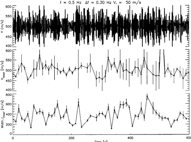
4.3.1. Time series. From this wave model, one can gen-

erate long time series (10 min) of ionospheric plasma veloc-

ities and compute the velocity and the spectral width. Figure

3 shows on the upper panel an example of a time-varying

electric field generated by this simulation. Here the mean

wave amplitude,

wave frequency,

and band

width are 2.5

mV m -• (which

corresponds

to a velocity

of 50 m s

-•),

0.5 Hz, and 0.3 Hz, respectively. The background line-of-

sight

velocity

is set

to 500 m s-•. Examining

the

ACF

phase

plots

(not shown)

produced

for each

integration

period

from

this simulation shows a strong nonlinear behavior, suggest-

ing that

the spectra

associated

with these

ACFs

contain

sev-

eral components.

The middle

and

lower

panels

of Figure

3

show

the Doppler

velocity

(middle

panel)

and

the spectral

width (lower

panel)

values

produced

by the radar's

signal

processing.

The error

bars

show

the statistical

uncertainties

associated

with these

parameters,

derived

by the standard

fit-

ting

procedure

(FITACF).

Figure

3 illustrates

well the vari-

ability

obtained

in both

the

Doppler

velocity

and

the

spectral

width,

and

the

high

spectral

width

values

(• 400

m s

-t).

These variations are typical of the radar data seen in the

cusp.

For example,

Figure

4 shows

the

line-of-sight

velocity

(upper

panel)

and

the spectral

width

(lower

panel)

recorded

by the Halley

SuperDARN

radar

during

10 min,

in two dif-

ferent range gates located inside and equatorward of the cusp

(the upper and lower curves, respectively). The upper curve

has

been

shifted

by 500 m s- t for clarity

and

shows

a highly

variable

spectral

width,

with

an

average

value

of 400

m s-t,

in good

agreement

with the simulated

results

(Figure

3).

4.3.2. Wave amplitude effect. We next show the gen-

erality

of the results

obtained

in Figure

3 by varying

both

the background

line-of-sight

velocity

and

the amplitude

of

the perturbing wave. From such time series, one can com-

pute

the

mean

Doppler

velocity

and

spectral

width

with

their

corresponding

standard

deviations,

when

considering

a par-

ticular

wave frequency

and bandwidth

(0.5 and 0.235 Hz,

respectively) for several wave amplitudes.

Figure

5 (left) shows

the mean

velocity

as a function

of

f = 0.5 Hz Af = 0.30 Hz V, 50 m/s 600 550 ,•E 500 450 4O0 600 550 500 45O 40O 80O 600 400 200 0 200 40o 6()0 Time Is]

Figure 3. From top to bottom,

time series

of the wave

induced

velocity

field, simulated

line-of-sight

27,088 ANDRI• ET AL.: LOW-ALTITUDE CUSP SEEN BY HF RADARS

HALLEY STATION, 22 December 1995, Beam 8, Ranges' 22, 26

1000 500 0

-500

: -

-

400

200

Figure 4. Velocity (upper panel) and spectral width (lower panel) recorded at Halley on December 22, 1995, inside the cusp (upper curve) and equatorward of it (lower curve). The upper curves have been

shifted by 500 m s- • for clarity.

1500 lOOO 500 Broadband wave f - 0.,50 Hz - w-- 0.235 Hz f = 0.50 Hz - w= 0.235 Hz Vo = 1000 Vo = 500 Vo = 100 1500 •E 1000 ._ 5OO i , , , I , , , , I , , , , 0 I , , , t 0 50 100 150 0 50 100 150 V, [m/s] V, [m/s]

Figure 5. (left) Mean value of the velocity and (right) spectral width. Both values are shown as a function

of the wave amplitude and for several background velocities. The error bars give the standard deviations

ANDRI2 ET AL.' LOW-ALTITUDE CUSP SEEN BY HF RADARS 27,089 3OO 200 lOO

Vel [m/s]

Width [m/s]

Figure 6. (left) Mean value of the velocity and (right) the spectral width. Both values are shown as a function of the wave amplitude and for wave frequency. The error bars give the standard deviations

associated with the mean values.

the wave amplitude (frequency, 0.5 Hz; bandwidth, 0.235 Hz), for three background line-of-sight velocities. The error bars represent the standard deviation of these averaged val- ues and so give us an estimate of the velocity fluctuations. The mean velocity does not depend on the wave amplitude. The variations also increase with the wave amplitude, but they are still in the range of the velocity experienced by the

scatterers. The conclusion reached is that the mean velocity

corresponds to the background velocity whatever the wave amplitude but that the velocity fluctuations increase with the

wave amplitude.

Figure 5 (right) shows the spectral width (determined by applying a Lorentzian fit on the ACF power) as a function of the wave amplitude and for the same background velocities as before. One has to note that the curves which correspond

to a background

velocity

of 500 and 1000

m s -1 have

been

shifted

by 500 and 1000 m s -1, respectively,

for clarity.

It

shows that regardless of the background line-of-sight veloc-

ity value,

a small

wave

amplitude

(1 mV m -1 = 20 m s -1)

can

result

in a spectral

width

value

of 200 m s -x or greater.

Again, the fluctuations of the determined spectral width in- crease with the wave amplitude. This result is very similar

to the one found with monochromatic waves.

4.3.3. Wave frequency effect. One can also investigate the variations of these parameters as a function of wave fre- quency. Here one considers a wave bandwidth equal to 0.1

times the main frequency used. The wave amplitude is 2.5

mV m -1 (50 m s-•), and the background

velocity

is 100 m

-1 S .

Figure 6 (left) shows the averaged velocity and its stan- dard deviation as a function of wave frequency. The velocity

is constant when the wave frequency is lower than 2 Hz, with

a standard deviation which agrees well with the wave ampli- tude considered. When the wave frequency increases above 2 Hz, the mean velocity starts to be highly variable, with a very large standard deviation, typically greater than 150 m

s -1. This shows

that the velocities

recorded

are no longer

representative of the real background velocity of 100 m s-1.

Howerver, these erroneous velocities can easily be detected by checking their associated error, which is greater than 100

m s-l, the threshold

usually

taken

when

analyzing

real

radar

data [Baker et al., 1995].

Figure 6 (right) shows the mean value of the spectral width as a function of the wave frequency. The spectral

width

is greater

than 150 m s -1 for frequencies

greater

than

0.2 Hz and sharply increases with frequency until a satura- tion level is reached. This limitation appears at around 650

m s -1 for frequencies

greater

than • 1.3 Hz. Thus,

even

for a low-amplitude

narrowband

wave

(2.5 mV m-l) in the

Pc 1-Pc2 frequency band, a high value of spectral width is

obtained.

27,090 ANDRI2 ET AL.' LOW-ALTITUDE CUSP SEEN BY HF RADARS plitude varies, but the erroneous velocities and the spectral

width saturation at 650 m s-1 are obtained for different fre-

quencies, 3 and 2 Hz, respectively, for a wave amplitude of

1.25 mV m -1, or 1 and 0.8 for a wave amplitude of 5 mV

--1 m .

These results are very similar to those obtained when con- sidering a monochromatic wave. This suggests that the wave bandwidth does not strongly affect these profiles but can only slightly decrease or increase the spectral width because of the differing contribution of the highest frequencies in the

wave spectrum.

One can conclude that the results shown in Plate 1 are still valid for a more realistic case. When the saturation level is

reached, one can observe a strong increase of the error in the

velocity determination.

5. Discussion

5.1. Limitations

The decay time of the ACF power, quantified by the spec- tral width, reflects the typical correlation time between ir- regularity motions under a turbulent electric field. In this

simulation the scatterers are randomly distributed over one

range gate, and they experience the same electric field. This implies that they keep their coherence all the time, and thus, when considering a steady electric field, the spectral width

is expected

to be equal

to 0 m s -• .

It is assumed that there are no structures of the scale size

of an HF radar sampling cell (typically 50 x 100 km) in the ionosphere, resulting from smaller-scale and intense precip-

itations, or static structure in the electric field. These struc-

tures would increase the width of the velocity distribution

in the radar range gate, and thus they should also increase the spectral width recorded by the radar. Because the same electric field is applied to all irregularities, it is assumed that the wavelength perpendicular to the magnetic field is much greater than the gate length. A smaller wavelength will increase the spatial inhomogeneities and thus the spec-

tral width.

In this simulation the irregularities are uniformly dis-

tributed over the whole radar range gate, and their amplitude

is constant. Thus the amplitude of the signal backscattered by each irregularity is assumed to be the same. This may not be the case in the F region ionosphere. The irregularities are likely to vary in amplitude within a range gate, and thus the backscattered power is more likely to come from several areas located inside the range gate. By assuming that it is

coming mainly from one single area, one could extend this

simulation to smaller wavelengths. These limitations imply

that the results obtained in this study should be considered

as the minimum values of the spectral width recorded by HF

radar in the cusp region.

5.2. Wave Source

We have shown that any kind of electric field variation at low altitude (ionospheric F region), in the frequency band

0.1-100

Hz and with a sufficient

amplitude

(a few mV m -1)

leads to a high spectral width in the SuperDARN radar data. Limitations cited in section 5.1 suggest that the wave should have a wavelength perpendicular to the magnetic field greater than the radar gate length (45 km). Wave obser- vations in the cusp can generally be described as a super- position of narrowband waves, such as ion cyclotron waves

around 1 Hz and a broadband wave.

5.2.1. Broadband electromagnetic noise. Low-

frequency electromagnetic noise is observed in the auroral

zone [Gurnett et al., 1984; Gumerr, 1991]. Electric and

magnetic spectra are characterized by a power law, with a magnetic spectrum steeper than the electric one, especially at frequencies greater than 10 Hz. Both electric and magnetic fields are perpendicular to the ambient magnetic field, and the Poynting flux is directed earthward. Several attempts have been made to distinguish between fields from static structures and waves [e.g., Gurnett et al., 1984;

Weimer et aL, 1985; Berthelier et al., 1991; Heppner et al.,

1993].

In the first interpretation (fields from static structures),

electric fields are generated by the closure of fi. eld-aligned

currents in the E region whereas magnetic variations are pro- duced directly by these currents. In this model, the magnetic to electric field ratio is expected to be related to the height-

integrated Pedersen conductivity. In this case the observed

wave does not correspond to a temporal variation of the elec-

tric field, and thus this wave cannot be used as the energy

source of the high radar spectral width.

The noise can also be interpreted as propagating Alfv6n waves generated at the magnetopause or in the distant mag-

netotail. In this case the E/B ratio should be of the order

of the local Alfvdn wave velocity [Lysak and Dum, 1983]. In a detailed study, Wahlund et al. [1998] have shown that this noise is probably due to a superposition of several wave modes. At the lowest frequencies (below a few tens of hertz) the wave is mainly Alfvdnic, as it has been also shown by Chmyrev et al. [1985], Knudsen et al. [1990], Matsuoka et al. [ 1993], and later by Keady and Heelis [ 1999].

Similar noise has been recorded within the region of au- roral inverted-V electron precipitation and has also been as-

sociated with intense events of transverse ion acceleration

[e.g., Andrd et al., 1990; Norqvist et al., 1996]. Later, some studies have shown that resonant heating by broadband low-

frequency waves is the dominant ion energization mecha-

nism [Andrd et al., 1998; Knudsen et al., 1998; Norqvist

et al., 1998].

5.2.2. Narrowband wave. Narrowband waves at fre-

quencies lower than 10 Hz are usually referred to as Pc l waves and have been observed on the ground [e.g., Menk

et al., 1992; Dyrud et al., 1997, and references therein], at

low altitudes [Iyemori and Hayashi, 1989; Erlandson et al.,

1993; Iyemori et al., 1994], high altitudes [Erlandson et al.,

1990], and in the equatorial plane of the magnetosphere [An- derson et al., 1992]. This Pcl wave activity is a persistent feature at ionospheric altitudes over the whole cusp, but its ground signature does not appear so often and seems to be localized on the cusp boundaries only, with a narrowband

ANDRI• ET AL.' LOW-ALTITUDE CUSP SEEN BY HF RADARS 27,091

wave near the low-latitude boundary layer and a wideband emission near the poleward edge of the cusp [e.g., Dyrud

et al., 1997].

Most of these waves are attributed to electromagnetic ion

cyclotron waves generated at the dayside magnetopause in the equatorial plane, which propagate in the slow Alfvfin wave mode along the magnetic field lines to the ionosphere [e.g., Basinska et al., 1994]. However, they could be gen-

erated during reconnection processes at the magnetopause

and propagate along the newly reconnected magnetic field lines. They could also be generated by the reflected cusp ions propagating upward near the poleward edge of the cusp [Dyrud et al., 1997]. These propagating waves could then be reflected by the conducting ionosphere or alternatively by the sharp gradient in the Alfv•n velocity found around 1 RE. This cavity, termed the ionospheric Alfv•n resonator, traps Alfv•n waves in the frequency range 0.1-1.0 Hz. This im- plies that waves found at ionospheric altitudes in this fre- quency band should be composed of a mixture of upgo- ing and downgoing Alfv•n waves [Polyakov and Rapoport,

1981].

Recently, Lysak [ 1999] modeled Alfv•n wave propagation through the ionosphere and showed that waves generated at high altitude can reach the ground when their frequency matches a normal mode of the ionospheric resonator. He also found that the typical perpendicular wavelength is in the range 500-1000 km in the frequency band 0.5-1 Hz.

5.2.3. High spectral width. These studies show that the low-frequency part of the wave spectrum recorded in the cusp on board low-altitude satellites comprises a super- position of bouncing Alfvdn waves and the effect of static field-aligned cmTents. Because this last component does not imply a temporal variation of the electric field, the Alfvdn wave contribution is likely to be the main energy source which gives rise to the high spectral width in the radar data. This is strengthened by their persistent appearance and their large perpendicular wavelength. Because these waves are strongly related to the cusp location, one can conclude that as it has been experimentally shown by Baker et al. [1995], high spectral width in the radar data is a good proxy of the

crisp location.

6. Conclusion

Identification of the ionospheric signature of the cusp is important since it is a proxy of the open/closed field line boundary on the dayside. By comparison with low-altitude

satellite data and optical imagers, Baker et al. [ 1990, 1995],

Rodger et al. [1995] and Yeoman et al. [1997] have exper- imentally shown that this region is characterized in the HF radar data by a high spectral width. This signature has been extensively used to study the dynamics of the cusp or pro- cesses connected with magnetic reconnection [e.g., Pinnock et al., 1995, 1999; Baker et al., 1997; Milan et al., 1999;

Greenwald et al., 1999]. However, none of these studies

have explained why the spectral width is high in this region.

In this paper we have evaluated the impact of a time- varying electric field in the radar data and especially on the

spectral width. We have shown that a narrowband wave in

the Pc 1 frequency band, even with a low amplitude, leads to the ACF characteristics observed in the cusp: a great vari- ability in the determined parameters, a spectrum which con- tains several components, and a high spectral width value. One has to note that this wave activity does not strongly affect the determination of the background electric field and that supplementary components in the recorded Doppler spectrum are caused by the radar technique and may be arte-

facts.

Because several studies have already shown that such a wave activity is continuously seen in the cusp by low- altitude satellites [Curtis et al., 1982; Maynard, 1985; May-

nard et al., 1991; Matsuoka et al., 1991, 1993; Erlandson

and Anderson, 1996] and that its main component at low frequencies could come from downward propagating Alfvdn

waves, one can conclude that these waves are the main

source of the high spectral width observed in the radar data. This wave activity is also observed on magnetic field lines in the auroral oval [Gurnett, 1991]. Thus one can prob- ably use the same mechanism to explain the high spectral widths found over the whole auroral zone, and especially in the nightside where a smooth increase of the spectral width has been associated with the boundary between the central plasma sheet/plasma sheet boundary layer [Dudeney et al., 1998]. Following Gary et al. [ 1998], this wave activity could also be the signature of the boundaries of large-scale, field- aligned current systems. We conclude that HF radars are able to reveal sites of wave activity (electromagnetic or elec- trostatic) in the low-altitude ionosphere and that this poten- tial can be used to map some magnetospheric boundaries.

Acknowledgments. The authors acknowledge helpful discus-

sions with J.-P. Villain and C. Hanuise. This work has been funded

by the European Community grant ERB4001GT973635.

Michel Blanc thanks Patrick T. Newell and Nelson C. Maynard

for their assistance in evaluating this paper.

References

Anderson, B.J., R.E. Erlandson, and L.J. Zanetti, A statistical study of Pc 1-2 magnetic pulsations in the equatorial magnetosphere, 1,

Equatorial occurrence distributions, J. Geophys. Res., 97, 3075-

3088, 1992.

Andr6, M., G.B. Crew, W.K. Peterson, A.M. Persoon, C.J. Pollock,

and M.J. Engebretson, Ion heating by broadband low-frequency waves in the cusp/cleft, J. Geophys. Res., 95, 20,809-20,823,

1990.

Andr6, M., P. Norqvist, L. Andersson, A.I. Eriksson, L. Blomberg, R.E. Efiandson, and J. Waldemark, Ion energization mechanisms at 1700 km in the auroral region, J. Geophys. Res., 103, 4199-

4222, 1998.

Andr6, R., J.-P. Villain, C. Senior, L. Barthes, C. Hanuise, J.- C. Cerisier, and A. Thorolfsson, Toward resolving small-scale

structures in ionospheric convection from SuperDARN, Radio

Sci.,34, 1165-1176, 1999.

Baker, K.B., R.A. Greenwald, J.M. Ruohoniemi, J.R. Dudeney, M. Pinnock, P.T Newell, M.E. Greenspan, and C.-I. Meng, Si- multaneous HF-radar and DMSP observations of the cusp, Geo- phys. Res. Lett., I7, 1869-1872, 1990.

Baker, K.B., J.R. Dudeney, R.A. Greenwald, M. Pinnock, P.T Newell, A.S. Rodger, N. Mattin, and C.-I. Meng, HF radar sig-

27,092 ANDRI2 ET AL.: LOW-ALTITUDE CUSP SEEN BY HF RADARS

natures of the cusp and low-latitude boundary layer, J. Geophys.

Res., 100, 7671-7695, 1995.

Baker, K.B., A.S. Rodger, and G. Lu, HF-radar observations of the dayside magnetic merging rate: A Geospace Environment Modeling boundary layer campaign study, J. Geophys. Res., 102,

9603-9617, 1997.

Barthes, L., R. Andr6, J.-C. Cerisier,,and J.-P. Villain, Separation of multiple echoes using a high resolution spectral analysis in SuperDARN HF radars, Radio Sci., 33, 1005-1017, 1998. Basinska, E.M., W.J. Burke, N.C. Maynard, W.J. Hughes, D.J.

Jnudsen, and J.A. Slavin, Electric and magnetic field fluctua- tions at high-latitudes in the dayside ionosphere during south- ward IMF, in Solar Wind Sources of Magnetospheric Ultra-Low- Frequency Waves, Geophys. Monogr. Set., vol. 81, edited by M.J. Engebretson, K. Takahashi, and M. Scholer, pp. 387-397, AGU, Washington, D.C., 1994.

Berthelier, A., J.-C. Cerisier, J.-J. Berthelier, and L. Rezeau, Low-

frequency magnetic turbulence in the high-latitude topside iono- sphere: Low-frequency waves or field-aligned currents, J. At- mos. Terr. Phys., 53, 333-341, 1991.

Bolshakova, O.B., V.A. Troitskaya, and K.G. Ivanov, High-latitude Pc 1-2 geomagnetic pulsations and their connection with location of the dayside polar cusp, Planet. Space Sci., 28, 1-7, 1980. Chmyrev, V.M., V.N. Oraevsky, S.V. Bilichenko, N.V. Isaev, G.A.

Stanev, D.K. Teodosiev, and S.I. Shkolnikova, The fine structure

of intensive small-scale electric and magnetic fields in the high- latitude ionosphere as observed by Intercosmos-Bulgaria 1300 satellite, Planet. Space Sci., 33, 1383-1388, 1985.

Curtis, S.A., W.R. Hoegy, L.H. Brace, N.C. Maynard, M. Sugiura, and J.D. Winningham, DE-2 cusp observations: Role of plasma instabilities in topside ionospheric heating and density fluctua- tions, Geophys. Res. Lett., 9, 997-1000, 1982.

Dudeney, J.R., A.S. Rodger, M.P. Freeman, J. Pickett, J. Scudder, G. Sofko, and M. Lester, The nightside ionospheric response to IMF By changes, Geophys. Res. Lett., 25, 2601-2604, 1998. Dyrud, L.P., M.J. Engebretson, J.L. Posh, W.J. Hughes, H. Fuku-

nishi, R.L. Arnoldy, P.T. Newell, and R.B. Horne, Ground ob- servations and possible source regions of two types of Pc 1-2 micropulsation at very high-latitudes, J. Geophys. Res., 102,

27,011-27,027, 1997.

Dyrud, L.P., M.J. Engebretson, J.L. Posh, W.J. Hughes, H. Fuku- nishi, R.L. Arnoldy, and P.T Newell, Conjugate ground obser- vations and possible source regions of two types of Pc 1-2 pulsa- tions at very high-latitudes, in Polar Cap Boundary Phenomena,

edited by J. Moen, A. Egeland, and M. Lockwood, pp. 311-326,

Kluwer Acad., Norwell, Mass., 1998.

Erlandson, R.E., and B.J. Anderson, Pc 1 waves in the ionosphere:

A statistical study, J. Geophys. Res., 101, 7843-7857, 1996. Erlandson, R.E., L.J. Zanetti, T.A. Potemra, L.P. Block, and

G. Holmgren, Viking magnetic and electric field observations of Pc 1 waves at high-latitudes, J. Geophys. Res., 95, 5941-5955,

1990.

Erlandson, R.E., T.L. Aggson, W.R. Hoegy, and J.A. Slavin, Si- multaneous observations of subauroral electron temperature en-

hancements and electromagnetic ion cyclotron waves, Geophys.

Res. Lett., 20, 1723-1726, 1993.

Gary, J.B., L.J. Zanetti, B.J. Anderson, TA. Potemra, J.H. Clem- mons, J.D. Winningham, and J.R. Sharber, Identification of au- roral oval boundaries from in situ magnetic field measurements, J. Geophys. Res., 103, 4187-4197, 1998.

Greenwald, R.A., K.B. Baker, R.A. Hutchins, and C. Hanuise, An HF phased array radar for studying small-scale structure in the high-latitude ionosphere, Radio Sci., 20, 63-79, 1985.

Greenwald, R.A., W.A. Bristow, G.J. Sofko, C. Senior, J.-C. Cerisier, and A. Szabo, Super Dual Auroral Radar Network radar imaging of dayside high-latitude convection under northward in-

terplanetary magnetic field: Toward resolving the distorted two- cell versus multicell controversy, J. Geophys. Res., 100, 19,661-

19,674, 1995.

Greenwald, R.A., J.-M. Ruohoniemi, K.B. Baker, W.A. Bristow, G.J. Sofko, J.-P. Villain, M. Lester, and J. Slavin, Convective

response to a transient increase in dayside reconnection, J. Geo- phys. Res., 104, 10,007-10,015, 1999.

Gurnett, D.A., Auroral plasma waves, in Auroral Physics, edited by C.-I. Meng, M.J. Rycroft, and L.A. Franck, chap. IV-6, pp. 241-254, Cambridge Univ. Press, New York, 1991.

Gurnett, D.A., R.L. Huff, J.D. Menietti, J.L. Burch, J.D. Winning- ham, and S.D. Shawhan, Correlated low-frequency electric and magnetic noise along the auroral field lines, J. Geophys. Res., 89,

8971-8985, 1984.

Heppner, J.P., M.C. Liebrecht, N.C. Maynard, and R.F. Pfaff, High- latitude distribution of plasma waves and spatial irregularities from DE 2 alternating current electric field observations, J. Geo- phys. Res., 98, 1629-1652, 1993.

Iyemori, T., and K. Hayashi, Pc l micropulsations observed by MAGSAT in the ionospheric F region, J. Geophys. Res., 94, 93-

100, 1989.

Iyemori, T., M. Sugiura, A. Oka, Y. Morita, M. Ishii, J.A. Slavin, L.H. Brace, R.A. Hoffman, and J.D. Winningham, Localized in- jection of large amplitude Pc l waves and electron temperature

enhancement near plasmapause observed by DE 2 in the upper ionosphere, J. Geophys. Res., 99, 6187-6199, 1994.

Keady, J.P., and R.A. Heelis, Regional, scale size, and interplan- etary magnetic field variability of magnetic field and ion drift structures in the high-latitude ionosphere, J. Geophys. Res., 104,

199-212, 1999.

Knudsen, D.J., M.C. Kelley, G.D. Earle, J.F. Vickrey, and M. Boehm, Distinguishing Alfv•n waves from quasi-static field structures associated with the discrete aurora: Sounding rocket and HILAT satellite measurements, Geophys. Res. Lett., 17,

921-924, 1990.

Knudsen, D.J., J.H. Clemmons, and J.-E. Wahlund, Correlation be-

tween ion energization, suprathermal electron burst, and broad- band ELF plasma waves, J. Geophys. Res., 103, 4171-4186,

1998.

Lysak, R.L., Propagation of Alfv•n waves throughout the iono- sphere: Dependence on ionospheric parameters, J. Geophys.

Res., 104, 10,017-10,030, 1999.

Lysak, R.L., and C.T Dum, Dynamics of magnetosphere- ionosphere coupling including turbulent transport, J. Geophys.

Res., 88, 365-380, 1983.

Matsuoka, A., T. Mukai, H. Hayakawa, Y.-I. Kohno, K. Tsuruda, A. Nishida, T Okada, N. Kaya, and-H. Fukinishi, EXOS-D ob- servations of electric field fluctuations and charged particle pre-

cipitation in the polar cusp, Geophys. Res. Lett., 18, 305-308,

1991.

Matsuoka, A., K. Tsuruda, H. Hayakawa, T. Mukai, A. Nishida, T. Okada, N. Kaya, and H. Fukunishi, Electric field fluctuations

and charged particle precipitation in the cusp, J. Geophys. Res.,

98, 11,225-11,234, 1993.

Maynard, N.C., Structure in the DC and AC electric fields associ- ated with the dayside cusp region, in The Polar Cusp, edited by J.A. Holtet and A. Egeland, pp. 305-322, D. Reidel, Norwell,

Mass., 1985.

Maynard, N.C., TL. Aggson, E.M. Basinka, W.J. Burke, P. Craven, W.K. Peterson, M. Sugiura, and D.R. Weimer, Magnetospheric boundary dynamics: DE-1 and DE-2 observations near the mag- netopause and cusp, J. Geophys. Res., 96, 3505-3522, 1991.

Menk, F.W., B.J. Fraser, H.J. Hansen, P.T. Newell, C.-I. Meng, and R.J. Morris, Identification of the magnetospheric cusp and cleft using Pc 1-2 ULF pulsations, J. Atmos. Terr. Phys., 54, 1021-

1042, 1992.

Milan, S.E., M. Lester, S.W.H. Cowley, J. Moen, P.E. Sandholt, and C.J. Owen, Meridian-scanning photometer, coherent HF radar, and magnetometer observations of the cusp: a case study, Ann. Geophys., 17, 159-172, 1999.