HAL Id: hal-02927414
https://hal.archives-ouvertes.fr/hal-02927414
Submitted on 19 Oct 2020
HAL is a multi-disciplinary open access
archive for the deposit and dissemination of
sci-entific research documents, whether they are
pub-lished or not. The documents may come from
teaching and research institutions in France or
abroad, or from public or private research centers.
L’archive ouverte pluridisciplinaire HAL, est
destinée au dépôt et à la diffusion de documents
scientifiques de niveau recherche, publiés ou non,
émanant des établissements d’enseignement et de
recherche français ou étrangers, des laboratoires
publics ou privés.
Abrupt decline in tropospheric nitrogen dioxide over
China after the outbreak of COVID-19
Fei Liu, Aaron Page, Sarah A. Strode, Yasuko Yoshida, Sungyeon Choi, Bo
Zheng, Lok Nath Lamsal, Can Li, Nickolay A. Krotkov, Henk J. Eskes, et al.
To cite this version:
Fei Liu, Aaron Page, Sarah A. Strode, Yasuko Yoshida, Sungyeon Choi, et al.. Abrupt decline in
tropospheric nitrogen dioxide over China after the outbreak of COVID-19. Science Advances ,
Amer-ican Association for the Advancement of Science (AAAS), 2020, 6 (28), pp.eabc2992.
�10.1126/sci-adv.abc2992�. �hal-02927414�
Cite as: F. Liu et al., Sci. Adv 10.1126/sciadv.abc2992 (2020).
RESEARCH ARTICLES
First release: 12 June 2020 www.advances.sciencemag.org (Page numbers not final at time of first release) 1
Introduction
In December 2019, a respiratory disease, coronavirus disease 2019 (COVID-19), emerged in Wuhan City, Hubei Province, China (1). COVID-19 has since spread worldwide causing tens of thousands of deaths (2). To combat the spread of COVID-19, the Chinese government sealed off several cities reporting large numbers of infected people, including Wuhan, starting January 23, 2020; this included halting public transportation and closing local businesses. These prevention efforts quickly expanded nationwide. The policy announcements and restrictions, applied at an unprecedented scale, have implications for the Chinese environment and the economy that we quantitatively evaluate in this paper. In particular,
we use satellite nitrogen dioxide (NO2) measurements to
monitor changes in fossil fuel usage, related to economic activity, over China following the outbreak of COVID-2019.
Nitrogen oxides (NO + NO2 = NOx), emitted during high
temperature combustion, are relatively short-lived in the atmosphere (lifetimes of the order of hours near the surface),
and therefore remain relatively close to their sources (3). NO2
tropospheric vertical column density (TVCD) retrieved from backscattered solar radiation, such as from the Ozone Monitoring Instrument (OMI) (4), has been widely used to monitor both long term and short-term changes in fuel consumption (5, 6). OMI’s successor, the Tropospheric Monitoring Instrument (TROPOMI) (7) offers a higher spatial
resolution measurement of NO2 TVCD.
Results and Discussion
We observe substantial reductions of NO2 TVCD after the
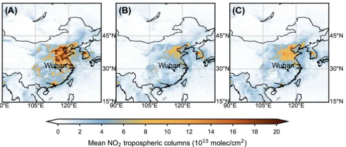
2020 Lunar New Year (LNY) on January 25, 2020. Fig. 1
shows 20-day averages of OMI NO2 TVCD before, during and
after the 2020 LNY (hereafter referred to as the “pre”, “peri”
and “post” periods). An average reduction of 48% in NO2
TVCD over China is observed from pre to peri periods.
Con-sistency in the trends of retrieved NO2 TVCD is found
be-tween OMI and its successor TROPOMI (Figure S1). A
reduction in NO2 TVCD is typically observed during LNY
be-cause most Chinese factories shut down for the holiday and the traffic volumes decrease, resulting in a decrease in fuel
consumption and thus NOx emissions. OMI NO2 TVCD shows
a pre to peri decline of 27% ± 5% (mean ± standard deviation) from data covering the 2015 to 2019 period (Fig. S2). Simi-larly, TROPOMI shows a reduction of 33% in 2019 (Fig. S3). This suggests that the observed reduction in 2020 far exceeds (21% ± 5%) the typical holiday-related pre to peri period re-duction.
Consistent with the 2015–2019 data, the 2020 NO2 TVCD
7-day moving averages show a significant reduction during approximately the two weeks leading up to LNY and reach a minimum around LNY, consistent with the gradual shut-down of factories before the holiday (Fig. 2). In prior years, a
Abrupt decline in tropospheric nitrogen dioxide over China
after the outbreak of COVID-19
Fei Liu1,2*, Aaron Page3, Sarah A. Strode1,2, Yasuko Yoshida2,4, Sungyeon Choi2,4, Bo Zheng5, Lok N. Lamsal1,2, Can Li2,6, Nickolay A. Krotkov2, Henk Eskes7, Ronald van der A7,8, Pepijn Veefkind7,9, Pieternel F. Levelt7,9, Oliver P. Hauser10†, Joanna Joiner2†
1Universities Space Research Association (USRA), Columbia, MD 21046, USA. 2NASA Goddard Space Flight Center Laboratory for Atmospheric Chemistry and Dynamics
Laboratory, Greenbelt, MD 20771, USA. 3Department of Management, University of Exeter, Exeter EX4 4PU, UK. 4Science Systems and Applications, Inc., Lanham, MD
20706, USA. 5Laboratoire des Sciences du Climat et de l’Environnement, CEA-CNRS-UVSQ, Gif-sur-Yvette, UMR 8212, France. 6Earth System Science Interdisciplinary
Center, University of Maryland, College Park, MD 20740, USA. 7Royal Netherlands Meteorological Institute (KNMI), De Bilt 3731 GA, The Netherlands. 8Nanjing University of
Information Science & Technology (NUIST), No.219, Ningliu Road, Nanjing, Jiangsu, P.R.China. 9Delft University of Technology, Delft 2628 CD, The Netherlands. 10Department of Economics, University of Exeter, Exeter EX4 4PU, UK.
*Corresponding author. Email: [email protected] †Contributed equally
China’s policy interventions to reduce the spread of the coronavirus disease 2019 have environmental and economic impacts. Tropospheric nitrogen dioxide indicates economic activities, as nitrogen dioxide is primarily emitted from fossil fuel consumption. Satellite measurements show a 48% drop in tropospheric nitrogen dioxide vertical column densities from the 20 days averaged before the 2020 Lunar New Year to the 20 days averaged after. This is 21% ± 5% larger than that from 2015–2019. We relate this reduction to two of the government’s actions: the announcement of the first report in each province and the date of a province’s lockdown. Both actions are associated with nearly the same magnitude of reductions. Our analysis offers insights into the unintended environmental and economic consequences through reduced economic activities.
Science Advances Publish Ahead of Print, published on June 12, 2020 as doi:10.1126/sciadv.abc2992
Copyright 2020 by American Association for the Advancement of Science.
on October 19, 2020
http://advances.sciencemag.org/
rebound of NO2 TVCD usually begins around 7 days after
LNY, marking the end of the holiday season. OMI and
TROPOMI (Fig. S4) NO2 TVCDs show similar temporal
pat-terns prior to 2020 with a clear reduction before LNY and an increase shortly thereafter. However, while the 2020 data show similar initial declines in the week leading up to LNY,
we do not observe the typical uptick in NO2 TVCDs starting
the week after the LNY as in previous years (Fig. 2). OMI (and
TROPOMI) NO2 TVCDs show a longer period of low values
near the minimum. Note that the 2020 data are generally lower than previous years, probably reflecting in part the ef-fects of China’s clean air policies that require installation of denitrification devices for all coal-fired power plants and ce-ment plants (8).
To rule out the possibility that the large NO2 TVCD
de-creases observed in 2020 may be driven by changes in the
meteorological conditions affecting local NOx chemistry and
NOx transport, we use Goddard Earth Observing System
cou-pled to the NASA Global Modeling Initiative (GEOS-GMI) (9) model simulations with constant emissions. We find the
sim-ulated effects of meteorology on NO2 TVCD small as
com-pared with the prolonged NO2 reduction we observe from the
pre to peri period (Fig. S5). The simulation with constant emissions shows many areas with increases from the pre to peri periods (Fig. S6). This suggests that in many areas the
actual decrease in NOx emissions may be larger than what is
inferred from the observed NO2 TVCDs.
Breaking these results down by sectors provides insights into the sources of reduction. All sectors experienced
dra-matic NO2 reductions. We compute 7-day running averages
for all OMI observations within 0.25° gridboxes that contain large power plants or other industrial plants with reported
NOx emissions > 5 Gg/yr (Fig. S7). OMI NO2 TVCD averages
for gridboxes containing power plants and those for other in-dustrial plants show similar temporal variations as the na-tional average (Fig. S8). This suggests that measures to reduce COVID-19 spread affected power generation as well as industrial production including steel, iron, and oil. Direct
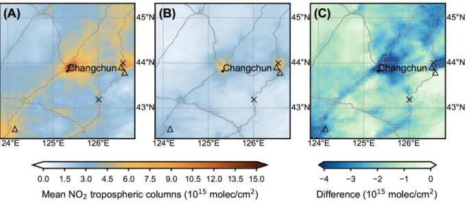
NO2 reductions from transportation are indicated by the
vis-ually reduced TROPOMI NO2 TVCDs along the China
Na-tional Highways (Fig. 3).
We next explore how COVID-19 policy interventions (most of which happened to coincide with the 2020 LNY) are
asso-ciated with reductions in NO2 TVCD. First, we consider the
announcements the government made to the public (Table S1). Once the government publicly reports that a COVID-19 case has been confirmed in a province, the public in that province might choose to reduce their exposure to others (e.g., stay at home, work from home and/or travel less). In
that case, we would expect a reduction in NO2 TVCD
follow-ing the announcement of the first case in each province. This
is indeed what we find, after taking previous years’ NO2 TVCD
and variation across provinces into account (see Eq. 1):
fol-lowing the report of the first case in each province, OMI NO2
TVCD declined by about 27% (coeff = -1.383, p = 0.002, Table 1 Col. 1).
The second policy intervention is more invasive: the gov-ernment took decisive action to further reduce the spread of the virus by limiting the mobility of citizens and locking down entire provinces; on average, lockdowns occurred 3.7 days after the report of the first case. We would expect that a lockdown would be followed by a reduction in travel as well as business activity, which in turn should lead to reductions
of NO2 TVCD. Our model (Eq. 2) shows that OMI NO2 TVCD
reduces by 24% following the lockdowns (coeff = -1.134, p < 0.001, Table 1 Col. 2).
Finally, we consider the two policies jointly (Eq. 3). We find that both the announcement of the first case reported as
well as the lockdown are associated with a reduction in NO2
TVCDs in each province (Table 1 Col. 3). These results suggest that the effect of the announcement is about as large (16%; coeff = -0.851, p = 0.043) as the effect of the lockdown (15%; coeff = -0.752, p < 0.001). All results are qualitatively similar using TROPOMI (Table S2).
NO2 reductions are closely related to improvements in air
quality (10). Under normal circumstances, many Chinese cit-ies have poor air quality that reduces life quality and
expec-tancy (11). During the COVID-19 crisis, NO2 pollution was
additionally reduced by ~20% for a period of between 30 and 50 days. While temporary, these substantial reductions in air pollution may have positive health impact for lives in other-wise heavily polluted areas (12). This unusual period offers a rare counterfactual of a potential society which uses substan-tially less fossil fuels and has lower mobility (13).
While this research provides an early insight into the NO2
changes in China in early 2020, our findings are not without
limitations. Because the relationship between NO2 TVCD and
NOx emissions is not strictly linear, the analysis of NO2 TVCD
provides a qualitative description of changes in NOx
emis-sions. Accurately quantifying the changes in NOx emissions
(14) is beyond the scope of this initial assessment.
Our results suggest that the announcement of the first
case was followed by a reduction in NO2 emissions, with a
further reduction following the actual lockdown. However, it is important to note that these results do not suggest that the mobility restrictions did not have a critical impact. Indeed, recently published work suggests that the travel restrictions in China reduced the spread of the disease by up to 80% by mid-February, in particular internationally (15). In line with our results is the finding that human mobility was reduced early on during the outbreak (16) and may in part have started as early as the first case announcements, with addi-tional reductions through lockdowns.
on October 19, 2020
http://advances.sciencemag.org/
First release: 12 June 2020 www.advances.sciencemag.org (Page numbers not final at time of first release) 3 Materials and Methods
Satellite NO2 observations
We use retrieved NO2 TVCD from both OMI and TROPOMI.
OMI is a Dutch-Finnish UV-VIS spectrometer (4) on board the US National Aeronautics and Space Administration (NASA) Aura satellite that was launched in 2004. TROPOMI is a UV-VIS-NIR-SWIR instrument (7) on board the European Copernicus Sentinel-5 Precursor satellite that was launched in 2017. Both instruments similarly measure Earth radiance and solar irradiance spectra with spectral resolutions of ap-proximately 0.5 nm. The ratio of radiance to irradiance at
wavelengths between 400 and 496 nm is used to retrieve NO2
TVCD. The ground footprint sizes are 13×24 km2 and 3.5×5.5
km2 (3.5×7 km2 before August, 2019) at nadir for OMI and
TROPOMI, respectively. Both instruments provide nearly daily to bi-daily global coverage with a local equator crossing times close to 13:30 hours. We use the version 4.0 NASA OMI
standard NO2 products (17). We use the version 1.0.0
TROPOMI Level 2 offline NO2 data products for 2019 and the
version 1.1.0 data for 2020 (18). OMI and TROPOMI measure-ments are aggregated to resolutions of 0.25°×0.25° and 0.05°×0.05°, respectively. A given gridbox value is computed by averaging the pixel-level satellite observations weighted by the amount of the pixel footprint that overlaps the gridbox. We remove OMI observations with effective cloud fractions >30% to reduce retrieval errors and those affected by the so-called “row anomaly” (19). For TROPOMI, we use only obser-vations with quality assurance values > 0.75.
For the maps shown, we calculate 20-day means of NO2
TVCD around the Lunar New Year using OMI during 2015– 2020 and TROPOMI for 2019 and 2020. We only include
re-gions dominated by anthropogenic NOx emissions in the
analysis; these are defined as regions with average annual
OMI NO2 TVCDs > 1×10¹⁵ molec/cm2 over the period of 2005–
2019 (Fig S7) (20). For time series analysis, we further com-pute 7-day running averages to smooth out daily fluctuations
in NO2 TVCD due to retrieval noise, including the effects of
clouds, and influences of meteorology (wind-driven transport
influences NO2 TVCDs).
Sector information
We select facilities with reported NOx emissions > 5 Gg/yr
(21). The locations of 245 heavy industry plants including steel, iron, coke, oil, cement and glass industry, and 103 power plants considered in this analysis are shown in Figure
S7. We compute 7-day running averages of OMI NO2 TVCD
for gridboxes where large power plants and other industrial
plants are located for 2020 (𝑇𝑇𝑇𝑇𝑇𝑇𝑇𝑇2020) and the mean of 2015–
2019 (𝑇𝑇𝑇𝑇𝑇𝑇𝑇𝑇2015−2019����������������). We calculate the relative difference as
(𝑇𝑇𝑇𝑇𝑇𝑇𝑇𝑇2020− 𝑇𝑇𝑇𝑇𝑇𝑇𝑇𝑇2015−2019����������������)/𝑇𝑇𝑇𝑇𝑇𝑇𝑇𝑇2015−2019���������������� .
GEOS-GMI NO2 simulations
We ran the GEOS-GMI (9) with anthropogenic and biomass
burning emissions of NOx and other trace gas emissions held
constant to simulate NO2 TVCD over China in order to
esti-mate the potential impact of meteorology on NO2 TVCDs
from January to February, 2020. The simulation uses the Global Modeling Initiative (GMI) chemistry mechanism (22) and the Goddard Chemistry Aerosol Radiation and Transport component of GEOS-5 (23, 24) to interact with the GMI chem-istry. The simulation’s meteorology is constrained by the Modern-Era Retrospective analysis for Research and Applica-tions, Version 2 (MERRA2) (25) assimilated meteorological data from the NASA Global Modeling and Assimilation Office (GMAO) GEOS-5 data assimilation system. The constant an-thropogenic emissions are from the Representative Concen-tration Pathways (RCP) 6.0 scenario (26) for January 2019, downscaled to higher resolution using the Emissions Data-base for Global Atmospheric Research (EDGAR) version 4.3.2 (27) inventory. Constant biomass burning emissions are the January 2020 monthly mean from the Quick Fire Emissions Dataset version 2 (QFED2) (28). This simulation includes 72 vertical levels at a spatial resolution of 0.25° (latitude and longitude) and a model time step of 7.5 min. We sample the model output only when and where there are valid satellite observations.
Statistical analysis of policy responses
For the policy evaluation, we make use of the timing of when the Chinese government first publicly reported that a person was infected with COVID-19, which occurred on several dif-ferent dates across the country’s provinces. The first public announcement of “viral pneumonia of unknown cause” in Wuhan occurred on January 3, 2020. Daily public health statements began on January 11, 2020, which included the new cases, deaths, and recoveries reported separately for each province. Of particular interest for our analysis are the times when the government announced the first case in each province (Table S1). We also use the exact timing when the government put restrictive mobility policies in place, in order to reduce the likelihood of transmission. The first such policy was put in place for Wuhan on January 23, 2020, followed by more restrictions for other provinces shortly after (Table S1). We conduct a statistical evaluation of the exact timing of
the reduction in NO2 TVCDs. While the 2020 Lunar New Year
coincided roughly with the lockdown of most Chinese prov-inces, the government’s policy actions actually took two forms and varied over time. The first policy action was public announcements of new cases in each province, while the sec-ond policy action was to restrict movement and order citizens to stay in-doors (which became known as “lockdown”). We explore the timing of these two potential candidates—an-nouncements of new cases and restrictive mobility policies—
on October 19, 2020
http://advances.sciencemag.org/
to identify to what extent they are responsible for NO2 TVCD
reductions. We take advantage of the temporal variation of these measures across the country.
To analyze the effects of these policies, we use fixed-effects
models that predict tropospheric NO2 TVCD, controlling for
previous years’ NO2 TVCD as well as fixed effects for each
province:
, , ,
t p t p prior p t p
z = +α βx +δz +v +ε (1)
where z is the outcome variable (daily NO2 TVCD for the
period from 4 weeks before LNY to 8 weeks after LNY), x is an indicator variable on and after the first case is announced on day t in province p (which remains 1 after the first case;
otherwise coded as 0), zprior is the NO2 TVCD in prior years
(which is the average of years 2015 and 2019 for the OMI data and of the year 2019 for the TROPOMI data where prior data
are only available for 2019), α is the average fixed effect across
all provinces and v is the fixed effect of province p (relative
to α), and ε is an error term that is clustered at the province
p.
To estimate the effect of the lockdown policy, we use the following fixed-effects model:
, , ,
t p t p prior p t p
z = +α λy +δz +v +ε (2)
where y is an indicator variable for the lockdown of the province p starting on day t (which is 1 during the time of the lockdown; otherwise coded as 0), and all other variables are as defined above.
We use a similar fixed-effects model predicting the effect of both policies jointly:
, , , ,
t p t p t p prior p t p
z = +α βx +λy +δz +v +ε (3)
where all variables are as previously specified. β, λ and δ
are the derived coefficients of the model.
Using the above specified fixed-effect models enables us to estimate the effect of the policy precisely, as we hold con-stant province-specific variation as well as prior year
varia-tion in NO2. Our primary analysis uses OMI data (Table 1) but
our results are qualitatively unchanged if we use TROPOMI data (Table S2).
REFERENCES AND NOTES
1. C. Huang, Y. Wang, X. Li, L. Ren, J. Zhao, Y. Hu, L. Zhang, G. Fan, J. Xu, X. Gu, Z. Cheng, T. Yu, J. Xia, Y. Wei, W. Wu, X. Xie, W. Yin, H. Li, M. Liu, Y. Xiao, H. Gao, L. Guo, J. Xie, G. Wang, R. Jiang, Z. Gao, Q. Jin, J. Wang, B. Cao, Clinical features of patients infected with 2019 novel coronavirus in Wuhan, China. Lancet 395, 497– 506 (2020). doi:10.1016/S0140-6736(20)30183-5Medline
2. E. Dong, H. Du, L. Gardner, An interactive web-based dashboard to track COVID-19 in real time. Lancet Infect. Dis. 20, 533–534 (2020). doi:10.1016/S1473-3099(20)30120-1Medline
3. J. H. Seinfeld, S. N. Pandis, Atmospheric chemistry and physics: From air pollution
to climate change. (John Wiley and Sons, New York, ed. 2, 2006), pp. 204–275.
4. P. F. Levelt, J. Joiner, J. Tamminen, J. P. Veefkind, P. K. Bhartia, D. C. Stein Zweers, B. N. Duncan, D. G. Streets, H. Eskes, R. van der A, C. McLinden, V. Fioletov, S. Carn, J. de Laat, M. DeLand, S. Marchenko, R. McPeters, J. Ziemke, D. Fu, X. Liu, K. Pickering, A. Apituley, G. González Abad, A. Arola, F. Boersma, C. Chan Miller, K. Chance, M. de Graaf, J. Hakkarainen, S. Hassinen, I. Ialongo, Q. Kleipool, N. Krotkov, C. Li, L. Lamsal, P. Newman, C. Nowlan, R. Suleiman, L. G. Tilstra, O.
Torres, H. Wang, K. Wargan, R. van der A, C. McLinden, V. Fioletov, S. Carn, J. de Laat, M. DeLand, S. Marchenko, R. McPeters, J. Ziemke, D. Fu, X. Liu, K. Pickering, A. Apituley, G. González Abad, A. Arola, F. Boersma, C. Chan Miller, K. Chance, M. de Graaf, J. Hakkarainen, S. Hassinen, I. Ialongo, Q. Kleipool, N. Krotkov, C. Li, L. Lamsal, P. Newman, C. Nowlan, R. Suleiman, L. G. Tilstra, O. Torres, H. Wang, K. Wargan, The Ozone Monitoring Instrument: Overview of 14 years in space. Atmos.
Chem. Phys. 18, 5699–5745 (2018). doi:10.5194/acp-18-5699-2018
5. B. N. Duncan, L. N. Lamsal, A. M. Thompson, Y. Yoshida, Z. Lu, D. G. Streets, M. M. Hurwitz, K. E. Pickering, A space-based, high-resolution view of notable changes in urban NOx pollution around the world (2005–2014). J. Geophys. Res. 121, 976–
996 (2016).
6. B. Mijling, R. J. van der A, K. F. Boersma, M. Van Roozendael, I. De Smedt, H. M. Kelder, R. J. van der A, K. F. Boersma, M. Van Roozendael, I. De Smedt, H. M. Kelder, Reductions of NO2 detected from space during the 2008 Beijing Olympic
Games. Geophys. Res. Lett. 36, L13801 (2009). doi:10.1029/2009GL038943
7. J. P. Veefkind, I. Aben, K. McMullan, H. Förster, J. de Vries, G. Otter, J. Claas, H. J. Eskes, J. F. de Haan, Q. Kleipool, M. van Weele, O. Hasekamp, R. Hoogeveen, J. Landgraf, R. Snel, P. Tol, P. Ingmann, R. Voors, B. Kruizinga, R. Vink, H. Visser, P. F. Levelt, TROPOMI on the ESA Sentinel-5 Precursor: A GMES mission for global observations of the atmospheric composition for climate, air quality and ozone layer applications. Remote Sens. Environ. 120, 70–83 (2012).
doi:10.1016/j.rse.2011.09.027
8. R. Wu, F. Liu, D. Tong, Y. Zheng, Y. Lei, C. Hong, M. Li, J. Liu, B. Zheng, Y. Bo, X. Chen, X. Li, Q. Zhang, Air quality and health benefits of China’s emission control policies on coal-fired power plants during 2005–2020. Environ. Res. Lett. 14, 094016 (2019). doi:10.1088/1748-9326/ab3bae
9. S. A. Strode, J. R. Ziemke, L. D. Oman, L. N. Lamsal, M. A. Olsen, J. Liu, Global changes in the diurnal cycle of surface ozone. Atmos. Environ. 199, 323–333 (2019). doi:10.1016/j.atmosenv.2018.11.028
10. J. L. Laughner, R. C. Cohen, Direct observation of changing NO x lifetime in North
American cities. Science 366, 723–727 (2019). doi:10.1126/science.aax6832 Medline
11. A. Ebenstein, M. Fan, M. Greenstone, G. He, P. Yin, M. Zhou, Growth, Pollution, and Life Expectancy: China from 1991–2012. Am. Econ. Rev. 105, 226–231 (2015).
doi:10.1257/aer.p20151094
12. M. Burke, COVID-19 reduces economic activity, which reduces pollution, which saves lives. Available at www.g-feed.com/2020/03/covid-19-reduces-economic-activity.html (last access: 2020-03-28)
13. N. Obradovich, I. Rahwan, Risk of a feedback loop between climatic warming and human mobility. J. R. Soc. Interface 16, 20190058 (2019).
doi:10.1098/rsif.2019.0058Medline
14. L. N. Lamsal, R. V. Martin, A. Padmanabhan, A. van Donkelaar, Q. Zhang, C. E. Sioris, K. Chance, T. P. Kurosu, M. J. Newchurch, Application of satellite observations for timely updates to global anthropogenic NOx emission
inventories. Geophys. Res. Lett. 38, L05810 (2011). doi:10.1029/2010GL046476
15. M. Chinazzi, J. T. Davis, M. Ajelli, C. Gioannini, M. Litvinova, S. Merler, A. Pastore Y Piontti, K. Mu, L. Rossi, K. Sun, C. Viboud, X. Xiong, H. Yu, M. E. Halloran, I. M. Longini Jr., A. Vespignani, The effect of travel restrictions on the spread of the 2019 novel coronavirus (COVID-19) outbreak. Science 368, 395–400 (2020).
doi:10.1126/science.aba9757Medline
16. M. U. G. Kraemer, C. H. Yang, B. Gutierrez, C. H. Wu, B. Klein, D. M. Pigott, L. du Plessis, N. R. Faria, R. Li, W. P. Hanage, J. S. Brownstein, M. Layan, A. Vespignani, H. Tian, C. Dye, O. G. Pybus, S. V. Scarpino; Open COVID-19 Data Working Group, The effect of human mobility and control measures on the COVID-19 epidemic in China. Science 368, 493–497 (2020). doi:10.1126/science.abb4218Medline
17. N. A. Krotkov, L. N. Lamsal, S. V. Marchenko, E. A. Celarier, E. J. Bucsela, W. H. Swartz, J. Joiner and the OMI core team, OMI/Aura nitrogen dioxide (NO2) total
and tropospheric column 1-orbit L2 swath 13×24 km V003. (Goddard Earth Sciences Data and Information Services Center, Greenbelt, MD, USA, 2019). Avaialbe at 10.5067/Aura/OMI/DATA2017 (last access: 2020-03-29).
18. J. van Geffen, K. F. Boersma, H. Eskes, M. Sneep, M. ter Linden, M. Zara, J. P. Veefkind, S5P TROPOMI NO2 slant column retrieval: Method, stability,
uncertainties and comparisons with OMI. Atmos. Meas. Tech. 13, 1315–1335 (2020). doi:10.5194/amt-13-1315-2020
19. V. M. E. Schenkeveld, G. Jaross, S. Marchenko, D. Haffner, Q. L. Kleipool, N. C.
on October 19, 2020
http://advances.sciencemag.org/
First release: 12 June 2020 www.advances.sciencemag.org (Page numbers not final at time of first release) 5
Rozemeijer, J. P. Veefkind, P. F. Levelt, In-flight performance of the Ozone Monitoring Instrument. Atmos. Meas. Tech. 10, 1957–1986 (2017).
doi:10.5194/amt-10-1957-2017Medline
20. F. Liu, Q. Zhang, R.J. van der A, B. Zheng, D. Tong, L. Yan, Y. Zheng, K. He, Recent reduction in NOx emissions over China: Synthesis of satellite observations and
emission inventories. Environ. Res. Lett. 11, 114002 (2016). doi:10.1088/1748-9326/11/11/114002
21. B. Zheng, D. Tong, M. Li, F. Liu, C. Hong, G. Geng, H. Li, X. Li, L. Peng, J. Qi, L. Yan, Y. Zhang, H. Zhao, Y. Zheng, K. He, Q. Zhang, Trends in China’s anthropogenic emissions since 2010 as the consequence of clean air actions. Atmos. Chem. Phys. 18, 14095–14111 (2018). doi:10.5194/acp-18-14095-2018
22. B. N. Duncan, S. E. Strahan, Y. Yoshida, S. D. Steenrod, N. Livesey, Model study of the cross-tropopause transport of biomass burning pollution. Atmos. Chem. Phys. 7, 3713–3736 (2007). doi:10.5194/acp-7-3713-2007
23. M. Chin, P. Ginoux, S. Kinne, O. Torres, B. N. Holben, B. N. Duncan, R. V. Martin, J. A. Logan, A. Higurashi, T. Nakajima, Tropospheric aerosol optical thickness from the GOCART model and comparisons with satellite and sun photometer measurements. J. Atmos. Sci. 59, 461–483 (2002). doi:10.1175/1520-0469(2002)059<0461:TAOTFT>2.0.CO;2
24. P. Colarco, A. da Silva, M. Chin, T. Diehl, Online simulations of global aerosol distributions in the NASA GEOS-4 model and comparisons to satellite and ground-based aerosol optical depth. J. Geophys. Res. 115 (D14), D14207 (2010).
doi:10.1029/2009JD012820
25. R. Gelaro, W. McCarty, M. J. Suárez, R. Todling, A. Molod, L. Takacs, C. Randles, A. Darmenov, M. G. Bosilovich, R. Reichle, K. Wargan, L. Coy, R. Cullather, C. Draper, S. Akella, V. Buchard, A. Conaty, A. da Silva, W. Gu, G.-K. Kim, R. Koster, R. Lucchesi, D. Merkova, J. E. Nielsen, G. Partyka, S. Pawson, W. Putman, M. Rienecker, S. D. Schubert, M. Sienkiewicz, B. Zhao, The Modern-Era Retrospective Analysis for Research and Applications, Version 2 (MERRA-2). J. Clim. 30, 5419– 5454 (2017). doi:10.1175/JCLI-D-16-0758.1Medline
26. D. P. van Vuuren, J. Edmonds, M. Kainuma, K. Riahi, A. Thomson, K. Hibbard, G. C. Hurtt, T. Kram, V. Krey, J.-F. Lamarque, T. Masui, M. Meinshausen, N. Nakicenovic, S. J. Smith, S. K. Rose, The representative concentration pathways: An overview.
Clim. Change 109, 5–31 (2011). doi:10.1007/s10584-011-0148-z
27. M. Crippa, D. Guizzardi, M. Muntean, E. Schaaf, F. Dentener, J. A. van Aardenne, S. Monni, U. Doering, J. G. J. Olivier, V. Pagliari, G. Janssens-Maenhout, Gridded emissions of air pollutants for the period 1970–2012 within EDGAR v4.3.2. Earth
Syst. Sci. Data 10, 1987–2013 (2018). doi:10.5194/essd-10-1987-2018
28. A. S. Darmenov, A. M. da Silva, The Quick Fire Emissions Dataset (QFED): Documentation of Versions 2.1, 2.2 and 2.4. R. D. Koster, Ed., NASA Technical
Report Series on Global Modeling and Data Assimilation (2015), vol. 38, pp. 212.
ACKNOWLEDGMENTS
The authors thank the algorithm, processing, and distribution teams for the OMI and TROPOMI data sets used here. The authors thank Dr. Luke Oman for helping to set up the GEOS-GMI model runs and emissions. Funding: Funding for this work was provided in part by NASA through the Aura project data analysis program, and the ACMAP and the MAP program managed by Ken Jucks, Barry Lefer, and Richard Eckman, who the authors acknowledge for their continued support. Author contributions: Conceptualization and Methodology: F. L., A. P., J. J., O. P. H.; Formal Analysis: F. L., A. P., O. P. H.; Investigation: all; Writing – Original Draft: F. L., O. P. H., Writing – Review and Editing: all; Visualization: F. L., Supervision, Project Administration, Funding acquisition: F. L., O. P. H., J. J.; Data Curation: B. Z., L. L., C. L., N. K., H. E., R. A., P. V., P. L.; Software: F. L., A. P., Y. Y., S. C., S. S., O. P. H.. Competing interests: The authors declare that they have no competing interests. Data and materials availability: All satellite data used in this work is publicly available through NASA Goddard Earth Sciences Data and Information Services Center (https://disc.gsfc.nasa.gov/) and ESA Sentinel-5P Pre-Operations Data Hub (https://s5phub.copernicus.eu/). GMI model output and policy response data are available upon request from the authors as is code to process all data sets. All data needed to evaluate the conclusions in the paper are present in the paper and/or the Supplementary Materials. Additional data available from authors upon request.
SUPPLEMENTARY MATERIALS
advances.sciencemag.org/cgi/content/full/sciadv.abc2992/DC1
Submitted 16 April 2020 Accepted 26 May 2020
Published First Release 12 June 2020 10.1126/sciadv.abc2992
on October 19, 2020
http://advances.sciencemag.org/
Fig. 1. Average OMI tropospheric NO2 vertical column densities over China in 2020.
(A) -20 to -1, (B) 0-19, and (C) 20-39 days relative to the 2020 Lunar New Year.
on October 19, 2020
http://advances.sciencemag.org/
First release: 12 June 2020 www.advances.sciencemag.org (Page numbers not final at time of first release) 7 Fig. 2. Daily variations in 7-day moving
averages of OMI NO2 TVCDs over China.
Shading shows standard error of the mean. Points are plotted at the midpoint of the 7-day moving average. Values are normalized to the mean of the pre period. Note that we account for the annually varying dates of the Lunar New Year.
on October 19, 2020
http://advances.sciencemag.org/
Fig. 3. Average TROPOMI NO2 TVCD over Changchun, China (black dot) for 20 days. (A)
Prior to (B) after the 2020 Lunar New Year, and (C) their difference. The locations of large power plants and other industrial plants are indicated by triangle and x, respectively. The lines show China National Highways.
on October 19, 2020
http://advances.sciencemag.org/
First release: 12 June 2020 www.advances.sciencemag.org (Page numbers not final at time of first release) 9
Table 1. Effects of the government policies on NO2 tropospheric vertical column density (TVCD).
Outcome variable: NO2 TVCD (1015 molec/cm2) (1) (2) (3)
First case announced in province, β -1.383** -0.851*
(0.409) (0.401) Lockdown of province, λ -1.134*** -0.752*** (0.226) (0.158) Average NO2 TVCD 2015-2019, δ 0.0001 0.004 -0.002 (0.019) (0.018) (0.019) Constant, α 5.122 4.660 5.176 Number of observations 968 968 968 R2 0.547 0.548 0.554 Adjusted R2 0.533 0.534 0.539
Note. NO2 TVCD is based on OMI. We use a fixed-effects model (Eqs. 1-3) with first case announced and lockdown
coded as binary indicator variables. We control for the average 2015–2019 OMI NO2 TVCDs to adjust for seasonal
vari-ation and include provinces’ fixed-effects to adjust for geographical varivari-ation. The “Constant” term is the average province fixed-effect used as a baseline to compare the relative effect of the policy interventions. All standard errors
(shown in parentheses) are clustered at the province level. * p < 0.05, ** p < 0.01, *** p < 0.001. on October 19, 2020
http://advances.sciencemag.org/
Abrupt decline in tropospheric nitrogen dioxide over China after the outbreak of COVID-19
Henk Eskes, Ronald van der A, Pepijn Veefkind, Pieternel F. Levelt, Oliver P. Hauser and Joanna Joiner
Fei Liu, Aaron Page, Sarah A. Strode, Yasuko Yoshida, Sungyeon Choi, Bo Zheng, Lok N. Lamsal, Can Li, Nickolay A. Krotkov,
published online June 12, 2020
ARTICLE TOOLS http://advances.sciencemag.org/content/early/2020/06/12/sciadv.abc2992
MATERIALS
SUPPLEMENTARY http://advances.sciencemag.org/content/suppl/2020/06/12/sciadv.abc2992.DC1
REFERENCES
http://advances.sciencemag.org/content/early/2020/06/12/sciadv.abc2992#BIBL
This article cites 22 articles, 3 of which you can access for free
PERMISSIONS http://www.sciencemag.org/help/reprints-and-permissions
Terms of Service
Use of this article is subject to the
is a registered trademark of AAAS. Science Advances
Avenue NW, Washington, DC 20005. The title
(ISSN 2375-2548) is published by the American Association for the Advancement of Science, 1200 New York Science Advances
BY-NC).
(CC No claim to original U.S. Government Works. Distributed under a Creative Commons Attribution NonCommercial License 4.0 Copyright © 2020 The Authors, some rights reserved; exclusive licensee American Association for the Advancement of Science.
on October 19, 2020
http://advances.sciencemag.org/