Boundary shear stresses in curved trapezoidal channels

memo

BOUNDARY SHEAR STRESSES IN

CURVED TRAPEZOIDAL CHANNELS

by

Philip Aldrich Drinker B.S., Yale University

(1954)

Submitted in Partial Fulfillment of the Requirements for the Degree of

Doctor of Philosophy at the

Massachusetts Institute of Technology (1961)

Signature of Author_ _ _ _ _ _ _ _ _ Depdr)tments of Civil and Sanitary Engineering

and

Geology and eophysics August 20, 1961

Certified by

gis Supervisor

Chairman, Departmental Committee on Graduate Students

\IASI.

Of

IEC

o

SEP 20 1961

MITLibraries

DISCLAIMER OF QUALITY

Due to the condition of the original material, there are unavoidable

flaws in this reproduction. We have made every effort possible to

provide you with the best copy available. If you are dissatisfied with

this product and find it unusable, please contact Document Services as

soon as possible.

Thank you.

ABSTRACT

Boundary Shear Stresses in Curved Trapezoidal Channels

by

Philip Aldrich Drinker

Submitted to the Department of Civil and Sanitary Engineering, and the Department of Geology and Geophysics, in partial fulfillment of the requirements for the degree of Doctor of Philosophy.

An investigation is described on the distribution and magnitudes

of boundary shear stresses arising from subcritical flows through curvcd trapezoidal channels. A series of tests was conducted to determine

the effects on the stream patterns of variation in discharge, bend

geometry, boundary, roughness, and upstream channel alignment.

Two flumes of different bend radius and base width were used,

each consisting of a single circular curve of 600 central angle, with straight upstream and downstream tangent sections. Both flumes were constructed with 2 to 1 side slopes, and the base horizontal along all

transverse sections.

The greatest part of the test program dealt with flows in smooth

channels. For a Froude number range of 0.32 to 0.55, the stream

geome-tries varied as follows: ratio of width to depth, 7 < w/yo < 12i; ratio of width to centerline radius, 0.29 < w/rc < 0.80. Two tests were

conducted in a rough surfaced channel at stream geometries corresponding

to runs in the smooth channel series. For the final four tests des-cribed, which were conducted in a smooth channel, sets of screens were installed in the approach flow in order to simulate the disturbances

caused by additional curves upstream from the test reach. By this method, the shear distribution was studied for systems of two curves of similar sense, and for sets of reverse curves.

local boundary shear stresses werc measured with surface Fitot tubes adpted for application in free surface flows. The calibration for these instruments, originally developed for air flows through smooth pipes, was found to be valid for direct application in the smooth

channels. A modified Pitot tubc was developed and calibrated for usc on the rough test surface.

The boundary shear stress data are presented as relative shear,

1c/ To (i.e. as local shear in terms of the shear for uniform flow) in

the form of contour maps of the test reach; velocities and water surface

elevations are presented by section.

The boundary shear patterns obtained cannot be predicted quanti-tatively from the gross characteristics of the flow. Local shears were

-i-found to occur at intensities of more than double the mean tractive force computed for uniform flow; as might be expected, the intensities of these

local shears increase markedly with the stream curvature. A one-dimen-sional treatment of the energy dissipation in the curve and downstream tangent fails to indicate either the periferal locations or the intensities of the greatest boundary stresses. In general, the distributions and the relative magnitudes of the local boundary shear stresses appear to be functions of the stream geometry, for streams in subcritical motion.

The patterns _{of velocity and shear in a stream curve are influenced,} both directly and indirectly, by the transverse and longitudinal pressure gradients in the curve. An analysis of the water surface superelevation in curving flow reveals that, for conditions of moderate curvature, the transverse water slope is quite insensitive to variations in the velocity

distribution, and that it depends only on the mean momentum of the flow

and the stream geometry.

Thesis Supervisor: Arthur T. Ippen

Title: Professor of Hydraulics

-ii-ACKNOWLEDGEENT

This investigation was conducted at the Hydrodynamics Laboratory

of the Massachusetts Institute of Technology. The work was supported,

through the Institute Division of Sponsored Research, by the Soil and Water Conservation Research Division, Agricultural Research Service,

U.S. Department of Agriculture, under Contract Number 12-14-100-2590(41) and Cooperative Research Agreement No. 12-14-100-5227(41).

The author is deeply indebted to Dr. Arthur T. Ippen, who, in

supervising the investigation, contributed immeasurably to its success.

His interest and encouragement led to the uncovering of many facets of

the problem which otherwise had been overlooked.

The author is also especially grateful to Messrs. William R.

Jobin, and Omar H. Shemdin who were associated with the project as

Research Assistants. Mr. Jobin performed much of the experimental work and analysis, and his numerous contributions were vital. Mr. Shemdin, who joined the project after the completion of the experimental work,

contributed greatly in the final treatment of the results. The drawings

prepared by both these men- are gratefully acknowledged.

Mesars. Carl R. Miller and Donald A. Parsons of the Agricultural Research Service were instrumental in setting up the cooperative inves-tigation, and their constant interest made this cooperation both pleasant and productive. The author appreciates their patient criticism and their

suggestions arising from the related field problems.

Dr. John P. Miller of Harvard University introduced the author to the field of Geomorphology. Through his guidance in the literature and from warm personal contacts in seminars and informal meetings, the author

-iii-developed a real interest in the broadest aspects of fluvial morphology.

The sudden death of Dr. Killer in July 1961 cut short the career of an

able and dedicated teacher and a leader in modern geomorphology. As with all who know him, the author feels a great personal loss in his death.

The author also expresses sincere thanks to:

Dr. Ronald E. Nece, who provided technical supervision during the

initial phases of the study.

Messrs. Charles A. GivIer and George K. Noutsopoulos, who performed

thesis research on the project, and from whose data the author has drawn

freely.

Mr. Wallace Fleming and the staff of the Laboratory Shop who

assisted in the design and instruction of much of the test equipment. Finally, acknowledgement is made for the contributions of the

various members of the Laboratory Staff who have shown interest in the

progress of this work. Many suggestions were received through informal discussions; these ideas became integrated into the final result, and as such it would be impossible to acknowledge each separately. To all who so contributed the author is sincerely grateful.

Cambridge, Massachusetts Augus t, 1961

-iv-TABLE OF CONTENTS

Page Abstract

Acknowledgement jj1

Table of Contents v

List 6f Tables _vii

List of Figures ix

Definitions and Notations x

I. INTRODUCTION 1

II. FLOW THROUGH CURVED CHANNELS: A REVIEW

4

A. The Test Channel 11

B. Instrumentation ₁₅

1. The Measurement of Boundary Shear Stress a. General Requirements

b. Shear Measurement by Surface Pitot Tubes c. Experimental Applications

(i) Smooth Surface (ii) Rough Surface 2. Additional Instrumentation

a. Pressure Measurements b. Depth Measurements

c. Velocity Measurements

IV. THE EXPERIMENTAL PROGRAM 22

A. Scope of the Study 22

B. Presentation of Data 26

V. DISCUSSION OF RESULTS ₂₈

A. Tests Conducted with Uniform Approach Flow 28

1. Smooth Channel

2. Rough Channel

B. Tests With Simulated Compound Curve Systems 52

C. Superelevation in a Channel Curve 64

D. Energy Dissipation in the Curved Reach 72 E. Scour Patterns in Alluvial Streams ₈₃

Page

VI. CONCLUSIONS 89

VII. BIBLIORAPHY 94

VIII. APPENDIX 97

A. The Test Channel Facility 97

B. Instrumentation 102

C. Techniques for the Measurement of Boundary Shear 109

Stress: A Review

D. The Measurement of Boundary Shear Stress with 113

Surface Pitot Tubes

E. Experimental Error 126

IX. BIOcRAPHICAL NOTE 129

-vi-LIST OF TABLES

Table Pag

I The Range of Channel Geometries Covered in the 23 Test Program

II Swmary of Test Conditions Determined in the 24 Approach Flow

III Maximum Water Surface Superelevations, Measured 68 and Computed

IV Comparison of the Average Rates of Energy 77 Dissipation in the Test Reach

APPENDIX

A-I Summary of Previous Investigation on the Cali- 118 bration of Round Surface Pitot Tubes

-vii-LIST OF FIGURES

Page

1. Zones of Separation in a Laboratory Channel Bend 7 2. Helicoidal Motion in a Channel Bend 7

3. The Two Trapezoidal Test Channels 12

4. Model III Surface Pitot Tube 19

5.

6. Velocity Distributions: Run No. 4-B 30

7. Velocity Distributions: Run No. 6 30

8. Transverse Water Surface Profiles, all Stations, 31 Run No. 1

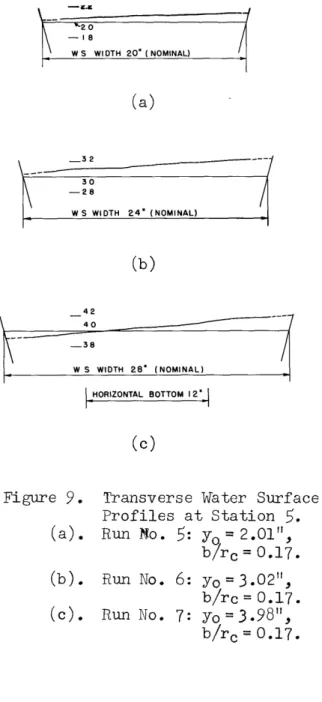
9. Transverse Water Surface Profiles, Station

5,

5,

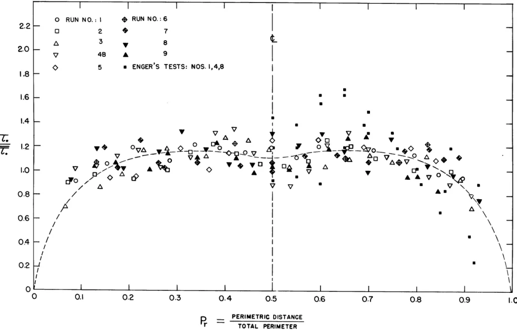
10. Peripheral Distribution of Boundary Shear in Straight 36 Trapezoidal Channels

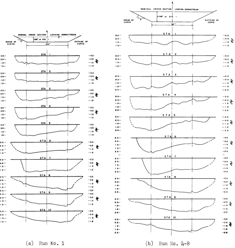
11. Boundary Shear Contour Map: Run No. 1 37 12. Boundary Shear Contour Map: Run No. 2 38 13. Boundary Shear Contour Map: Run No. 3 39

14. Boundary Shear Contour Map: Run No. 4

40

5

16. Boundary Shear Contour Map: Run No. 6 42

17. Boundary Shear Contour Map: Run No. 7 43

18. Velocity Distributions: Run No. 9

47

19. Transverse Water Surface Profiles: Run No. 9 47

20. Boundary Shear Contour Map: Run No. 8 49 21. Boundary Shear Contour Map: Run No. 9

50

22. Velocity and Shear Distributions in the Approach Flow:

53

23. Velocity and Shear Distributions in the Approach Flow:

53

24. Velocity and Shear Distributions in the Approach Flow:

53

25. Velocity and Shear Distributions in the Approach Flow:

53

-viii-Figure _Page

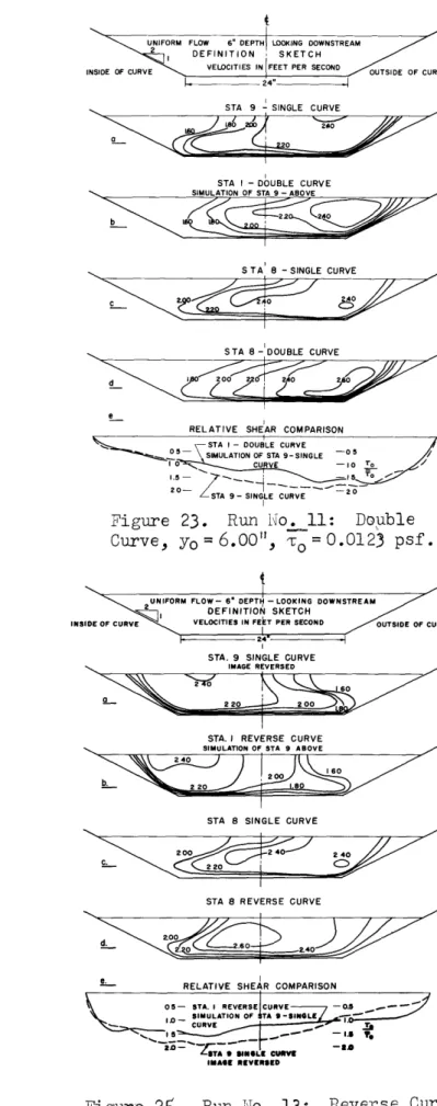
26. Transverse Water Surface Profiles: Run No. 11

₅₄

27. _{Transverse Water Surface Profiles: Run No. 13}

₅₄

₅₇

30. Boundary Shear Contour Map: Run No. 12

₅₉

31. Boundary Shear Contour Map: Run No. 13 60

32. Plot of Computed Maximum Superelevation 68 33. _{Shear Distribution by Sections: Runs No. 1 and h-B 75}

34.

Runs No. 1 and 4-b

35. _{Variation with Curvature of the Total Mean Shear Stress 78} 36. _{Variation with Curvature of the Maximum Relative Shear 78}

37. _{Variation with Curvature of Scour Areas 79}

38. Map and Sections of an Alluvial Stream 85

APPENDIX

A-1 _{General Plan of Experimental Facility 99}

A-2 Overall View of Channel ₁₀₀

A-3 Instrument Carriage Mounted in the Curve 100

A-4 _{Baffle Screen Arrangement for Simulated Curve 101}

A-5 _{Surface Drag Screen used in Curve Simulation 101}

A-6 _{Pitot Tube for Measuring Velocities near the Wall 103}

A-7 Model II Surface Pitot Tube ₁₀₃

A-8 Micromanome ter

₁₀₄

A-9 Development of the Inclined Yanometer ₁₀₄

A-10 Inclined Manometer ₁₀₄

A-ll _{Velocity Distribution above the Smooth Test Surface 121} A-12 _{The Simplified Preston Calibration Curve 121}

A-13 _{Velocity Distribution above the Rough Test Surface 122}

A-lh _{Surface Pitot Tube Calibration, Rough Boundary 122}

-ix-DEFINITIONS AND NOTATIONS

A M channel cross-section area.

b a bottom width of channel.

Cfx _{a mean coefficient of friction at section s n X/}

d _{a diameter of Pitot and Prandtl tubes.}

IF * Froude Number a V/ 6 .

g = gravitational acceleration, ft/sec'.

H₀ * specific Head, yo +V;,/2g, ft-lb/lb.

AH * manometer reading, f t. of water.

k - absolute height of roughness particle.

ks - equivalent sand roughness height.

L = centerline arc length of the test reach.

pt - total, or stagnation pressure, lb/ft.

po - static pressure, lb/ft2 .

P - wetted perimeter.

Q m volumetric rate of flow, fta/sec. r M radial distance to a point in curve.

rc = radius of curvature of channel centerline.

ro _{radius of curvature of outer edge of water surface.} R = hydraulic radius, A/P, f t.

IR M Reynolds number, bRV/v.

Ex Boundary layer Reynolds Number Vx/v. R,% Shear Reynolds number, u,y/v.

So channel slope, ft/ft.

Se n energy gradient ft/ft.

Sex * local rate of energy dissipation at section x, ft-lb/lb/ft.

T

=

u,v * local velocity, ft/sec.

u* - shear velocity,

VTOp,

V a free stream velocity or average velocity, Q/A, ft/sec. w a water surface width.

x W longitudinal distance measured along channel centerline. y = distance normal to plane of channel bottom.

ym - average depth - A/w.

70o total depth of flow. z = transverse distance.

a - angular misalignment of test probe. y -- specific weight of liquid, lb/ft3

S - boundary layer thickness, ft.

9 = local central angle of curvature from beginning of bend, degrees.

= dynamic viscosity of fluid, lb-sec/fta.

v a kinematic viscosity of fluid, ft2_/sec.

p - mass density of fluid, slugs/fta

T 0 a local boundary shear stress, lb/ft4.

O - averaLe boundary shear stress at curve entrance (Sta.11)lb/ft2

.

Tx - average boundary shear stress at section x. L

L average boundary shear stress over the full test reach.

f(),() function of.

i-I. INTRODUCTION

Stream meandering has become a problem of real economic importance in recent years as the amount of valuable land destroyed by bank erosion steadily increases. In large, navigable streams, meandering must be corrected and controlled by costly dredging, and by construction of revetments. The amount of agricultural land lost due to erosion by

smaller alluvial streams can hardly be estimated, but its extent has stimulated an increasing amount of research in this field. The immediate

practical interest has been in developing methods to stabilize the

streams and so to prevent further progression of the meanders.

For lack of systematic quantitative information on the modes of

erosion in curves, the installation of revetments has an empirical basis, founded upon field studies of localized stream systems (36)(42). The success of these revetment projects has been so varied that it is still

not possible to design stabilization works with assurance. In general, the cost of stabilizing small alluvial streams is in excess of

$50,000

with time. It is quite common to find several feet of alluvium deposited over new revetments in an area which had formerly been undergoing active erosion.

A great deal of effort has been devoted to the general study of

stream hydraulics and stream morphology (24)(27)(28)(43). Laboratory

studics (13)(26), have resulted in further understanding of the geometry

of meander patterns in alluvial streams. These investigations give a fairly good indication to the engineer of what to expect in the way of

meander patterns and downvalley progression of bands, but they do not supply him with adequate information to control these phenomena. In addition, studies of velocity distributions in bends (31)(39) have been

useful in gaining a clearer conception of the dynamics of stream flow through crxves, but they fail to delineate the extent and degree of attack on the stream bed. A flowing stream dissipates its energy through shear or tractive forces on its boundaries. For an alluvial stream which is

free from obstructions and major irregularities, erosion and movement of bed material will be controlled by this boundary shear stress and the

current pattern. The shear stress parameter has long been used in the

definition of stability of straight channels and has been extensively studied (10)(22)(25). For such a channel the average shear stress can

be computed reasonably well from a coefficient of resistance and the mean

velocity head. Within a curved reach however, the local shear stresses

vary in a manner which cannot be predicted at present due to the effects

of local accelerations and of secondary motion in the flow.

It is recognized that to completely divorce the problem of

erosion from the related problems of deposition and sediment transport

is, in the final analysis, unrealistic. Not only do all three factors

appear to be integral aspects of the continuously variable phenomenon of

sediment mechanics, _{but there is also compelling evidence that the presence}

of suspended particles modifies the dynaric properties of the transporting fluid (3)(9)(45). However, the quantitative understanding of these latter

phenomena is still a very distant goal, and an experimental attack on the whole problem would not permit at present a clear cut separation of the

various influences inherent in this problem. For this reason a limited

excluded, the channel geometry remains clearly defined and only the effect of the flow pattern on the boundary is determined.

The experimental phase of the investigation consists of a series of tests conducted in curving trapezoidal channels. For fixed boundary geometries, boundary shear stresses were mapped under varied conditions

of flow. An attempt is made, insofar as possible, to correlate trends in

the shear patterns with variations in flow rate and geometry. Velocity

distributions and water surface configurations were recorded for

assis-tance in developing a more general understanding of curved flow, through which erosive attack in channel boundaries may be anticipated.

It is hoped that ultimately these findings may have practical

value in determining the degree and areal extent of protective works

required to stabilize natural stream channels. The practical applications of this work will be limited to those cases where mean shear stress is a dominant factor in bank stability, such as in streams flowing over sur-faces of relatively uniform texture. The introduction of individual bank protrusions creates yet another problem which is not amenable to treatment

II. FLOW THROUGH CURVED CHANNELS: A REVIEW

As a basic model of flow through channel curves, consider first the flow through a deep, smooth-surfaced, prismatic bend. If frictional

effects are assumed negligible, potential theory permits description of

the curved flow as a free vortex. _{M4ockmore (31), among others, has}

demonstrated that at some distance from the boundaries both the velocity distribution and the transverse water surface profile are well described

by an irrotational vortex. For this case the transverse velocity

dis-tribution is given by the constant product of local tangential velocity, u, and radius, r. _{By equating the radial forces on a fluid particle as,}

"2 U(1)

dr r

the water surface profile can be computed from

AY a1f dr ,(2)

where the flow in the curve is assumed to be concentric. For the free vortex the water surface profile is hyperbolic, convex upward.

However, examination of the flow near the boundaries shows that even in a smooth-walled flume, frictional effects combined with the

superelevation tend to cause two important deviations from potential flow:

helicoidal motion of the main stream and separation in zones of adverse pressure gradient.

In 1876 Thompson (4) gave his now familiar explanation of

helicoidal, or spiral flow as being due to the difference in centripetal

acceleration between the fluid near the bottom, which has been retarded by boundary drag, _{and the faster moving layers near the free surface.}

00f 1'

This acceleration, which results from the radial increase in depth (and hence in pressure) causes the low velocity fluid near the bed to move

towards the center of the curve, while the fluid near the surface, having

excess momentum, moves towards the outside.

The superelevation of the water surface in a channel curve leads to two occurrences of longitudinal increase in depth: along the outer

bank of the curve as the water rises entering the curve, and at the curve exit along the inner bank where the flow recovers to normal depth (see for example, Figures

5

kinetic energy to move against a pressure gradient and separation of the boundary layer from the s treambank results. A simple circular curve

connecting two tangent channels is likely to produce larger separation zones than would a natural stream bend, with more gradual transitions. In periods of high flows separation in natural channel bends manifests itself as eddies or "bank rollers" and results in bar deposits.

It has been pointed out (26)(46) that superelevation as such in subcritical, curving flow is quite insensitive to radial variation in the velocity distribution. Substitution into Equation (2) of other assumed velocity distributions, and integration over the full width of the stream, gives only minor variations in the total elevation difference, even though the surface profiles vary in shape. Superelevation is a result of curved flow for all fluids, and is essentially independent of

the frictional aspects and the velocity distribution of the flow. It is

controlled primarily by the boundary geometry and the mean momentum of

separation and helicoid motion take place, their direct cause is boundary friction or shear stress, and in a completely frictionless flow they could

not occur.

In deep, turbulent streams, the separation zone at the concave

bank is usually obliterated by the turbulent infusion of momentum from

the main body of the stream, although bank rollers are observed at the outside of abrupt, shallow bends. The separation zone at the inner bank is more persistent, as shown by the point bar deposits common to virtually all streams except those which are deeply incised and actively degrading.

The persistence and extent of this latter zone is due both to the abrupt

rise in water surface at this point, and to the spiral motion of the stream which tends to move the faster moving fluid to the opposite bank.

Examples of helicoidal motion and separation in a laboratory flume

bend are shown in Figures 1 and 2. Both of these photographs were taken

from the bend exit, facing upstream, so that the flow is from top to

bottom of the photographs. Figure 1 was taken after dye had been injected

and allowed to spread to the full extent of the separation zones. In

Figure 2 the fainter dark streaks were caused by dye crystals moving towards the inner bank with the bottom current (the dashed arrow) while the heavier plume was made by continuous injection of dye at the surface, (the solid arrow).

These two phenomena have far reaching effects on the flow in

natural streams. The helicoidal pattern is, perhaps, the more important, in that, by shifting the faster moving fluid to the outside of the bend, it tends to suppress the free vortex pattern. Einstein and Harder (8) show experimentally that, for a curve of sufficient length, a stable velocity distribution develops in which the velocity increases radially

0007

outwards. That is, of course, the phenomenon observed in long river curves in which the thalweg remains near to the concave bank.

The pattern of helicoidal flows in the bend of a rectangular flume was studied by Shukry (39) using a Pitot sphere to determine the three components of the local velocity vector. It was found that the

helicoidal (i.e. radial) velocities increase with increasing relative

curvature, w/rc and ratio of width to depth, w/y,. Einstein and

Harder (8) also observed that increasing the ratio, w/y0, as well as

increasing the boundary roughness, led to high velocities towards the outer bank, due, presumably, to a more pronounced helicoidal motion.

The laboratory bends in which the irrotational type of flow is

observed are too short to complete the transfer of the filament of

highest velocity to the outer bank. The patterns of flow in sharp bends

-- of both flumes and rivers -- represent a transitional type which, with

sufficient length of curved reach, would develop into the friction

con-trolled flow described above. The length of this transition reach,

however, has not been well defined in terms of the pertinent parameters.

Recently Leopold and co-workers (26) have reported an investi-gation on the frictional resistance of rigid sinuous channels. By

studying the overall head loss over a reach, for channels of constant shape but varied sinuosities, the authors show that not only is the total energy dissipation greater in curved channels than in straight, but that it increases discontinuously above a certain threshold Froude number, due

to the formation of local standing waves, or "spills", along the banks.

While the rate of increase in total boundary shear is not clearly defined, a relationship is suggested between the ratio of width to radius and the Froude number at which the discontinuity occurs. In the laboratory tests

the threshold Froude number varied from about 0.h to 0.6, while, from a

survey of river data, the authors found that bankfull flows generally

occur in streams in the range 0.2 < F < 0.45. They suggest that the rare occurrence of higher Froude numbers may be due to a tendency of alluvial rivers to eliminate local areas of high resistance. Such a

local reduction in boundary shear could come about through erosion of the banks at points of greatest spill occurence, where there is increased dissipation of energy.

The relationship between shear stresses and erosion is further

complicated in natural streams by loose bed material which permits an

additional degree of freedom not possessed by rigid boundary flumes. This freedom to shape its own bed undoubtedly causes a river to alter its flow pattern in ways which cannot readily be predicted from a study of

rigid, prismatic channels (23). Thus, scour will occur in regions of

high shear stress; the modifica.tions in the bed configuration caused by the scour will in turn modify the current pattern and hence the shear distribution.

Previous investigations of energy dissipation in curved flow have been restricted to one-dimensional analyses for both open and enclosed

conduits. As shown by Anderson (2), the different experimental techniques, as well as the varied definitions of a loss coefficient, used by past

investigators have led to considerable confusion. Ito (21) has

demon-strated, by a re-analysis of early data, that the loss coefficient of a smooth bend can be predicted empirically, if the measurements and defi-nitions are given a common basis. With respect to the present study, a

one-dimensional approach is not very revealing in that it gives no indication as to the distribution of the boundary shear stresses which

cause the loss in bends. Indeed, as is shown in the discussion to follow,

the mean section loss gives little indication of the magnitudes of the

local shears, and that the location and intensity of erosive attack cannot be predicted by this means.

III. EXPERIMENTAL EQUIPNFNT AND TECHNIQUES A. The Test Channel

1. Description of the Equipment

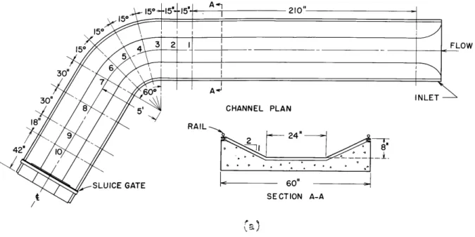
The experiments were conducted in the two trapezoidal flumes shown

in Figure _{3. In both channels the general arrangement is the same,}

consisting of a straight approach section 20 feet in length, a single curve of 60 degree central angle, and a straight 10 foot exit section. The side slopes are constant at 2 horizontal to 1 vertical and the

channels were constructed with the invert horizontal along all radial

sections. _{A smooth entrance transition from the stilling basin at the} upstream end of the approach channel reduces the tendencies for local separation. _{Additional control of depth is provided by an adjustable} sluice gate mounted at the exit section. Details of the basic design of the channel facility are given in Appendix A.

The larger flume (Figure 3a) has a 24-inch base width, and the radius of the curve centerline is 60 inches. For the smaller flume, which was laid in the bed of the larger, the base width dimension was halved, and the stream section was shifted outward to follow the concave bank of the original curve, giving a curve centerline radius of 70 inches.

In a curved trapezoidal stream, the relative curvature -- i.e. the ratio of surface width to bend radius -- varies with depth and thus cannot be given solely in terms of the boundary geometry. However, the limiting values of relative curvature are those set by the base width. Thus, the

range of curvatures which may be obtained in the two flumes is limited by - > _{rc rc} - w 0.0 and - > _{rc rc}- - 0.17 in the larger and smaller channels,

0012

SLUICE GATE GO"

SECTION B-B

Figure 3. The Trapezoidal Channels. The locations of the ten test statione are indicated by the dashed section lines.

moderate range in relative curvature, the lower limit of which is fixed by the boundary curvatures, b

r c

During the installation of the original flumne structure, the centerline slope was set at 0.00064 n 1/1563. The slope was not adjusted throughout the test program; however, after construction of the smaller channel, it was found that the approach slope had decreased to 0.00055 due to settling of the foundations.

The channels were treated with a waterproof plastic coating which dries to form a tough elastic film. For the series of smooth boundary tests it was found that this material provides a hydraulically smooth surface, giving a mean IManning coefficient of 0.010.

For the rough boundary tests which were conducted in the larger

channel the surface was prepared as follows: the channel was given two coats of varnish; while the surface was still wet, roughness particles

were _{spread by hand over the bottom and sidewalls of the section. After}

the material had dried, the surface was scraped with a flat bar to knock off any protruding particles, and then sealed with a final coat of varnish.

The rough surface was applied over 15 feet of the approach section, through

the curve and for 8 feet in the exit reach. The roughness particles are

uniform, rectangular, lucite parallelepipeds, of the approximate dimensions,

0.18 x 0.10 x 0.10 inches. The absolute roughness height of the completed

surface was taken as 0.1 inches; for the treated channel the Manning coefficient is 0.017.

Aodification of the test facility to incorporate additional

combinations of curves would have entailed great additional expense. Therefore, the effects of varied channel alignment were studied through simulation of the flow disturbances caused by curvature in the approach

channel. For this purpose, sets of screen baffles were installed in the upstream tangent. The different screen combinations were established by

trial and error to produce the desired flow patterns at the entrance to

the curve. A typical screen arrangement is shown in Figures A-4 and A-5, Appendix A.

2. Operating Conditions

For each desired depth condition, the discharge at uniform flow

was calculated from the Manning equation. During the early tests in the

smooth channels the Manning coefficient was assumed as n = 0.009. As

the test program continued the channel resistance could be checked, and

it was found that the proper value for the plastic finish was n = 0.010.

A similar trial procedure in the rough channel gave the Manning coefficient,

n

=

With the proper discharge flowing in the channel, the sluice gate was employed to adjust the depth at the entrance to the curve. This downstream control was necessary because of the backwater effects of the

channel outfall which, before its installation, had been observed to extend through the curve and well into the approach tangent.

Flow uniformity had little significance in the tests on the

simulated curve systems due to the large scale modification of the flow

pattern produced by the screens. For these tests, therefore, the

dis-charges and sluice gate settings were those established for the corres-ponding tests at uniform approach condition.

B. Instrumentation

1. The Measurement of Boundary Shear Stress

a. General Requirements: The basic objective of this study

involved the mapping of boundary shear intensities in the curved test

reach at varied conditions of flow. Thus, the primary requirements of the shear instrument to be used were that it be readily movable and that it have a rapid response.

Because of the secondary currents in the bend region, it was

further necessary that the instrument be insensitive to moderate variations in the direction of flow. Local velocities close to the boundary in a bend possess lateral as well as longitudinal components, and consequently the boundary shear stresses are also skewed with respect the the channel centerline. _{For moderate skewness however (e.g. less than 20 degrees),} the magnitudes of the local velocities and boundary shear stresses may be taken as equal to their downstream components. Thus, local shear

magnitudes may be adequately determined with an instrument aligned parallel to the downstream direction, provided the instrument itself is not subject to appreciable error arising from lateral components of flow.

A discussion of methods of determining local shears is given in

Appendix C; each of the techniques listed was reviewed in terms of the

requirements of this study.

b. Shear Measuremen by Surface Pitot Tubes: Of the various

means available for the measurement of boundary shear stress the surface Pitot tube technique developed by Preston (37) was found to be best suited

to the purposes of this study. By this method, the shear stress on a

( IM I I

Pitot tube resting on the surface. Preston demonstrated that, for a tube

of sufficiently large diameter, the effects of the viscous sublayer become negligible, and the mean total pressure over the face of the tube is dependent only on the velocity distribution in the turbulent boundary layer.

The velocity distribution in the turbulent boundary layer over a smooth surface can be expressed,

u _{-- f(-} (* y _{U - - (3)}

u* vp

Preston developed the functional groupings by which the shear stress at

the wall, T,, could be expressed as a dependent variable, and by direct

calibration in pipe flows obtained the equation,

,0d2 (pt-p )da

log - - 1.396 + 0.875 log (4)

hpva 4pv2

valid within the range,

4.5

_{< 6.5.}

Here p and v are the density and kinematic viscosity of the fluid, and

(pt-p,) is the dynamic pressure recorded by a round Pitot tube of outer diameter a d. This calibration equation depends on the velocity distri-bution near the wall which was found to be expressible as the power law,

u _- U*y

8.*61 (-) ₍₅₎

u, v

Although Preston developed Equation

(4)

ratio of inner to outer diameters, Hsu (18) later showed, both analytically and by experiment, that, for a tube of given outer diameter, the internal

diameter has negligible effect on the Pitot tube calibration.

Equation (4) was verified by both Preston and Hsu on flat surfaces

under varied pressure gradients. For the present open channel work, the

calibration was first checked directly in a tilting glass flume. In the

curve of the trapezoidal test channel, however, direct calibration was not possible because of the non-uniformity of the flow. In order to

establish the validity of Equation (4) for this application, velocity

profiles in the flow immediately adjacent to the boundary (y < 1 cm) were

taken at various points in the curve. By this method the existence of

the velocity distribution given by Equation (5) was established (see

Figure A-ll, Appendix D); therefore, the validity of Equation (h) could

be assumed, subject to the restriction that the surface Pitot tube lie wholly within the established boundary layer region of similarity.

For the rough boundary tests, a surface Pitot calibration was developed, which had been suggested in principle by Preston. In

turbulent flow over a hydraulically rough surface, the velocity

distri-bution being _{independent of Reynolds number may be expressed,}

- fa) , (6)

u* ak

where k is the absolute height of the boundary protrusions. Thus, by dimensional considerations alone, the expression analogous to Equation (h)

becomes,

(pt-p = fbP

A8I

direct application of Equation (7) would be questionable, due to the

uncertainty of consistent Pitot tube placement. Furthermore, from

analysis of Nikuradse's rough surface velocity data (33), it seems clear

that f., in EquatIon (7), should vary with the value of y0/k.

If, however, tests are conducted over a limited range of y,/k on a surface of sufficiently uniform roughness, then it should be possible

to find a single form of Equation (7). Direct calibration of a round Pitot tube was performed in a tilting flume on an artificially roughened surface, identical to that which was later used in the test channel.

The test conditions were: d = 0.432", k - 0.1", 2"< y0 < 6", for mean

velocities ranging up to

5

- 0.021 (pyPo), (8)

is valid only for the above set of conditions. Since the calibration

was performed with only one Pitot tube, the general dimensionless expression, Equation (7), was not established, and the restricted form, Equation (8), is to be preferred.

An extended discussion of the principles underlying the use of

surface Pitot tubes, together with calibration procedures is presented in Appendix D.

c. Experimental Application: (i) Smooth Surface. Various models of surface Pitot tubes, which are described in Appendix B, were employed during the tests. The final version, designated as the Model III

instrument, is shown in Figure

h.

0019

(a.) Instrument Mounted on Flat Surface.

TOTAL HEAD TUBE

STATIC TOTAL A TUBE SOLDER A-A FILLET

0.028" DIA. - 2 EAC14 SIDE

0.125" O.D.

0.090" 1. D. ST. STEEL WITH HEMISPHERICAL TIP

TEFLON

0.25" O.D.

0.18" I.D. ST. STEEL TUBE

2n:trvc ion. d~etil shoing the slere -ylir1erical at-he Figure 4. Model III Surface Pitot Tube

ez-i

U-assembly of the instrument it was determined that the two tubes exert no mutual interference, and that the pressurein the channel curve is

hydrostatically distributed over the depth- of flow. The two leads from the instrument are connected to a manometer to give the desired dynamic

head, (pt-p,)/y.

To measure the boundary shear stress at a paint, the instrument

is mounted vertically with the total head tube aligned parallel to the downstream direction and the tip resting on the boundary. The shear

value is computed from Equation (4) using the dynamic head as read from

a manometer. _{Because each test involved about 200 readings, it was} expedient to re-arrange and plot Equation (4) _{to give a direct graphical}

solution of to. (See Figure A-12, Appendix D).

In preliminary tests it was found that the instrument is quite insensitive to moderate misalignment of the probe axis with the local

direction of velocity. For deflection angles up to 200, the error in

measured shear stress varies essentially as (1-cos a); at a - 200 the

error is 60 , and at a - 150 the error is about 30,6. Dye traces in

the channel curve _{revealed a maximum angularity of the flow of about 200,}

which is confined however to a very thin zone adjacent to the boundary. (ii) Rough Surface. For the measurement of shear stress on the rough test surface, the Model III tube was fitted with the adapter sleeve and bushing shown in Figure 4 which raised the diameter of the impact tube to 0.432 inches. This was done in order to increase the value of the manometer readings obtained, as well as to reduce the effects of local

disturbances due to the individualroughness particles. The procedure for

measuring shear stress with the modified instrument is essentially the same as the smooth surface technique, the value of to being computed in

0021

this case from Equation (8).

2. Additional Instrumentation

a. Pressure Jeasurements: Pressures were measured with the two manometers described in Appendix B and shown in Figures A-8 and A-10. The manometers could in general be used interchangeably, depending on the range and precision required. The inclined manometer, being the

faster and more convenient of the two, was used in most of the work. The micromanometer was necessary to measure head differentials outside of the range offthe inclined manometer and for those cases where absolute pressures were required.

b. Depth Measurements: Depths of water in the channel were

measured with a point gauge mounted on the instrument carriage. Ine certain of the tests it was more convenient to determine depths from static

pressure measurements which were correlated with the centerline depths as determined from the point gauge readings.

c. Velocity Measurements: Stream velocities were measured with a

5/16-inch

urn

002

IV. THE EXPERIMENTAL PROGRAi

A. Scope of the Study

The tests were conducted in the two channels shown in Figures 3a and 3b, covering the range of flow geometries which is summarized in Tables I and II.

With the exception of Runs 10-13, the flow entering the curve was essentially uniform and symmetrical about the centerline. For purposes of discussion, therefore, it is convenient to consider Runs 1-9 as

comprising one test series covering a broad range of boundary geometries

for the simple configuration of a curve with straight tangents. Runs 1-7 comprise the complete series of smoothsurface, single curve tests;

for Runs 8 and 9, the channel roughness was increased' and flows were studied for stream geometries similar to those in Runs 2 and

h.

In Runs 10-13, the velocity distribution in the approach flow was modified through installation of various combinations of baffle screens. By superposing asymmetrical conditions on the entrance flow it was possible to simulate the effects of varied upstream channel alignments. Tests at two depths were conducted to determine the shear pattern in a

sequent bend of a double series (U>-configuration), and a reverse series (3-configuration) of curves.

During the course of the test series various modifications were made in the design of the surface Pitot tube. The classification of

instrument models, as listed in Table II, is given with a description of

the instruments in Appendix B. In order to establish that the measured

distributions of relative shear were not influenced by the specific model designs, the shear measurements were completely re-taken with

TABLE I

Summary of Channel Geometries Covered in the Test Program.

Nominal Stream Dimensions w w YO _{r c} Channel Dimensions 12 0.60 10 0.67 b/re = 0'40 8.8 0.73 Fig. 3a 8 0.80 10 0.29 8 0.34 b/rc = 0.17 7 0.40 Fig. 3b 10 0.67 8 0.80 10 0.67 Sb/r = 0.4o 8 0.80 Fig. 3a 10 0.67 8 0.80 Boundary Roughness Velocity Distribution in Approach Flow Smooth n = 0.010 Rough n = 0.017 Smooth n = 0.010 Symmetric; Single curve with straight tangents. Asymmetric; Flow pattern modified to simulate up-stream curvature. Run No.

41- -1

TABLE II

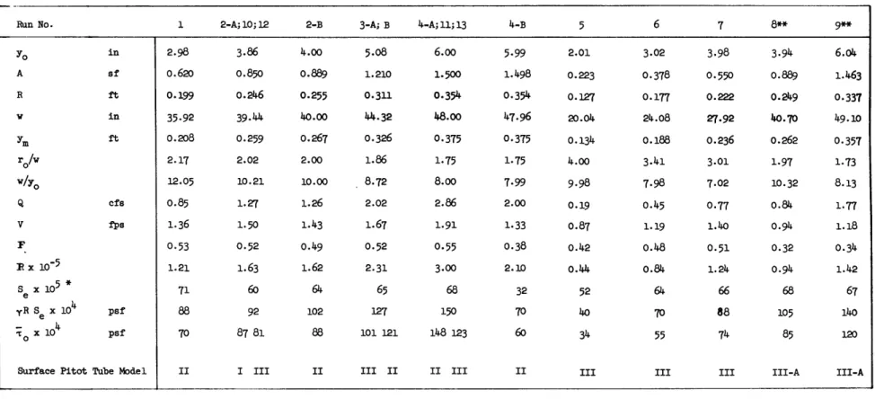
Summary of Test Conditions Determined in the Approach Flow (Station 1).

Run No. 1 2-A;10;12 2-B 3-A; B 4-A;l1;13 4-B 5 6 7 8** 9**

YO in 2.98 3.86 4.oo 5.08 6.oo 5.99 2.01 3.02 3.98 3.94 6.04 A sf 0.620 0.850 0.889 1.210 1-500 1.498 0.223 0-378 0.550 0.889 1.463 R ft 0.199 0.246 0.255 0-311 0-354 0.354 0.127 0.177 0.222 0.249 0.337 w in 35-92 39-44 40.oo 44-32 48.00 47.96 20.04 24.08 27.92 40.70 49.10 ym ft o.208 0.259 0.267 0.326 0.375 0.375 0.134 0.188 0.236 0.262 0.357 r0/w 2.17 2.02 2.00 1.86 1.75 1-75 4.00 3.41 3.01 1.97 1.73 w/yo 12.05 10.21 10.00 8.72 8.00 7.99 9.98 7.98 7.02 10.32 8.13

Q efs o.85 1.27 1.26 2.02 2.86 2.00 0.19 0.45 0.77 o.84 1.77

V fps 1.36 1.50 1.43 1.67 1.91 1.33 0.87 1.19 1.40 0.94 1.18 F 0.53 0.52 o.49 0.52 0.55 0.38 o.42 0.48 0.51 0.32 0.34 R x 10- 1.21 1.63 1.62 2.31 3.00 2.10 o.44 o.84 1.24 0.94 1.42 S x 105* 71 60 64 65 68 32 52 64 66 68 67 yR S, x 104 psf 88 92 102 127 150 70 40 70 88 105 140 ;x 104 psf 70 87 81 88 101 121 148 123 60 34 55 74 85 120

Surface Pitot Tube Model II I III II III II II III II III III III III-A III-A

*The bottom slope, So, is assumed as 0.00064 in all but Runs 5-7; in Runs 5, 6, 7, So 0.00055.

different instruments. Comparison of the shear distributions for Run2-A (Model I) with 2-B (Model II), and _{Run 3-A (Model III) with 3-B (Model II),} showed that, while the absolute magnitudes of the local shears varied with

the model used, there were no essential differences in the maps of

rela-tive shear given in _{terms of the mean shear stress measured at Station 1,}

To.

In performing the runs on the simulated curve systems with the Model III tube, it was simply necessary, on the basis of the above tests,

to re-measure the shear distribution at Station 1 and then to apply the

relative shear data as computed previously. Thus the second value of

T given in Table II for Run 2-A and for Run h-A, represents the

measure-ment with the Model III instrumeasure-ment, which was used in the corresponding

compound crwe tests.

It will also be noticed that while two tests were conducted at a

6 inch depth, the energy gradient, mean velocity, and hence the shear

stress of the approach flow were varied markedly between the two runs. Unlike Runs 2 and 3 which were repeated at similar conditions in order to verify the experimental techniques, Runs h-A and -B represent essentially

different tests. The purpose of these tests, which are discussed in a

later section, was to study the effect of approach flow non-uniformity on the shear pattern in the curve.

For all of the tests boundary shear stresses were measured at the

ten test stations indicated in Figures 3a and 3b. Highly non-uniform

shear patterns in several of the runs made it necessary to add two inter-mediate sections between Stations 7 and 8. Shear measurements were taken at 2" intervals across each station, covering the full wetted perimeter except the outer 4" along each side.

velocities were made at each station in Runs

1-4.

It should be mentioned that the numbering system of the test

runs shown in Table I was established to give a logical sequence to the

order of discussion, and that it does not follow the chronological order of the experiments. All of the tests involving the larger smooth channel

(Figure 3a) were completed before application of the rough surface. Following the completion of the two tests on the rough surface, the channel was modified to give the flume arrangement shown in Figure 3b, and the final three tests were those conducted in the smaller smooth surfaced channel.

B. Presentation of Data

The volume of the basic data compiled during the course of this study is such that direct presentation of the tubulated material would

make analysis difficult. Therefore, in order to facilitate the dis-cussions of the results, the data presented herein have been reduced to graphical form. The complete compilation of tabulated data has been printed and is available in the basic data supplements of Hydrodynamics Laboratory Technical Report No.

43

47

The data figures for the various tests are presented in the

appropriate discussion sections in the following text. Before proceeding

with the discussions, however, it is convenient to define the method of U

-presentation of each group of data.

1. Velocity and Water Surface Profile Data.

The velocity distributions and transverse surface profiles are presented by stream sections following the sequence of test stations in

the curved reach. Because of the repetitive nature of these patterns drawings were prepared only for representative tests.

2. Boundary Shear Stress Data.

The value of the mean measured shear stress at Station 1, om,

was determined for each test by graphical integration of a plot of the local shear stress, 'To, over the wetted perimeter;

dP] ₍₉₎

P ~Sta.l1

The maps of boundary shear distributin for the full test series are

presented in terms of relative local shear, - / '0. This form is

preferable to reporting absolute values, since application of the results

is simpler, and the shear patterns for varying flow conditions are readily

compared. The absolute magnitudes of local shears may be computed from

the shear maps using the values of 7~ (Table I) obtained from Equation (9). 0

V. DISCUSSION OF RESULTS

A. Tests Conducted with Uniform Conditions of Approach: Flow Through

Single Curves

1. Smooth Channel, Runs 1-7.

a. Entrance Conditions. For the series of tests conducted in the smooth

channels with undisturbed approach conditions, the velocity, water surface

and shear stress configurations at the entrance to the test section are essentially summetrical about the centerline axis (Figures 5-10). At conditions of greater relative curvature and depth a slight asymmetry becomes evident at Station 1 due to the backwater effects of the curve. It seems clear however that the flow pattern in the bend cannot be ascribed to upstream distortion of the flow.

The existence of a fully developed turbulent boundary layer was desired at the entrance to the curve. The boundary layer thickness, 6,

may be approximated by the Blasius expression, assuming turbulent conditions from the channel entrance, x

=

_L - 0.38 ₍₁₀₎

X

(Y-)Y'5

Substitution of the values, V = 1.50 fps and v -

105

6 " 4.6 inches at x - 20 feet. Because of the relatively small variation in Reynolds numbers, the boundary layer thickness varied only a small

amount over the full set of flow conditions. Thus the boundary layer was fully developed in Runs 1-2 and

5-7,

4.

Because the low channel slope made it impossible to obtain the energy gradient accurately, it is not known to what extent fully uniform

V. DISCUSSION OF RESULTS

A. Tests Conducted with Uniform Conditions of Approach: Flow Through

Single Curves

1. Smooth Channel, Runs 1-7.

a. Entrance Conditions. For the series of tests conducted in the smooth channels with undisturbed approach conditions, the velocity, water surface and shear stress configurations at the entrance to the test section are essentially summetrical about the centerline axis (Figures

5-10).

It seems clear however that the flow pattern in the bend cannot be ascribed to upstream distortion of the flow.

The existence of a fully developed turbulent boundary layer was

desired at the entrance to the curve. The boundary layer thickness, 6,

may be approximated by the Blasius expression, assuming turbulent

conditions from the channel entrance, x

= 0;

0.38 (10)

V

Substitution of the values, V - 1.50 fps and v -

10-5

6- 4-6

in Reynolds numbers, the boundary layer thickness varied only a small amount over the full set of flow conditions. Thus the boundary layer was

fully developed in Runs 1-2 and

_5-7,

and 6-inch depths, Runs 3 and

4.

Because the low channel slope made it impossible to obtain the energy gradient accurately, it is not known to what extent fully uniform

flow was achieved. However, it is believed that this condition is not of great consequence for the results of this study. It will be noted that Runs h-A and B represent the largest variation in F and Se, yet the

contours of uo/ -r for these tests were found to be virtually identical.

Thus, while the magnitude of the mean shear stress varies essentially as the mean velocity head, the distribution of relative shears is but

little affected by variations in the Froude number and energy gradient

of the approach flow.

b. Flow through the Curve. The flow through the channel bend exhibits

the expected tendency towards free vortex motion, and in the upstream

portion of the curve (Stations

3-5)

surface configurations are in general agreement with those found by

previous investigatbrs (31)(39). For the full range of conditions

tested the maximum total water surface superelevations (See Section V-'

below) as well as the surface profile shapes (Figures 8 and 9) conform

quite closely to the trend predictable for free vortices.

The irrotational aspects of the flow are most pronounced at

conditions of greatest depth and curvature. In Runs 1-4, the irrotational type of motion persists over the full length of the curve, and high

velocities appear along the outer bank only at the start of the downstream

tangent. (Figures

5

5,

Attention is called here once move to the phenomenon previously discussed which are not readily apparent form the plots of velocities and surface elevation: separation and helicoidal motion.

Figures

5,

Channel.

Figure 5. Run No. 1.

yO - 2.98", w/y - 12, w/re O.6

Figure 6. Run No. h-B.

yom 5.99', w/y-8, w/r-O.8

Figure 7. Run No. 6.

YO - 3.02, w/y. - 8, w/r. - O.34.

K - W~ -- 0-tft

2 DEFINITION SKETCH

INSIDESCF 2 96 VELOCTE S N FEET OUTSIDE OF PERV SECOD CURVE

LOORING DOWNSTREAM VERTICAL SCALE MAGNIFICATION 2X 24 STA I S TA 2 STA 3 STA 4 sepin STA 5 1700 STA 6 16 1 40 I130 septn _{STA 7} 614 I30 STA 8 +-170 14 0 ISO 16 0 140 50 0 STAI 10 0io 170)

130

15

SS* VELOCITIES IN FEET PER SEC INSIDE OF 'I LOOKINd. DOWNSTREAM OTSIDE OF

CURVE 24" CURVE STA I I150 I1O 140 I5O STA 2 130 140 STA 3 I160-~ 30 SA4

sep'n

302 VELOCITIES IN FEET PER SEC INS I DE OF LOOKING'DOWNSTREAM OUTSIDE OF CURVE 12 _ _CURVE STA I S3 STA 4 STA 5 14 3I I-SA 60 1 4 STA 7 STA. 8 5,6,7 STA 3 10-1 11