Applying network coding to TCP

ARCHPuvwS

Applying Network Coding to TCP

Leonardo Andres Urbina Tovar

Submitted to the Department of Electrical Engineering and Computer Science

in partial fulfillment of the requirements for the degree of

Master of Engineering in Electrical Engineering and Computer Science at the

MASSACHUSETTS INSTITUTE OF TECHNOLOGY

June 2012

@

in whole or in part.

A uthor ... ...

Department o i trical Engineering and Computer Science May 25, 2012 Certified by ... ...

.

....

Muriel Medard Professor of Electrical Engineering Thesis Supervisor Certified by. ... Minji Kim Postdoctoral Associate Thesis Supervisor Accepted by ... Dennis Freeman Chairman, Department Committee on Graduate Theses

Applying Network Coding to TCP by

Leonardo Andres Urbina Tovar

Submitted to the Department of Electrical Engineering and Computer Science on May 25, 2012, in partial fulfillment of the

requirements for the degree of

Master of Engineering in Electrical Engineering and Computer Science

Abstract

In this thesis, I contribute to the design and implemention of a new TCP-like proto-col, CTCP, that uses network coding to provide better network use of the network bandwidth in a wireless environment. CTCP provides the same guarantees as TCP whilst providing significant enhancements to previous TCP implementations, such as permitting multipath packet delivery. CTCP's flow and congestion control policies are based on those of TCP Reno and TCP Vegas, which allow for prompt recovery from packet erasures and cope with congested networks. Unlike previous attempts at using network coding with TCP, this implementation uses block coding schemes, which are better suited to delay sensitive applications. As a result, CTCP permits content streaming. Overall, the efficient integration of network coding into CTCP allows for improved robustness against erasures as well as efficient content delivery over multiple paths.

Thesis Supervisor: Muriel M6dard Title: Professor of Electrical Engineering

Thesis Supervisor: Minji Kim Title: Postdoctoral Associate

Acknowledgments

This work would have not been possible without the support from several people. First and foremost, I would like to thank both my parents. My mother, Aury, for her unconditional love and her wise advise. My father, Wilfredo, who served as an inspiration to me since I was a very young boy, introducing me to the world of Mathematics and always finding ways to show me its beauty.

I would like to thank my advisor, professor Muriel M6dard, for her support, pa-tience, trust and respect. Specifically, she served served a crucial role in providing theoretical insights that helped shape the overall system. Also, Minji Kim's support, guidance and patience throughout the project was indispensable for its culmination. I would also like to thank Megumi Ando. She was a pillar of support and helped in every aspect to be able to complete this work. She was always there for me, from brainstorming, to helping with correction, to making me caffeinated tea late into the night. Thank you.

Finally, I would like to thank other people that helped in the completion of this project such as Ali Parendegheibi Parandehgheibi, David Foss and Sukru Cinar.

Contents

3 System Design & Implementation

3.1 Efficient Network Coding Integration ... 3.1.1 Banded Matrices ...

3.1.2 Dynamic Coding Window ...

3.1.3 Gaussian Elimination ...

3.1.4 Expected Completion Time ... 3.1.5 Other Optimizations ...

3.2 Delay Sensitive Applications ... 3.3 End to End Behavior ...

3.3.1 CTCP Server ...

3.3.2 CTCP Client . . . .

3.3.3 CTCP at the Packet and Block levels . 3.4 Flow and Congestion Control . . . . 3.4.1 Congestion Control . . . . 15 16 17 19 19 21 21 23 . . . . 24 . . . . 25 . . . . 26 . . . . 26 . . . . 29 . . . . 32 . . . . 32 . . . . 34 . . . . 35 . . . . 36 . . . . 37 . . . . 38 . . . . 38

3.4.2 Flow Control and Erasure Detection . . . . 39 3.5 Multiple Hardware Interfaces . . . . 40 3.5.1 Issues with Asymmetric Connections . . . . 40

4 Results 43 4.1 Single Interface . . . . 43 4.2 Multiple Interfaces . . . . 45 5 Conclusions 51 5.1 Future W ork . . . . 51 A Graphs 53

B List of Data Structures 69

C Inverse of Banded Matrices 73

D CTCP Source Snippets 87

D.1 CTCP Server . . . . 87 D.2 CTCP Client . . . . 90

File subdivision into blocks and segments . . . .

Main components of CTCP client/server application. . . . .

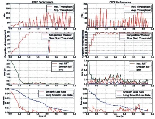
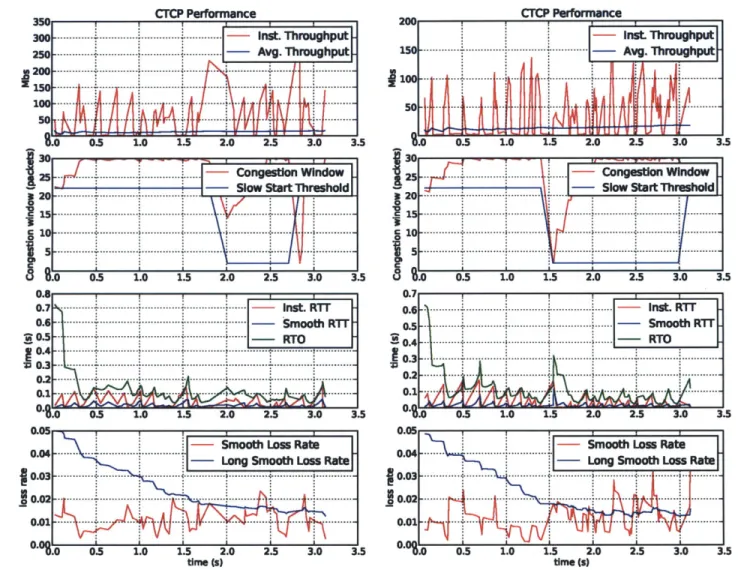
4-1 TCP connection with 5% added loss rate .. . . . . 4-2 CTCP performance with 5% added loss rate. Top to bottom: 1)

Instan-taneous throughput (red), average throughput (green); 2) congestion window (blue stars), ssthresh (red); 3) RTO (green), instant rtt (red), srtt (blue); 4) smooth loss rate (red) and long smooth loss rate (blue). 4-3 CTCP using two USB wireless antennas with 0% added loss rate. 4-4 CTCP using two USB wireless antennas with 5% added loss rate. 4-5 CTCP using two USB wireless antennas with

4-6 CTCP using two USB wireless antennas with

A-1 TCP connection with 0% added A-2 TCP connection with 1% added A-3 TCP connection with 2% added A-4 TCP connection with 5% added A-5 Single interface CTCP with 0% A-6 Single interface CTCP with 1% A-7 Single interface CTCP with 2% A-8 Single interface CTCP with 5% A-9 Single interface CTCP with 0% A-10 Single interface CTCP with 1% A-11 Single interface CTCP with 2%

loss rate. . loss rate. . loss rate. . loss rate. . added loss added loss added loss added loss added loss added loss added loss

10% added loss rate. 15% added loss rate..

33 34 44 45 47 48 49 50 . . . . 54 . . . . 55 . . . . 56 . . . . 57 rate . . . . 58 rate . . . . 59 rate . . . . 60 rate . . . . 61 rate . . . . 62 rate . . . . 63 rate . . . . 64

List of Figures

A-12 Single interface CTCP with 5% added loss rate A-13 Single interface CTCP with 7% added loss rate A-14 Single interface CTCP with 10% added loss rate A-15 Single interface CTCP with 15% added loss rate C-1 Sparsity histogram for n = 64, bandwidth = 1 C-2 Sparsity histogram for n = 64, bandwidth = 3 C-3 Sparsity histogram for n = 64, bandwidth = 5 C-4 Sparsity histogram for n = 64, bandwidth = 7 C-5 Sparsity histogram for n = 128, bandwidth = 1 C-6 Sparsity histogram for n = 128, bandwidth = 3

C-7 Sparsity histogram for n = 128, bandwidth = 5

C-8 Sparsity histogram for n = 128, bandwidth = 7 C-9 Sparsity histogram for n = 256, bandwidth = 1 C-10 Sparsity histogram for n = 256, bandwidth = 3

C-11 Sparsity histogram for n = 256, bandwidth = 5

C-12 Sparsity histogram for n = 256, bandwidth = 7

C-13 Sparsity histogram for n = 512, bandwidth = 1 C-14 Sparsity histogram for n = 512, bandwidth = 3 C-15 Sparsity histogram for n = 512, bandwidth = 5 C-16 Sparsity histogram for n = 512, bandwidth = 7 C-17 Sparsity histogram for n = 512, bandwidth = 9 C-18 Sparsity histogram for n = 1024, bandwidth = 1

C-19 Sparsity histogram for n = 1024, bandwidth = 3 C-20 Sparsity histogram for n = 1024, bandwidth = 5 C-21 Sparsity histogram for n = 1024, bandwidth = 7 C-22 Sparsity histogram for n = 1024, bandwidth = 9

65 . . . . 6 6 . . . . 6 7 . . . . 6 8 . . . . 75 . . . . 75 . . . . 76 . . . . 76 . . . . 7 7 . . . . 7 7 . . . . 78 . . . . 78 . . . . 79 . . . . 79 . . . . 8 0 . . . . 8 0 . . . . 8 1 . . . . 8 1 . . . . 8 2 . . . . 8 2 . . . . 8 3 . . . . 8 3 . . . . 84 . . . . 84 . . . . 8 5 85

List of Tables

List of Algorithms

1 Insert(x ,p): . . . . 28

Chapter 1

Introduction

The Transmission Control Protocol (TCP) [2] is one of the core protocols used for networked communications and is part of the Internet Protocol Suite, the other mem-ber being the Internet Protocol (IP). These two protocols combined conform what is generally referred to as the TCP/IP stack. The main functionality of TCP is to offer

a connection oriented stream delivery service for application programs, providing the following: reliable in order delivery of data packets, error detection, flow control and congestion control.

TCP was originally designed in 1974, and since then it has undergone several revisions. It is to be noticed, however, that heuristics used in the congestion control algorithms in TCP were designed with wired networks in mind. For example: (1) TCP regards any evidence of lost data as congestion in the network, and (2) TCP can only communicate with one hardware interface at a time.

Regarding (1), TCP will, when there is evidence of data loss, decrease the rate at which the data is being sent. While this behavior is appropriate in wired networks, in wireless networks lossiness can be due to other factors, such as node mobility and background noise. Regarding (2), TCP was developed without the notion of mobile devices and pervasive wireless data networks as we have today. Back then, a single hardware connection would suffice to include a computer in a network, and thus TCP was designed around this model. A modern desktop, laptop or mobile device will have several hardware interfaces to connect to different networks, including wireless

and cellular data networks. Owing to the way TCP is currently implemented, it is not possible for a connection to use more than one interface at a time.

With this in mind, we are faced with modern mobile devices that use TCP in order to interface with wireless networks. However, given the aforementioned assumptions on which TCP is based, these devices perform sub-optimally in terms of bandwidth usage with connections that are very fragile in lossy environments.

In recent years researchers have attempted to solve these issues by developing new protocols that are capable of multipath packet delivery to improve both perfor-mance and robustness in the aforementioned scenarios [19, 15, 20]. Most notably, the development of a "Multi-Path TCP" (MPTCP) has been proposed and and sev-eral specifications have been drafted. To date, the implementations of this protocol remain limited to simulations, and research seems to have stagnated since 2009.

In this work we have chosen a different path. We use a technique known as network coding to aid us develop a TCP like protocol that addresses the aforementioned challenges.

1.1

Related Work

Network coding was originally developed by Ahlswede et al. [1] in 2000. Ever since, its theoretical properties, such as better bandwidth utilization and increased robustness in lossy networks, have sparked interest into using this technique in transport proto-cols [17, 18, 13]. However, the functionality of current implementations of network protocols integrating network coding have proved limited.

The work by Sundarajaan et al. [17, 18] proposes a TCP like protocol integrating network coding. However, it uses a sliding window approach for coding operations can have significant decoding delay and may have undesirable worst case behavior. In addition it still requires an implementation in the kernel. In a similar fashion, the work by Liu et al. [13] develops a real world implementation of a transport protocol that integrates network coding for content streaming. However, the protocol proves to be very computationally expensive and thus not suited for devices with limited

computational power, such as mobile phones.

1.2

Contributions

In this work, I design and implement a new TCP-like protocol, CTCP, that inte-grates network coding to provide better network utilization and increased robustness in lossy environments. CTCP, unlike previous attempts at integrating network coding with TCP, supports delay sensitive applications, such as content streaming. More-over, CTCP supports multipath packet delivery using multiple hardware interfaces, further increasing the robustness and performance of connections. Finally, by using a novel technique we develop that we refer Sparse Network Coding, we were able integrate network coding into CTCP while minimizing the additional computational overhead. To demonstrate our design we have implemented an application layer ver-sion of CTCP.

Chapter 2

Preliminaries

2.1

Network Coding

The theoretical advantages of network coding have been well established in the re-search community in recent years. The works by Ahlswede et al. [1], Koetter et al. [11] and Ho et al. [10], among others, expose network coding as a technique that allows networked communications to have better bandwidth utilization, and increased ro-bustness and loss resiliency. These results have motivated new protocol designs and implementations, including the work by Sundarajan et al. [17, 18], and the work by Liu et al. [13]. Our work follows this trend, tapping into the power of network coding to provide better networking protocols. Before delving into the details of our imple-mentation of network coding we outline the basics of random linear network coding

(RLNC) [10].

Assume that a node is to transfer a data block D over the network. First, it divides the block into n segments D = [S1, S2, . .. , Sn]T, where each segment has

length L bits. The node constructs n coded packets to send across the network by computing payloads [P1, P2,..., P,], each of which is a random linear combination of the segments that make up D. More specifically, each segment is interpreted as a vector of symbols over the field GF(2q), where q consecutive bits make up one symbol.' Unless otherwise stated, all of the operations hereon take place over GF(2q)

for some appropriate q. The payload P is constructed by randomly selecting coding coefficients Ci = [c4,, ... , ci], and computing

n

Pi = Ci -D= E (ck - S).

k=1

Each coded packet consists of a payload P, coding coefficients Ci and additional matadata. Upon receipt of n linearly independent packets, we refer to each of these as a degree of

freedom,

C₁ C2 -- -c S1 P SS _{2 P2} (2.1) cy c -n-- c"Sn- Pn-Or simply, C-Dz=P, (2.2)

where C = [C1, C2, ... , Cn]T and P =[P1, P2, ... -, Pn]T. By using Gaussian elimina-tion the receiver can solve this system, yielding:

D = C- - P (2.3)

and thus recovering the original data. Having understood the basis network coding, it is important to discuss the benefits of using NC to judge when it is best to apply it.

value proves convenient as each byte makes up one symbol over GF(28

). Moreover, this choice of q has been predicted to provide energy efficiency advantages when compared to other possible field

2.1.1

Advantages of Network Coding

Rateless Erasure Codes

Random linear codes are near-optimal rateless erasure codes. Namely, it is possible to generate potentially infinitely many coded packets given a finite set of segments contained in a block of data D. Moreover, given any set of n or greater coded packets, it is possible to decode D with high probability. This is true as the linear equations used to generate the payloads are linearly independent with high probability. Once

n degrees of freedom arrive at the receiver, the original data block will be decodable.

In case of channel erasures, the sender only needs to construct as many packets as those lost and resend these. With high probability, the additional packets will be linearly independent with the packets sent thus far, and therefore be helpful towards the completion of the overall data transfer.

Near-Perfect Asynchronous Coordination

As we stated previously, upon the arrival of n degrees of freedom the original data D becomes decodable. The described scheme is oblivious to the source where the degrees of freedom originated. Hence, an arbitrary number of senders serving the same data D could be used to independently produce the necessary degrees of freedom to complete a data transfer. The latter is done asynchronously, as the payloads generated at each of these sources are linearly independent with high probability, and no synchronization is needed between the different sources for this property to hold. Our implementation takes advantage of this property to allow for delivery of packets using multiple hardware interfaces. This aspect of our implementation is discussed in more depth in Section 3.5. For more details see [5, 10, 14].

2.1.2

Disadvantages of Network Coding

The advantages of network coding come at a price. In particular, the necessary dot and matrix products computed over GF(2q) may be of significant computational cost. This has lead researches to attempt alleviating the computational burden of

network coding using several different types of optimizations. Some of these include architecture specific implementations of the dot and matrix products over GF(24) [8], as well as carefully choosing the parameters involved in the specific protocols [3, 13].

Chapter 3

System Design & Implementation

As mentioned already, the use of network coding allows for better bandwidth use over lossy channels, making networked communications more robust and loss resilient, as well as opening the possibility for packet delivery using multiple hardware interfaces [1, 10, 11, 12, 17]. In this chapter, we describe the design and implementation of CTCP: a novel TCP-like protocol that uses network coding for data transfer in the form of a client-server file transfer application.

CTCP's architecture is driven by three main design objectives: 1) efficient network coding integration, 2) delay sensitive applications such as content streaming and, 3) multipath packet delivery through multiple hardware interfaces. Furthermore, CTCP's implementation preserves the TCP guarantees of error-free, in order delivery of data along with comparable flow and congestion control policies.

The rest of this chapter is organized as follows: Section 3.1 describes how network coding is integrated into CTCP; in particular we describe Sparse Network Coding (SNC), a novel method to reduce the computational complexity of network coding for real world implementations. Section 3.2 describes the design decisions and imple-mentation details that enable content streaming with CTCP. Section 3.3 describes the main components of our implementation of CTCP and their end-to-end behav-ior during a generic file transfer. The policies and recovery systems added to make network coding work smoothly are discussed. Finally, Section 3.4 discusses the flow and congestion control policies implemented in CTCP and how these relate previous

TCP implementations.

Throughout this chapter we refer to the CTCP components by their name in our implementation. Please refer to Appendix B for a complete list of the components' names and descriptions.

3.1

Efficient Network Coding Integration

One of the main challenges of integrating network coding in a real system is the added overhead required for coding and decoding. This added overhead is particularly prob-lematic for the deployment of such systems on mobile devices. Several attempts have been made to alleviate this, including parallelized implementations of the product over GF(2q) for q = 8 for the use on GPGPUs [16],as well as implementing this product using a lookup table approach, among others [3].

During the development of CTCP, we devised a new scheme that we call Sparse

Network Coding (SNC) which allows us to increase the overall performance of the

protocol by decreasing the overhead of coding and decoding when possible, adapting to the estimated channel loss rate. In what follows we describe the details of SNC.

As seen in Section 2.1, a node using RLNC will construct coded packets by com-puting random linear combinations of the segments of the data being served, and subsequently send these to a receiver. The receiver upon receipt will progressively construct and solve a system of linear equations of the form of Equation 2.2, namely:

C-D=P

where D = [S1, S2, ... , Sn]T denotes the data being served and its subdivision into

seg-ments Si, P = [P₁, P2, ... , Pn]T denotes the payloads sent, and C = [C1, C2,... Cn]T,

where Ci denotes the coefficients used to construct the coded packet P.

SNC is a heuristic designed specifically to reduce the decoding overhead of RLNC at the receiver by restricting the way in which the coding coefficients Ci are chosen at the sender. This effectively constrains the set of possible C matrices which need to be

inverted to decode a given data block. Specifically, we want to reduce the number of entries that need to be computed in order to find C-'. Note that standard Gaussian elimination has 0(n3_{) time complexity.}

One way to accomplish this would be to place restrictions so that both C and C are sparse. There are examples of families of sparse matrices whose inverses are also sparse, including nonsingular block-partitioned matrices, as well matrices describing the kinematics and static equations of deformable bodies [6, 9]. However, in our scenario we want to generate the desired matrices randomly, thus the aforementioned families of matrices prove too narrow for our purposes.

3.1.1 Banded Matrices

Instead, SNC uses a different family of sparse matrices called banded matrices. A banded matrix is defined as a sparse matrix whose non-zero entries lie near the diago-nal. As such, we can define the bandwidth of a banded matrix as the smallest number of adjacent diagonals among which the non-zero elements are confined. Following our discussion in the previous section, SNC shall tighten the constraints over C and C-1 so as to make C banded and C sparse. The reasoning is that, assuming C is banded, we can implement a more efficient Gaussian elimination process tailored for this type of matrix. Furthermore, if C-1 is also sparse with roughly 0(n) non-zero entries, then the Gaussian elimination process can be performed in approximately

0(n 2), as only 0(n) entries need to be computed to find the inverse, and each entry

takes 0(n) computations to be found.

The main idea behind SNC is based on the following empirical finding: If C is a banded matrix with small bandwidth (roughly 0(log n)) then C' is sparse with high probability. Hence it suffices to restrict C to a banded matrix. This can be easily accomplished by restricting the way the Ci's are chosen. Namely, we choose these so that they consist of at most k consecutive non-zero coefficients, and zeros elsewhere. In other words, each coded packet is constructed by computing a random linear combination of at most k consecutive segments. For this reason, we refer to k as the coding window, and abbreviate it as coding-wnd. In particular, we notice that

the family of matrices we construct can have their rows rearranged to have bandwidth coding.wnd. This is easily done by placing the set of coefficients with the first non-zero entry at position i in row i. For details on the empirical data please refer to Appendix C.

3.1.2

Dynamic Coding Window

One of the interesting properties of SNC is that it exposes the tradeoff between the computational overhead and robustness against erasures. Namely, if we let coding-wnd equal n (the number of segments), we are left with RLNC. Such a scheme is very robust against erasures, but with computational overhead. At the other end of the spectrum we can set coding-wnd to 1, in which case each coded packet sent is a "random" linear combination of a single segment. This case is almost equivalent to no coding whatsoever as each coded packet consists simply of a single segment multi-plied by a random coefficient.' Hence, this scheme has negligible overhead, however it is almost equivalent to traditional TCP, and thus it losses all of the theoretical advantages of random linear network coding.

Having tradeoff between throughput performance and decoding complexity in mind, we can use SNC in an adaptive fashion: We can tune coding-wnd according to the perceived erasure rate of the channel thus adding only the minimum overhead necessary to achieve the desired amount of robustness. The optimal coding-wnd val-ues for each different erasure levels were found via empirical measures made in our

CTCP implementation as well as Monte Carlo simulations of CTCP.

3.1.3

Gaussian Elimination

SNC guarantees that the rows of coefficients received for a given data block D can be arranged so that they form a banded matrix C. Based on this assumption we designed a Gaussian elimination process tailored to find the inverses of the resulting banded 'For efficiency reasons our implementation of CTCP chooses the first non-zero coefficient of every

Ci to be 1. This avoids the receiver having to normalize each vector when doing Gaussian elimination,

while being equivalent to randomly choosing all of the coefficients. In the case described, setting codingwnd to 1 is equivalent to coding with a permutation matrix.

matrices. Most notably, our Gaussian elimination process is optimistic, namely, it will only perform computations to find the non-zero entries of the inverse. Hence, the time complexity of our algorithm is a function on the number of non-zero entries of the inverse. This fact, combined with the empirical data in Appendix C confirming that the inverse of a random low bandwidth matrix is sparse with high probability, implies that our Gaussian elimination process has time complexity 0(n 2) with high

probability. In what follows we describe this process in detail.

For simplicity, we assume throughout this section that the erasure rate does not dramatically change during the time that it takes to transfer a single data block. Namely, we can assume that coding.wnd is constant throughout the transfer of a given data block D. Also, our implementation of SNC sets the first non-zero coefficient of every Ci vector to 1. This avoids having to normalize the coding vectors at every step of the Gaussian elimination process.

We start out with an empty matrix C and an empty vector P. Our goal is to construct successively C and P, based on contents of the received coded packets. In constructing C, we maintain the following invariant:

Invariant. Every row of C has its first non-zero coefficient in the diagonal and is equal to 1.

All operations performed on C are mirrored on P as well. Once we are done, we are left with a n x n upper triangular matrix C, with all of its diagonal entries equal to 1, and a vector P of payloads that satisfy equation 2.1.

For each Data.pckt that arrives let x = packet-coeff = [X₁, ... , ,z] denote the coefficients used to construct the arriving packet and let p denote the packet's payload. We execute Insert(x,p), which returns a boolean value indicating whether the row was successfully inserted or not. The pseudocode is show below in Algorithm

1:

Lines 1-5 attempt to to place x so that its first non-zero coefficient falls in the diagonal of C. If this is not possible we go to line 7. If j = n, we have reached the end of the matrix and return f alse. Otherwise we continue in line 8, which sets x

Algorithm 1 Insert(x, p):

1:

j

3: Insert x into CUJ

4: Insert p into P[j] 5: Return true 6: else 7: if j < n then 8: x <-x- C[j] 9: X xj+1 10: p p - PU] 11: p + zj+1 12: if x 0 then 13: return Insert( 14: end if 15: end if 16: return false 17: end if x,p)

to the difference between the current j-th row of C and x, and normalizes the result. Given our invariant, we know that the first non-zero entry of x is now in the

j

position, and it equals 1. Line 9 mirrors these operations on the payload. Finally, line 10 places a recursive call to insert the new values of x and p into the

j

After receiving n degrees of freedom, where n is the number of segments that make up the block D, performing the steps above yields:

C - D = P, (3.1)

where C is the desired upper triangular matrix with all of its diagonal entries equal to

1, and it is banded with bandwidth coding-wnd. Finishing the Gaussian elimination

by successively subtracting an appropriate multiple of row k - 1 from row k, for

k = n, n - 1,--- , 2. This is done for both C and P. Once done, we are left with:

I, - D = C-' - P. (3.2)

In other words, the value of D is now stored in the vector where we originally stored the coded payloads. This yields the decoded values that the receiver wanted to obtain in the first place.

3.1.4 Expected Completion Time

In what follows we provide upper an lower bounds for the expected completion time of the overall process of constructing C and P based on the random generation of packets of SNC, and performing Gaussian elimination over them. We focus on the stochastic aspect of this process, while ignoring channel erasures. We start with the upper bounds. Consider the following lemma:

Lemma 1. Assume we have received k degrees of freedom. The probability that a new packet chosen by SNC is a degree of freedom is at least n-k

Proof. If the packets is such that Insert(x, p) would attempt to insert its coefficients

in one of the n - k rows that have not yet been filled, then we are guaranteed for it to be a new degree of freedom. It follows that the probability of being a new degree

of freedom must be at least ". 0

n

With this lemma in mind we proceed by proving the following theorem.

Theorem 1. Using SNC, the expected number of packets that need to be received in order to construct a full rank matrix is bounded above by n(y + ln(n)), where - ~ 0.5772 denotes the Euler-Mascheroni constant.

Proof. After receiving k degrees of freedom we know by lemma 1 that the probability

of receiving a new degree of freedom is at least "-* . Being a geometrically distributed event, the expected number of packets that need to be generated until this happens

is at most n-k. Hence the total number of packets generated until obtaining a full

rank matrix is bounded by:

n-1 n

n - k = n ~ n(-y + ln(n))

k=0 k=1

The result follows.

With this in mind we introduce the following definition.

Definition. Coding Loss Rate: Rate at which linearly dependent packets are

gener-ated. These packets are redundant with previous packets received and thus do not contribute to the overall completion of the data transfer session.

With this notion, from theorem 1 we know that using SNC the coding loss rate is bounded by -y + ln(n). In particular, our implementation uses n = 128. Thus the

coding loss rate is at most ~ 5.3%.

We now proceed to prove lower bounds on the expected completion time of SNC. We do so by assuming that the packets rows of coefficients chosen by SNC are uniform over the space of all possible rows. Consider the following lemma:

Lemma 2. Let V be an n-dimensional vector space over a finite field F and W c V

be a k-dimensional subspace. Also, let M = |Fl. The probability that x, uniformly chosen from V, belongs to W equals Mk-n.

Proof. Let w₁, w2, ... , wk be a basis for W. We can extend it to w₁i, w2, ... k,

Tk+1, ... , rn so that it is a basis of V. Changing basis, we can now view every element

of v E V represented as a vector [01, 2, .... , an]. The event that v E W is equivalent to the event that a, = 0 for

j

equals M = Mk-n.

With this we can prove the following theorem.

Theorem 2. The expected number of packets that need to be generated to obtain a

Proof. After receiving k degrees of freedom we know by lemma 2 the probability that

a newly generated packet will be linearly independent with the previous k degrees of freedom is at most 1- Mk-n. Hence the event of getting the k+ 1-st degree of freedom is geometrically distributed, and thus the expected number of packets that need to be generated until we get the k + 1-st degree of freedom is at least (1 - Mk-n)-1.

Hence, the total number of packets that we need to generate until we obtain a full rank matrix is:

n-1 n-1 1 - Mk-n M--k - 1 k=O k=O n-1 =n ₊ Mn-k - 1 k=O > n.

Since the number of packets is an integer, we conclude that the number of packets must be greater than or equal to n

+

Having these bounds we now consider the Gaussian elimination process.

Theorem 3. The SNC Gaussian elimination has complexity 0(n2) in the best case

and O(n21 nn) in the worst case.

Proof. In the best case, by theorem 2 we know that the total number of packets

generated is O(n). For each packet that arrives, inserting it requires looking at

O(n) rows of the current matrix, where each row has coding-wnd entries. Thus,

constructing the C takes 0(n2_{) operations. C contains O(n) non-zero off-diagonal}

entries. Hence we need O(n) extra operations to finish the process. It follows that the total number of operations needed is O(n2 + n) = 0(n2). The proof for the worst

case is analogous, except we use the bound shown in theorem 1. 0

This is a significant improvement from the 0(n') time of the standard implemen-tation of Gaussian elimination.

3.1.5 Other Optimizations

From the analysis shown in Section 3.1.4, the process of accumulating n degrees of freedom is in the worst case just like coupon collector problem. Namely, at each step the probability of receiving a new degree of freedom, after having received k, equals

n k. Hence, the expected amount of rows that need to be generated until we find

the next degree of freedom is n. As k increases, we spend increasingly more time waiting to get the next degree of freedom.

To cope with this situation, we implemented two heuristics that help us improve the performance of CTCP under most circumstances. The first heuristic consists on forcing the first n packets being sent to be n degrees of freedom. We can guarantee this by making the indices of the position of their first non-zero entries to be a permutation of the numbers 1, 2,... , n. Hence, if there are no erasures, the receiver will be able

to decode the block D after the first n packets arrive, and thus avoids the problems of decreasing probability of success that arise in the coupon collector. Moreover, this systematic approach to coding ensures that the Gaussian elimination will complete in 0(n 2_{) time.}

The other heuristic comes into play once the number of degrees of freedom received exceeds a certain threshold and there has been at least one erasure. In this scenario the sender will emit packets each doubling the value of coding-wnd from the previous. This exponential increase of codingwnd will make sure that we will receive the final degrees of freedom after a constant (small) number of packets have been received. We note, however, that this will marginally increase the overhead of decoding, but it is a cost that we are willing to pay.

3.2

Delay Sensitive Applications

Previous protocol implementations that integrate network coding in their design, in-cluding the work by Sundarajaan et al. [17, 18], Shojnia et al. [8] and Liu et al. [13], compute linear combinations of data chunks across the whole content being transmit-ted. As a result, these protocols are not well-suited for delay sensitive applications,

such as content streaming, as the data received may be undecodable until enough degrees of freedom are received to decode the entire data.

Unlike previous implementations CTCP divides the data to be transferred into two hierarchical subdivisions: blocks and segments. Each block consists of BLOCKSIZE segments, where BLOCKSIZE is a configurable constant. For our purposes this con-stant is set to 128. Each segment is designed to fit (including the CTCP headers) inside a UDP packet without being fragmented by lower layers. For this to hold, we need the CTCP to be within the network MTU. With our network settings it sufficed to set the segment size to 1325 bytes, padded with NULLs if necessary, to account for EOFs.

segment

b2 b3 .. bn

block

Figure 3-1: File subdivision into blocks and segments

To address the issue of streaming we use network coding at the block level. Thus the sender only mixes together segments from the same block and the receiver decodes blocks one by one. As soon as enough degrees of freedom are available to decode a particular block, it is decoded and written to disk. The size of each block, given that each segment is 1341 bytes and BLOCKSIZE is 128, is 167.625 KB making each block reasonably small for the purposes of streaming, permitting content to be buffered.

However, it is worth noting that addressing the content streaming problem while using network coding is not as simple as just splitting a file into blocks and subse-quently into segments. One of the main caveats of such design is block transition: When should the sender stop sending packets of the current block and proceed with the next one while using the available bandwidth efficiently. This issue, along with the strategy used in our implementation are discussed in further detail in Section 3.3.3.

3.3 End to End Behavior

The CTCP implementation follows the client-server pattern, and is done as a file transfer application. The implementation works as a userspace application that uses UDP as the underlying communication protocol. All of the features, including the TCP guarantees, are implemented at the application layer. We chose to implement CTCP in userspace as to avoid directly modifying the kernel's protocol stack and, thus, avoid kernel recompiles among other hassles that this kind of development usually entails. This allowed for rapid prototyping, testing and development and gave us a test bed to understand the effects of policy and feature changes would have on the performance and guarantees of CTCP. The main components of the application are depicted in Figure 3-2 below:

ContmIer

Packet Genrator

Figure 3-2: Main components of CTCP client/server application.

In what follows we describe the end-to-end end behavior of the CTCP client-server application. We start by individually examining the server and the client in sections Section 3.3.1 and Section 3.3.2, respectively. We describe each of their components, the state that they keep, and the procedures that each of them carry out during a generic file transfer session. Finally, in Section 3.3.3, we proceed by looking at the lifespan of an individual DataPckt (our implementation of a coded packet) during a file transfer, as well as describing a file transfer at the block and multi-block level, including block transitions.

3.3.1

CTCP Server

The CTCP server plays the role of the sender in the data transfer sessions. The implementation of the server consists of two main modules: A controller module and a packet generator module. This division allows for all of the IO (e.g. reading from disk), as well as the computations inherent to network coding (e.g. multiplication over GF(28)), to be executed asynchronously in threads separate from the main execution thread. In this section we describe in detail each of these modules' behavior and how they interact with each other.

Controller Module

The controller module is the core component of the CTCP server. It runs in the main thread of the application and it keeps track of the state of any ongoing data transfer sessions. The controller module listens for any incoming requests, and upon receipt of such, it establishes a connection, sends DataPckts and listens for acknowledge-ment packets. The rate at which DataPckts are sent is mandated by the flow and congestion control policies set in place (see Section 3.4 for details), and it depends on the feedback information received through acknowledgment packets.

At any given time of an ongoing data transfer session, the state kept by con-troller module includes the number of the current and next data block, the number of DataPckts allowed to send at the current time, flow and congestion control variables to detect erasures, and react to congestion (for details see Section 3.4).

Packet Generator Module

The packet generator module is responsible for reading data from disk, performing the block and segment subdivisions, and generating the DataPckts needed by the controller module. It runs asynchronously from the main execution thread via a separate threadpool. The communication between the controller and packet generator modules is done through the Job.q thread-safe blocking deque. When needed, the controller can request new DataPckts to be generated by inserting a Coding_ Job_t

into the Job.q. This request specifies the block from which the new DataPckts should be generated from, the number of packets that should be generated as well as the value of coding window coding.wnd. See Section 3.1 for details of the network coding scheme used.

3.3.2

CTCP Client

The CTCP client serves as the receiver during any data transfer session. The client is responsible for initializing the data transfer sessions, processing any incoming DataPckts, decoding and writing to disk decoded data. Unlike the server, the client handles each connection using a single thread. We chose this design, as opposed to having background threads handling the decoding and 10, to avoid situations in which the client receives packets faster than it can decode and write them. This is often true in high speed networks where the overhead from the decoding and/or writing at the receiver dominates the time taken to perform the data transfer. In what follows we list the responsibilities of the client.

1. Initialize the connection: Being the receiver, the client can request a new files to be delivered by the server. In order to do so, the client sends a packet with the SYN flag on, as well as the name of the file that is requesting. Upon receipt of said packet, the server starts a new data transfer session to send the data corresponding to the requested file.

2. Process incoming DataPckts: As new DataPckts arrive for a given data trans-fer session, the client does two things. First, it uses the coefficients and payload of the DataPckt to perform the first step of the decoding (Section 3.1.3). Sec-ond, the client constructs an AckPckt using the information based on the result from the Gaussian elimination, namely, it indicates to the sender whether the received packet's payload and coefficient resulted in a degree of freedom.

3. Decode and write to disk: Once enough degrees of freedom have been received for a given data block, the client performs the last step of Gauss-Jordan

elim-ination, yielding the decoded data for this block. The decoded data is written to disk, and the data transfer session continues.

3.3.3

CTCP at the Packet and Block levels

All data transfer sessions in CTCP start as a request originating from the client asking a server to deliver a specific set of data. This request is in the form of a ActPckt with the SYN flag set, and specifying the name of the file requested. Upon receipt of this request the server's controller module opens the requested file and submits a Coding_ Jobt to read and generate DataPckts corresponding to the first two data blocks using the appropriate value of coding._wnd. Until successful transfer of a given block, the following steps are repeated:

1. The server's controller module sends as many coded packets as permitted by the congestion window cwnd (not to be confused with coding-wnd.

2. Upon receipt of each packet, the client performs the necessary Gaussian elim-ination steps, and emits an appropriate Ack.pckt, containing the necessary feedback information for the server to update its internal state. This includes information to detect erasures, abide the congestion avoiding policies, and start the block transition process, among other things.

3. Upon receipt of an Ack-pckt, the server performs all the state updates as nec-essary and repeats goes back to step 1.

The latter is done until the block has been transfered successfully.

Block Transition

The subdivision of data into blocks and segments gives rise to the problem of block transition. The problem is the following: What should the server do once it knows that the client has received almost enough degrees of freedom to decode a block, and given that the value of the its congestion window cwnd is greater than the number degrees of freedom needed to finish that block. Sending all cwnd packets towards

the current block will guarantee that the client has enough degrees of freedom to decode. This is very inefficient as only a fraction of cwnd packets will suffice, and the remainder will be redundant packets that won't help towards the overall completion of the data transfer. Furthermore, the transmission of the next block is delayed several round trip times causing a overall slower transfer rate. Instead, we want a strategy that minimizes the waste of bandwidth while handling block transitions.

In our implementation we solve this problem by allowing the transmission of two blocks at a time. Namely, once we have are close to finishing the transmission of a block we enter a transition mode in which the server divides the congestion window into two portions: The first portion of cwnd is the size of the number of degrees of freedom needed to finish the current block, plus an additional x% to account for the coding loss rate (usually x is set to 10). The rest of cwnd is used towards the next block. Once the current block is completed, we exit transition mode and continue the data transfer as usual.

3.4

Flow and Congestion Control

The flow and congestion control policies implemented in CTCP borrows ideas from different implementations of TCP, including Reno [2, 71 and Vegas [4], whenever applicable. In what follows we describe these in detail.

3.4.1 Congestion Control

CTCP inherits its congestion control policies from TCP Vegas. It works as follows: After an acknowledgment arrives at the server, the following quantities are computed.

* rtt: Round trip time of the coded packet received.

" srtt: Smooth round trip time. This is computed in a low-pass filter fashion by using the formula:

Algorithm 2 Compute_ cwnd(rtt, srtt, cwnd, v., V, VA): 1: increment +- 1 2: if vA > vp6 then 3: increment <- 1 4: increment <- -1 5: else 6: if vA > v, then 7: increment <- 0 8: end if 9: end if 10: cwnd+ = increm t 11: return cwnd

Where

#

1

- ::: 0.04

(BLOCK SIZE)

VA: The percentage change of rtt with respect to srtt. This is computed using the formula below:

srtt VA = 1 - __

rtt

We control the size of the congestion window cwnd using vA as a proxy for con-gestion. We attempt to maintain vA in between two desired values, va = 0.05 and v6 = 0.2. There are three possible cases: VA < va, Va VA 5 V and v6 < vA. The

pseudocode for Computecwnd is shown in 2 describing the behavior in each of these cases.

Namely, we increase, decrease or keep congestion window the same depending on whether the percentage change of the instantaneous RTT with respect to the smoothed RTT is above, below or within two chosen thresholds, Va and v,, respec-tively.

3.4.2

Flow Control and Erasure Detection

The two main flow control policies used in CTCP are slow start and a sliding window.

* Slow Start: We slow start implemented following the specifications outlined TCP Reno with no changes made to it. It is used at the beginning of every

connection and after every timeout.

* Sliding Window: CTCP borrows some aspects of the sliding window imple-mentation of TCP Reno. However, as described in Section 2.1.1, network is a rateless erasure code, thus greatly simplifying the logic in its implementation. The reason behind this is that we sure that any n linearly independent packets arrive at the receiver, regardless of which packets are. Hence, we slide the win-dow every time that we receive an ack. The wind6w may be slid by an extra amount in the case that the erasures have been detected.

3.5

Multiple Hardware Interfaces

As mentioned in Section 2.1.1, one attractive property of network coding is its capacity of near-perfect asynchronous coordination. This property allows for data connections to happen over multiple hardware interfaces simultaneously. This is especially at-tractive given the presence of multiple wireless interfaces, including 802.11, 3G, LTE and WiMax, in today's mobile devices. Up until now, these devices use the different wireless interfaces available to them in an exclusive fashion, i.e. only one interface is used at a time.

The experience improvements brought to the end user by a protocol supporting, from the ground up, multiple hardware interfaces are twofold: First, if two (or more) hardware interfaces are connected simultaneously to their respective networks and both have good signal quality, the end user ideally would be able to enjoy (close to) the combined throughput of the connected networks. Second, even if the signal of one of the hardware interfaces fades, all of the ongoing data transfer sessions can proceed through the remaining hardware interface(s) until better reception is available.

3.5.1 Issues with Asymmetric Connections

The current implementation of CTCP supports data transfer sessions over multiple hardware interfaces. However, in a design where data is subdivided into blocks and

segments, and network coding is applied solely at the block level to support delay sensitive applications (Section 3.2), it becomes challenging to effectively utilize the bandwidth provided through connections of varying qualities. In particular, the net-work coding property "nearly perfect asynchronous coordination" holds only at the block level. Specifically, if the connection associated with one of the hardware inter-faces has significantly higher throughput and shorter latency, and assuming that all connections available are being used to deliver packets of the current data block, it is likely that most (if not all) of the needed packets will be delivered by the faster inter-face. Now, packets for the current data block have also been requested through the other interfaces, and many of them may still be en route to the receiver, owing to the higher latencies. By the time these packets arrive, the corresponding data block may have already been decoded and written to disk, effectively wasting the bandwidth used to deliver these packets. As a result of this, it is necessary to develop adaptive

strategies to deal with varying latencies and throughputs of the available connections and utilize the available bandwidth as efficiently as possible. In Section 4.2 we discuss the performance obtained by using multiple hardware interfaces. At this stage CTCP has no policies that allows for better handling of assymetric connections.

Chapter 4

Results

Our testing was performed using off-the-shelf commodity hardware running Ubuntu 10.04. The server machine had an 12-core Intel Core i7 running 3.47GHz with 16GB of RAM. The client machine had an Intel Core i5 running at 3.20GHz with 3GB of RAM. The server machine was directly connected to the internet via an ethernet jack. The client machine was connected to the internet via our campus wide wireless network, via a USB wireless antenna compliant with the 802.11n draft specification. Each experiment consisted in sending an 11MB file over the network and recording performance including the average and instantaneous throughput as well as latency.

In what follows we show the results obtained.

4.1

Single Interface

We were interested in understanding the performance of CTCP as compared to TCP in a lossy environment. In order to have TCP as our baseline, we setup an FTP server to host the same files as the CTCP server. We explicitly avoided scp or any other file transfer tools that rely on encrypted connections, as accounting for the encryption overhead made the performance comparison harder to make.

Owing to the inherent fluctuation of the wireless network signal, we performed CTCP transfers back to back with TCP (using FTP) transfers, assuming that the connectivity would not change drastically between transfers. This was done several

times in order to arrive to what we consider is average behavior of CTCP and TCP over the given networks. Furthermore, in order to guarantee a certain level of losses we used iptables to force a certain percentage of packet loss at the kernel level on the server. The experiments were performed with added loss rates of 0%, 1%, 2% and 5% for both TCP and CTCP. Notice however that we had no control over the background loss rate. Thus we can only guarantee a lower bound on the loss rates. The experiments were performed several times for each added loss rate. The graphs shown were considered to be representative of the average behavior of each protocol. In this section we show and analyze the experiments performed with 5% added loss rate as they best illustrates the advantages of CTCP over TCP. For completeness we have included the rest of the experiment's graphs in Appendix A.

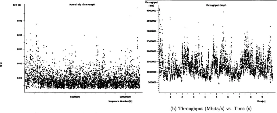
We start by looking at TCP the performance of a TCP connection with 5% added loss rate, as shown in Figure 4-1. The two graphs correspond to the latency and the throughput over time. This connection recorded an average throughput of 9.92Mbit/sec and an average latency of 6ms, lasting a total of 10 seconds.

orr [S] 4ound Sp Timeo Graph

0.040-0.035- -4000000.

0.025- r .9 A1

0.0.S

1000000 102 0S 3 0 7 0 1

s5*90eqn Num4ber(] Times)

(a) Round Trip Time (s) vs. Sequence no. (b) Throughput (Mbits/s) vs. Time (s)

Figure 4-1: TCP connection with 5% added loss rate.

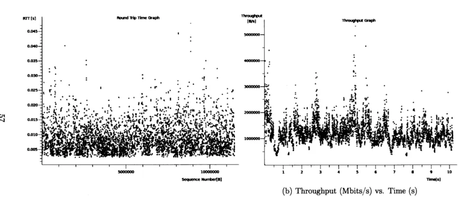
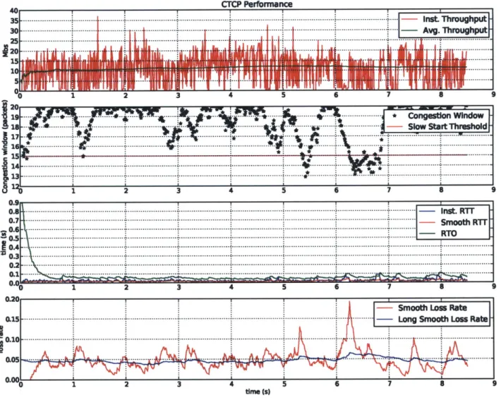
In comparison, Figure 4-2 shows the performance of a CTCP connection with 5% added loss rate. The four graphs following quantities over time, from top to bottom: throughput, congestion window, latency and loss rate. The connection recorded an average throughput of 13.89 Mbits/sec and an average latency of 11ms.

35 cCnu. Ianwindow 30 ... ... ... ... .. ... - ... ... ... .... . - U kW f T1 1 v mu 25~ ~ ... ~ ... .... . ... ...

4...

Figure... 4.2 .T.prorac.ih.%add osr. To tbooM:)Intn

taneous~~~~~~~~~. thrugpu (rd) veae hoghu. (re);2.cnesinwidw.bu stas) ssthres (rd) 3) AN TO (green),. instant r.t.red,.stt.blue;.4.smothlos..

4. Mutil Interfaces

faes We oufte theot .... cletcmue ihtoietclUB lncMplan

wireless... anen a to... test. thi functionalit. We.. repetedl performe th sa..e exper-.. ... iment... of... sending. an 11MB .fI over.. the.. network.. We.esedadedlos.ats.anin

between 0% and 15%. We show graphs for the connections that we considered por-trayed the average behavior of CTCP. In what follows we discuss the performance of connections performed under 0%, 5% and 15% loss rate. We chiefly interested in understanding the performance and robustness gains when using multiple hardware interfaces.

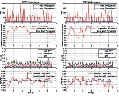
Figure 4-3 below shows the performance of multipath CTCP with 0% added loss rate. The average bandwidth for each of the interfaces were 13.5 Mbits/sec and 16.28 Mbits/sec, respectively. Hence in total we have an effective combined bandwidth of approximately 30 Mbits/sec. The average RTT for each interface were 8ms and 6ms respectively. The average perceived loss rates were 0.18% and 0.48%, respectively. This is a significant increase from the performance that a standard TCP connection could attain using WiFi. It is to note however, that the experiments were performed by connecting both wireless antennas to the same network. Using different networks, or even, different kinds of antennas still proves problematic. In the scenario where the different interfaces are connected to networks with very different latencies, the slower interface tends to not contribute to the overall completion of the transfer, as all the packets it request, by the time they arrive are redundant and thus dropped.

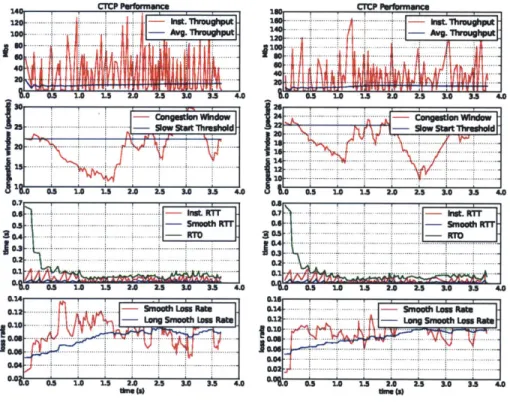
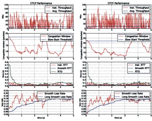
Finally we look at the performance of multipath CTCP in highly noisy environ-ments. Figures 4-4,4-5, 4-6 show the performance of multipath CTCP on channels with 5%, 10% and 15% added loss rate, respectively. This noise level beyond what

TCP can handle. We now look at the performance of each of these connections: For 5% added loss rate (Figure 4-4) the average throughputs were 8.99 Mbits/sec and 9.3 Mbits/sec and the average RTTs were 10ms and 15ms, for each the interfaces respectively. For 10% added loss rate (Figure 4-5) the average throughputs obtained

were 13.79 Mbits/sec and 13.13 Mbits/sec, respectively. This time the average RTTs were 7ms and 6ms. Finally, for 15% added loss rate (Figure 4-6) the average through-puts obtained were 9.89 Mbits/sec and 10.25 Mbits/sec with average RTTs of 5ms and 6ms, for each the interfaces respectively.

Overall we can see that the added robustness in multipath CTCP can handle loss rates that are beyond what TCP can handle, while still performing at very