Strengths and challenges for transient Mid-to Late Holocene simulations with dynamical vegetation

HAL Id: hal-03018647

https://hal.archives-ouvertes.fr/hal-03018647

Submitted on 23 Nov 2020

HAL is a multi-disciplinary open access

archive for the deposit and dissemination of

sci-entific research documents, whether they are

pub-lished or not. The documents may come from

teaching and research institutions in France or

abroad, or from public or private research centers.

L’archive ouverte pluridisciplinaire HAL, est

destinée au dépôt et à la diffusion de documents

scientifiques de niveau recherche, publiés ou non,

émanant des établissements d’enseignement et de

recherche français ou étrangers, des laboratoires

publics ou privés.

https://doi.org/10.5194/cp-15-997-2019

© Author(s) 2019. This work is distributed under the Creative Commons Attribution 4.0 License.

Strengths and challenges for transient Mid- to Late Holocene

simulations with dynamical vegetation

Pascale Braconnot, Dan Zhu, Olivier Marti, and Jérôme Servonnat

IPSL/Laboratoire des Sciences du Climat et de l’Environnement, unité mixte CEA-CNRS-UVSQ, Université Paris Saclay, Bât. 714, Orme de Merisiers, 91191 Gif-sur-Yvette CEDEX, France

Correspondence:Pascale Braconnot (pascale.braconnot@lsce.ipsl.fr) Received: 20 October 2018 – Discussion started: 2 November 2018 Revised: 2 May 2019 – Accepted: 17 May 2019 – Published: 13 June 2019

Abstract. We present the first simulation of the last 6000 years with a version of the IPSL Earth system model that includes interactive dynamical vegetation and carbon cy-cle. It is discussed in the light of a set of Mid-Holocene and preindustrial simulations performed to set up the model ver-sion and to initialize the dynamical vegetation. These sensi-tivity experiments remind us that model quality or realism is not only a function of model parameterizations and tun-ings but also of experimental setup. The transient simulations shows that the long-term trends in temperature and precipita-tion have a similar shape to the insolaprecipita-tion forcing, except at the Equator, at high latitudes, and south of 40◦S. In these re-gions cloud cover, sea ice, snow, or ocean heat content feed-backs lead to smaller or opposite temperature responses. The long-term trend in tree line in the Northern Hemisphere is reproduced and starts earlier than the southward shift in veg-etation over the Sahel. Despite little change in forest cover over Eurasia, a long-term change in forest composition is simulated, including large centennial variability. The rapid increase in atmospheric CO2in the last centuries of the

sim-ulation enhances tree growth and counteracts the long-term trends induced by Holocene insolation in the Northern Hemi-sphere and amplifies it in the Southern HemiHemi-sphere. We also highlight some limits in the evaluation of such a simulation resulting from model climate–vegetation biases, the diffi-culty of fully assessing the result for preindustrial or modern conditions that are affected by land use, and the possibility of multi-vegetation states under modern conditions.

1 Introduction

Past environmental records such as lake levels or pollen records highlight substantial changes in the global vegeta-tion cover during the Holocene (COHMAP-Members, 1988; Wanner et al., 2008). The Early to Mid-Holocene optimum period was characterized by a northward extension of boreal forest over north Eurasia and America, which attests to in-creased temperature in midlatitudes to high latitudes (Pren-tice and Webb, 1998). A massive expansion of moisture and precipitation in Afro-Asian regions has been related to en-hance boreal summer monsoon (Jolly et al., 1998; Lezine et al., 2011). These changes were triggered by latitudinal and seasonal changes in top-of-the-atmosphere (TOA) incoming solar radiation caused by the long-term variation in Earth’s orbital parameters (Berger, 1978). During the course of the Holocene these features retreated towards their modern dis-tribution (Wanner et al., 2008). While global data syntheses exist for the Mid-Holocene (Bartlein et al., 2011; Prentice et al., 2011; Harrison, 2017), reconstructions focus in gen-eral on a location or a region when considering the whole Holocene. For example, regional syntheses for long-term pa-leorecords over Europe reveal long-term vegetation changes that can be attributed to changes in temperature or precip-itation induced by insolation changes (Davis et al., 2003; Mauri et al., 2015). Similarly, over West Africa or Arabia, pollen data suggest a southward retreat of the intertropical convergence zone (Lezine et al., 2017) and a reduction in North African monsoon intensity (Hély et al., 2014). The pace of these changes varies from one region to the other (e.g., Fig. 6.9 in Jansen et al., 2007; Renssen et al., 2012) and has been punctuated by millennium-scale variability or abrupt events (deMenocal et al., 2000), for which it is still

un-indicate, however, that vegetation plays a role in triggering the African monsoon during the Mid-Holocene (Braconnot and Kageyama, 2015) but also that soil moisture might play a larger role than anticipated (Levis et al., 2004). Reduced dust emission with increased vegetation and changed soil properties has been shown to amplify monsoon changes (Albani et al., 2015; Pausata et al., 2016; Egerer et al., 2017). At high latitude as well, the role of the vegetation feedback is not fully understood. Previous studies showed that the response of vegetation in spring combined with the response of the ocean in autumn were key factors to transforming the seasonally varying insolation forcing into an annual mean warming (Wohlfahrt et al., 2004). The magnitude of this feedback has been questioned by Otto et al. (2009), showing that vegetation was mainly responding to the ocean and sea-ice-induced warming over land. The role and magnitude of the vegetation feedback over Asia were also questioned (Dallmeyer et al., 2010). The variety of the responses of dynamical vegetation models to external forcing is an issue in these discussions. However, they all produce increased vegetation in the Sahel when forced with Mid-Holocene boundary conditions, which suggests that, despite large uncertainties, robust basic response can be inferred from current models (Hopcroft et al., 2017). Other studies have highlighted that there might be several possible vegetation distributions at the regional scale for a given climate that can be related to instable vegetation states (e.g., Claussen, 2009). This is still part of the important questions that must be answered to fully explain the end of the African humid period around 4000–5000 BP (Liu et al., 2007).

It is not clear yet that more comprehensive models and long Holocene simulations can help solve all the questions, given all the uncertainties described above. But they can help to solve the question of the vegetation–climate state and of the links between insolation, trace gases, climate, and veg-etation changes at global and regional scales. For this, we investigate the last 6000-year long-term trend and variabil-ity of vegetation characteristics as simulated by a version of the IPSL model with an interactive carbon cycle and dy-namical vegetation. Off-line simulations, using the original scheme for dynamical vegetation of ORCHIDEE, were al-ready used to analyze Mid-Holocene and LGM (Last Glacial

external forcing is applied to the model can also lead to cli-matology or vegetation differences between two simulations with the same model. It is thus important to know how the changes we made to the IPSL climate model to set up the version with dynamical vegetation affect the results and the realisms we can expect from the transient simulations. We thus investigate first how the major changes and tuning af-fect the Mid-Holocene simulations and the performances of the model compared to simulations with the previous model version IPSLCM5A (Dufresne et al., 2013; Kageyama et al., 2013a). Several questions guide the analyses of the transient experiment. Is the long-term response of climate and vege-tation a direct response to the insolation forcing? How large is the impact of the trace gases? How different is the timing of the vegetation change in different regions? Do we need to take into account variability over such a long time period? We also need to put the responses to these questions in per-spective with the level of realism we can expect from the sim-ulated vegetation in such a simulation. It concerns the model biases and the compatibility between the climate and vegeta-tion states produced by the transient simulavegeta-tion or obtained from snapshot experiments. Also, different strategies can be used to initialize the vegetation dynamics and produce the Mid-Holocene initial state for the transient simulation. We investigate if they have an impact on the simulated vegeta-tion distribuvegeta-tion.

The remainder of the paper is organized as follow. Sec-tion 2 describes the experimental setup, the characteristics of the land surface model as well as different model adjust-ments we made and the initial state for the dynamical veg-etation. Section 3 presents the transient simulation focusing on long-term climate and vegetation trends at global and re-gional scales. Section 4 discusses the realism of the simulated vegetation and different sources of uncertainties that can af-fect it before the conclusion is presented in Sect. 5.

2 Model and the suite of experiments

2.1 Experimental design

The Mid-Holocene (MH) time-slice climate experiment (6000 BP) represents the initial state for the last 6000-year

transient simulation with dynamical vegetation. It is thus considered as a reference climate in this study. Because of this, and to save computing time, model adjustments made to set up the model content and the model configuration were mainly done running MH and not preindustrial (PI) simu-lations (Tables 1 and 2). Only a subset of PI simusimu-lations is available for comparison with modern conditions. All the simulations were run long enough (300–1000 years) to reach a radiative equilibrium and be representative of a stabilized MH climate (Fig. 1). They are free of any artificial long-term trends after the adjustment phase, as were IPSL PMIP3 MH simulations (Fig. 1; Kageyama et al., 2013a).

Most tests follow the MH-PMIP3 protocol (Braconnot et al., 2012). This is only due to the fact that this work began before the PMIP4 boundary conditions were available. But the transient simulation (TRHOLV, for TRansient HOLocene simulation with dynamical Vegetation) and the 1000-year-long MH simulations with or without dynamical vegeta-tion that were run to prepare the initial state for it follow the PMIP4-CMIP6 protocol (Otto-Bliesner et al., 2017, Ta-ble 1). In all simulations the Earth’s orbital parameters are derived from Berger (1978). The MH-PMIP3 protocol uses the trace gases (CO2, CH4and N2O) reconstruction from ice

core data by Joos and Spahni (2008). It has been updated for PMIP4, using new data and a revised chronology that provides a consistent history of the evolution of these gases across the Holocene (Otto-Bliesner et al., 2017). The differ-ence in forcing between PMIP4 and PMIP3 was estimated to be −0.8 W m−2by Otto-Bliesner et al. (2017). This is the or-der of magnitude found for the imbalance in net surface heat flux at the beginning of the MH-FPMIP4 simulation. This simulation started from L11Aer run with the PMIP3 proto-col (Fig. 1a). It uses the same model version but follows the PMIP4 protocol. For the subset of PI experiments Earth’s or-bit and trace gases are prescribed at their 1860 CE values, i.e., the beginning of the industrial era. For the MH and PI time slice experiments, boundary conditions do not vary with time. For the transient simulations the Earth’s orbital param-eters and trace gases are updated every year.

In standard versions of the IPSL model, aerosols are ac-counted for by prescribing the optical distribution of dust, sea salt, sulfate, and particulate organic matter (POM), so as to take into account the coupling between aerosols and radiation (Dufresne et al., 2013). For MH simulations these variables are prescribed at 1860 CE values, for which the level or sul-fate and POM is slightly higher than the values found in the Holocene (Kageyama et al., 2013a). Here, except for the first few tests (Table 1), we prescribe only dust and sea salt at their 1860 values and neglect the other aerosols. A fully coupled dust–sea-salt–climate version of the model that does not con-sider the other aerosols is under development for long tran-sient simulations. For future comparisons it is important to have a similar model setup. Indeed, compared to the version with all aerosols, considering only dust and sea salts imposes a radiative difference of about 2.5 W m−2in external climate

Figure 1.Illustration of the effect of the different adjustments made to produce Mid-Holocene simulations with the modified version of the IPSLCM5A-MR model in which the land surface model OR-CHIDEE includes a different soil hydrology and snow models (see text for details). The three panels show the global average of (a) net surface heat flux (W m−2), (b) evaporation (kg m−2), and (c) 2 m air temperature (◦C). The different colored lines represent the re-sults for the different simulations reported in Table 1.

forcing. Its footprint appears on the net heat flux imbalance at the beginning of L11Aer. It leads to a global air temperature increase of 1.5◦C (Fig. 1c). The largest warming over land is found in the Northern Hemisphere, but the ocean warms almost everywhere by about 1◦C, except in the Antarctic circumpolar current (Fig. 2b). The warmer conditions favor higher precipitation with a global pattern rather similar to

vegetation map as in PMIP3-CMIP5

Reference PI simulations with prescribed vegetation map PI_PMIP3 Reference PMIP3-CMIP5 IPSL

simulation (Dufresne et al., 2013; Kageyama et al., 2013a)

PMIP3

PI_FPMIP4 As L11AerEv but with preindustrial trace gases and Earth’s orbital pa-rameters

PMIP4

MH sensitivity experiments with prescribed vegetation map MH_L11 (S_Sr01) As PMIP3 but with new version of

land surface model (hydrology and snow model)

From the last MH test of the new model configuration (new version of ORCHIDEE)

PMIP3

MH_L11Aer (S_Sr02) As L11 but only dust and sea-salt considered in the aerosol forcing (Aer)

Same as L11 PMIP3

MH_L11AerEv (S_Sr03) As L11aer but with factor to limit bare soil evaporation (Ev)

From year 250 of L11Aer PMIP3

what is found in future climate projections (Fig. 2a). This offset affects the mean climate state and is larger than the expected effect of Holocene dusts.

2.2 The IPSL Earth system model and updated version of the land surface scheme

For these simulations, we use a modified version of the IP-SLCM5A model (Dufresne et al., 2013). This model version couples the LMDZ atmospheric model with 144 × 142 grid points in latitude and longitude (2.5◦×1.27◦) and 39 vertical levels (Hourdin et al., 2013) to the ORCA2 ocean model at 2◦ resolution (Madec, 2008). The ocean grid is such that resolu-tion is enhanced around the Equator and in the Arctic due to the grid stretching and pole shifting. The LIM2 sea-ice model is embedded in the ocean model to represent sea-ice dynam-ics and thermodynamdynam-ics (Fichefet and Maqueda, 1999). The ocean biogeochemical model PISCES is also coupled to the ocean physics and dynamics to represent the marine bio-chemistry and the carbon cycle (Aumont and Bopp, 2006). The atmosphere–surface turbulent fluxes are computed

tak-ing into account fractional land–sea area in each atmospheric model grid box. The sea fraction in each atmospheric grid box is imposed by the projection of the land–sea mask of the ocean model on the atmospheric grid, allowing for a perfect conservation of energy (Marti et al., 2010). Ocean, sea ice, and atmosphere are coupled once a day through the OASIS coupler (Valcke, 2006). All the simulations keep exactly the same set of adjusted parameters as in Dufresne et al. (2013) for the ocean–atmosphere system.

The land surface scheme is the ORCHIDEE model (Krin-ner et al., 2005). It is coupled to the atmosphere at each at-mospheric model 30 min physical time steps and includes a river runoff scheme to route runoff to the river mouths or to coastal areas (d’Orgeval et al., 2008). Over the ice sheet, water is also routed to the ocean and distributed over wide areas so as to mimic iceberg melting and to close the water budget (Marti et al., 2010). This model accounts for a mo-saic vegetation representation in each grid box, considering 13 (including two crops) plant functional types (PFTs) and interactive carbon cycle (Krinner et al., 2005).

Table 2.Simulations run to initialize the dynamical vegetation starting from bare soil or from vegetation map and soil moisture resulting from an off-line ORCHIDEE simulation with dynamical vegetation switched on and using the PI L11 simulated climate as boundary conditions. We include in parentheses the tag of the simulation that corresponds to our internal nomenclature for memory.

Simulation Comment Initial state Forcing

Reference Mid-Holocene (MH) and PI simulations with dynamical vegetation MH-Vnone (V-Sr09) L11AerEv configuration but initial

state with bare soil everywhere

Year 250 of L11Aer for atmosphere ocean and sea ice

PMIP3

MH-Vnone_FPMIP4 (V-Sr12)* Same simulation as MH-Vnone but using the PMIP4 trace gas forcing

Year 250 of MH-Vnone for all model components

PMIP4

PI-Vnone (V_Sr12)* Preindustrial simulation corres-ponding to the MH simulations starting from bare soil

Year 500 of MH-Vnone-FPMIP4 for all model components

PMIP4

Reference transient simulation of the last 6000 years with dynamical vegetation TRHOLV Transient Mid-Holocene to

present-day simulation with dynamical vegetation

Year 500 of MH-Vnone-FPMIP4 for all model components

PMIP4

Sensitivity experiments with dynamical vegetation MH-Vmap (V_Sr10) As L11AerEv but vegetation map

and soil initial state from an off-line ORCHIDEE vegetation map

Year 250 or L11AerEv for atmosphere, ocean, and sea ice

PMIP3

MH-Vmap_FPMIP4 (V_Sr11) Same simulation as MH-Vmap but using the PMIP4 trace gas forcing

Year 200 of MH-Vmap for all model components

PMIP4

PI-Vmap (V_Sr07) Preindustrial simulation corres-ponding to the MH simulation starting from the off-line ORCHIDEE map

Year 250 of Vmap_FPMIP4 for all model components

PMIP4

* Simulations with an asterisk are considered as references for the model version and the transient simulations.

We made several changes in the land surface model (Ta-ble 1). The first one concerns the inclusion of the 11-layer physically based hydrological scheme (de Rosnay et al., 2002) that replaces the 2-layer bucket-type hydrology (Ducoudré et al., 1993). The 11-layer hydrological model had never been tested in the fully coupled mode before this study. We paid particular attention to closing the water bud-get of the land surface model to ensure that O (1000 years) simulations will not exhibit spurious drift in sea level and salinity. In addition, the new prognostic snow model was included (Wang et al., 2013). The scheme describes snow with three layers that are distributed so that the diurnal cy-cle and the interaction between snowmelt and runoff are properly represented. In order to avoid snow accumulation on a few grid points, snow depth is not allowed to exceed 3 m. The excess snow is melted and added to soil moisture and runoff while conserving water and energy (Sylvie Char-bit and Christophe Dumas, personal communication, 2017). Because of a large cold bias at high latitudes in the first tests, we reduced the bare soil albedo that is used to com-bine fresh snow and vegetation in the snow-aging

parame-terization. Other changes concern the adjustments of some of the parameterizations. The way the mosaic vegetation is constructed in ORCHIDEE favors bare soil too much when leaf area index (LAI) is low (Guimberteau et al., 2018). To overcome this problem, an artificial factor of 0.70 was imple-mented in front of bare soil evaporation to reduce it (Table 1). This factor is compatible with the order of magnitude of the reduction brought by the implementation of a new evapora-tion parametrizaevapora-tion for bare soil in the current IPSLCM6A version of the model (Philippe Peylin, personal communica-tion, 2017). For all the other surface types the evaporation is computed as in L11. The last adjustment concerns the com-bination of snow albedo with the vegetation albedo. The pro-cedure was different when vegetation was interactive or pre-scribed. Now the combination of snow and vegetation albedo is based on the effective vegetation cover in the grid box in both cases. It leads to a larger albedo than with the IPSL-CM5A-LR reference version when vegetation is prescribed. It counteracts the effect of the fresh snow albedo reduction.

Figure 2.Mid-Holocene annual mean precipitation (mm d−1) and 2 m air temperature (◦C) difference between (a, b) L11Aer and L11, (c, d) L11 and PMIP3, (e, f) PMIP3L11AerEv and L11Aer, and (g, h) FPMIP4 and PMIP3. See Table 1 and text for details on the different simulations.

2.3 Impact of the different changes on model climatology and performances

Figures 1 and 2 highlight how the changes discussed in Sect. 2.2 affect the model adjustment and climatology. The hydrological model (L11) produces about 1.25 mm d−1 higher global annual mean evaporative rates than MH-PMIP3. The water cycle is more active in L11. Precipitation is enhanced in the midlatitudes and over the tropical lands (Fig. 2c) where larger evapotranspiration and cloud cover both contribute to cooling the land surface (Fig. 2d). A higher evaporative rate should lead to a colder global mean temper-ature (Fig. 1c). This is not the case. The large-scale cool-ing over land is compensated for by warmcool-ing over the ocean (Fig. 2d), caused by reduced ocean evaporation and changes in the ocean–land heat transport. The radiative equilibrium is achieved at the top of the atmosphere with the same global

mean long-wave and shortwave radiation budget in the two simulations (L11 and MH_PMIP3).

The factor introduced to reduce bare soil evaporation did not lead to the expected reduction in evaporation (Fig. 1b). Indeed, when evaporation is reduced, soil temperature in-creases and the regional climate becomes warmer, allowing for more moisture in the atmosphere and thereby more evap-oration where soil can supply water (Figs. 2e, f and 1). There-fore, differences resulting from bare soil evaporation do not show up on the precipitation map (Fig. 2e) but in the in-creased temperature over land in the Northern Hemisphere (Fig. 1f). This is consistent with similar findings when an-alyzing land use feedback (Boisier et al., 2012). Note that in Fig. 2f about 0.1◦C of the 0.4◦C global warming in L11AerEv is still a footprint of the warming induced by the aerosol effect described in Sect. 2.1 but that it does not al-ter our conclusions on the regional temperature–evaporation feedback.

The difference between MH-FPMIP4 and MH-PMIP3 represents the sum of all the changes in the land surface model and forcing discussed above (Fig. 2g, h). A PI sim-ulation performed with the new model version (PI-FPMIP4, Table 1) allows us to assess how they affect the model per-formances. A rapid overview of model performances is pro-vided by a simple set of metrics derived from the PCMDI Metric Package (Gleckler et al., 2016, see Appendix 1). Fig-ure 3 highlights that temperatFig-ure biases are reduced in PI-FPMIP4 at almost all model levels but that biases are en-hanced for precipitation and total precipitable water com-pared to PI-PMIP3 (comparison of blue and black lines in Fig. 3). Taken together all the changes we made have lit-tle effect on the bias pattern (Fig. 3a). The model performs quite well compared to the CMIP5 ensemble of PI simula-tions, except for cloud radiative effect (Fig. 3). The effect of cloud in the IPSLCM5A-LR simulations results mainly from low level clouds over the ocean (Vial et al., 2013; Braconnot and Kageyama, 2015). The atmospheric tuning is exactly the same as in the default IPSLCM5A-LR version, and the in-troduction of all the changes described above has almost no effect on the cloud radiative effect. Overall, the model ver-sion with the 11-layer hydrology has similar skill to the IP-SLCM5A reference (Dufresne et al., 2013), and we are confi-dent that the version is sufficiently realistic to serve as a basis on which we can include the dynamical vegetation.

2.4 Initialization of the Mid-Holocene dynamical vegetation for the transient simulation

We added the vegetation dynamics by switching on the dy-namical vegetation model described in Zhu et al. (2015). Compared to the original scheme (Krinner et al., 2005), it produces more realistic vegetation distribution in mid- and high-latitude regions when compared with present-day ob-servations.

Two different strategies have been tested to initialize the dynamical vegetation (Table 2). In the first case (MH-Vmap), the initial vegetation distribution was obtained from an off-line simulation with the land surface model forced by the CRU-NCEP 1901–1910 climatology. In the second case (MH-Vnone), the model restarted from bare soil with the dy-namical vegetation switched on, using the same initial state as MH-Vmap for the atmosphere, the ocean, the sea ice, and the land ice. As expected, the evolution of bare soil, grass, and trees is very different in Vmap and MH-Vnone during the first adjustment phase (black and blue curves in Fig. 4a–c). Vegetation adjusts in less than 100 years (1200 months) in MH-Vmap (blue curve). This short-term adjustment indicates that the climate–vegetation feedback has a limited impact on vegetation when the initial state is already consistent with the characteristics of the simulated climate. In MH-Vnone, which starts from bare soil (black curve), the adjustment has a first rapid phase of 50 years for bare soil and about 100 years for grass and trees, followed

by a longer phase of about 200 years. The latter corresponds to a long-term oscillation that has been induced by the ini-tial coupling shock between climate and land surface. Note that PMIP4 instead of PMIP3 MH boundary conditions were used to run the last part of these simulations (red and yel-low curves in Fig. 4a–c). In the coupled system, most of the vegetation adjustment takes about 300 years, which is longer than results of off-line ORCHIDEE simulations (less than 200 years). Since MH-Vnone started from a coupled ocean–atmosphere–ice state at equilibrium, this result also indicates that the land–sea–atmosphere interactions do not alter the global energetics of the IPSL model much in this simulation where atmospheric CO2 is prescribed. The two

simulations converge to very similar global vegetation cover. Figure 4 suggests that there is only one global mean stable state for the Mid-Holocene with the IPSL model, irrespec-tive of the initial vegetation distribution (see also Table A1, Appendix A1).

For the transient simulation, we decided to use the results of the MH-VNone simulation as initial state (Table 2) be-cause it leads to more realistic forest in the PI-Vnone sim-ulation (see discussion in Sect. 4). We performed a prein-dustrial simulation (PI-Vnone) using MH-Vnone as an ini-tial state and switching on the orbital parameters and trace gases to their PI values. Figure 3 indicates that the vegeta-tion feedback slightly degrades the global performances for PI temperature and brings the model performance close to the IPSLCM5A-LR CMIP5 version. It also contributes to re-ducing the mean bias in precipitable water, evaporation, pre-cipitation, and long-wave radiation, but it has no effect on the bias pattern (assessed by the rmst (spatiotemporal root mean square error) in Fig. 3; see also Appendix). Vegetation thus has an impact on climate, but its effect is of smaller mag-nitude than those of the different model and forcing adjust-ments done to set up the model version we use here. Section 4 provides a more in-depth discussion of the vegetation state.

3 Simulated climate and vegetation throughout the Mid- to Late Holocene

3.1 Long-term forcing

Starting from the MH-Vnone simulation, the transient sim-ulation of the last 6000 years (TRHOLV) allows us to test the response of climate and vegetation to atmospheric trace gases and Earth’s orbit (see Sect. 2.1). The atmospheric CO2

concentration slowly rises throughout the Holocene from 264 ppm 6000 years ago to 280 for the preindustrial cli-mate at around −100 BP (1850 CE) and then experiences a rapid increase from −100 BP to 0 BP (1950 CE) (Fig. 5). The methane curve shows a slight decrease and then follows the same evolution as CO2, whereas NO2 remains around

290 ppb throughout the period. The radiative forcing of these trace gases is small over most of the Holocene (Joos and Spahni, 2008). The largest changes occurred with the

indus-Figure 3.(a) Spatiotemporal root mean square differences (rms_xyt) and (b) annual mean global model bias (bias_xy) computed on the annual cycle (12 climatological months) over the globe for the different preindustrial simulations considered in this paper (colored lines) and individual simulations of the CMIP5 multi-model ensemble (gray lines). The metrics for the different variables are presented as parallel coordinates, each of them having their own vertical axis with corresponding values. In these plots, “ta” stands for temperature (◦C) with “s” for surface (850 and 200 for 850 and 200 hPa, respectively), “prw” for total water content (g kg−1), “pr” for precipitation (mm d−1), “rlut” for outgoing long-wave radiation (W m−2), and “rltcre” and “rltcre” for the cloud radiative effect at the top of the atmosphere in the shortwave and long-wave radiation, respectively (W m−2). See Appendix A for details on the metrics.

Figure 4. Long-term adjustment of vegetation for the Mid-Holocene (MH)(a, b, c) and preindustrial (PI) climate(c, d, e), when starting from bare soil (Vnone) or from a vegetation map (Vmap). The 13 ORCHIDEE PFTs have been gathered as bare soil, grass, trees, and land use. When the dynamical vegetation is active, only natural vegetation is considered. Land use is thus only present in one simulation, corresponding to a preindustrial map used as a reference in the IPSL model (Dufresne et al., 2013). The corresponding vegetation is referred to as PI_prescribed. The x axis is in months, starting from 0, which allows us to plot all the simulations that have their own internal calendar on the same axis.

trial revolution. The rapid increase in the last 100 years of the simulation has an imprint of about 1.28 W m−2.

The major forcing is caused by the slow variations in the Earth’s orbital parameters that induce a long-term evolu-tion of the magnitude of the incoming solar radiaevolu-tion sea-sonal cycle at the top of the atmosphere (Fig. 5). It

cor-responds to decreasing seasonality (difference between the maximum and minimum monthly values for each year) in the Northern Hemisphere and increasing seasonality in the Southern Hemisphere (Fig. 5). It results from the combina-tion of the changes in summer and winter insolacombina-tion in both hemispheres (Fig. 6). These seasonal changes are larger at

Figure 5.Evolution of trace gases CO2(ppm), CH4(ppb), and N2O (ppb) and seasonal amplitude (maximum annual – minimum annual

monthly values) of the incoming solar radiation at the top of the atmosphere (W m−2) averaged over the Northern Hemisphere (black line) and the Southern Hemisphere (red line). These forcing factors correspond to the PMIP4 experimental design discussed by Otto-Bliesner et al. (2017).

the beginning of the Holocene (about −8 W m−2per millen-nium in the Northern Hemisphere, NH, and +5 W m−2 per millennium in the Southern Hemisphere, SH) and then the rate of change linearly decreases in the NH (increases in the SH) from 4500 to about 1000 BP (Fig. 5). There is almost no change in seasonality in the NH over the last 1000 years, whereas in the SH seasonality starts to decrease again by 2000 BP. The shape of insolation changes is thus different in both hemispheres and so is the relative magnitude of the seasonal cycle between the two hemispheres. This would be seen whatever the calendar we used to compute the monthly means because of the seasonal asymmetry induced by preces-sion in the MH (see Joussaume and Braconnot, 1997; Otto-Bliesner et al., 2017).

3.2 Long-term climatic trends

Changes in temperature and precipitation follow the long-term insolation changes in each hemisphere during summer until about 2000 to 1500 BP (Fig. 6). Then trace gases and in-solation forcing become equivalent in magnitude and small compared to MH insolation forcing, until the last period where trace gases lead to a rapid warming. The NH summer cooling reaches about 0.8◦C and is achieved in 4000 years. The last 100-year warming reaches 0.6◦C and almost coun-teracts, for this hemisphere and season, the insolation cool-ing. SH summer (JJAS) and NH winter (NDJF) tempera-tures are both characterized by a first 2000-year warming. It reaches about 0.4◦C. It is followed by a plateau of about 3000 years before the last rapid increase of about 0.6◦C that reinforces the effect of the Holocene insolation forcing. Dur-ing SH winter, temperature does not seem to be driven by the insolation forcing (Fig. 6d). In both hemispheres. summer precipitation trends correlate well with temperature trends, as is expected from a hemispheric first-order response driven by

a Clausius–Clapeyron relationship (Held and Soden, 2006). This is not the case for winter conditions because one needs to take into account the changes in the large-scale circulation that redistribute heat and energy between regions and hemi-spheres (Braconnot et al., 1997; Saint-Lu et al., 2016).

We further estimate the links between the long-term cli-mate response and the insolation forcing for the different lat-itudinal bands by projecting the zonal mean temperature and precipitation seasonal evolution on the seasonal evolution of insolation. We define the seasonal amplitude for each year as the difference between the maximum and minimum monthly values. We consider for each latitude the unit vector S: S = SWis−TOA

kSWis−TOAk

, (1)

where S = SWis−TOA

kSWis−TOAk represents the norm of the seasonal

magnitude of the incoming solar radiation at TOA over all time steps (SWis−TOA(t ); t = −6000 years to 0, with an

an-nual time step). Any climatic variable (V ) can then be ex-pressed as

V(t ) = α(t )S + β(t )b, (2)

with

α = VS, (3)

where b is the unit vector orthogonal to S. The ratio α/(α + β)1/2 measures in which proportion a signal projects onto the insolation (Fig. 7). Figure 7 confirms that the projection of temperature and precipitation onto the insolation curve is larger in the Northern than in the Southern Hemisphere. The best match is obtained between 10 and 40◦N where about 80 % of the temperature signal is a direct response to the in-solation forcing. The projections are only 50 % in the tropics

Figure 6. Long-term evolution of incoming solar radiation at the top of the atmosphere (TOA) (W m−2; upper section of panels) and associated response of temperature (◦C) and precipitation (mm yr−1) expressed as the difference to the 6000 BP initial state and smoothed by a 100-year running mean) for (a) NH summer, (b) NH winter, (c) SH summer, and (d) SH winter. Temperatures are plotted in red and precipitation in blue for summer, and they are, respectively, plotted in orange and green for winter. NH summer and SH winter correspond to June to September averages, whereas NH winter and SH summer correspond to December to March averages. All curves, except insolation, have been smoothed by a 100-year running mean.

Figure 7.Fraction of the evolution of the seasonal amplitude of temperature (red) and precipitation (blue) represented by the projection of these climate variables on the evolution of the seasonal amplitude of insolation as a function of latitude. The solid line stands for the raw signal and the dotted line for the signal after a 100-year smoothing.

in the Southern Hemisphere. These numbers go up to 90 % if a 100-year smoothing is applied to temperature. Seasonal precipitation is also projected to be as high as 90 % when considering the filtered signal, confirming the strong links between temperature and precipitation in the NH over the long timescale. The projection is poorer, but not zero, when the raw precipitation signal is considered. At the Equator and at high latitudes in both hemispheres the projection is poor or zero. At the Equator, the MH insolation forcing favors a larger north–south seasonal march of the ITCZ (Intertropical Convergence Zone) over the ocean and the inland penetra-tion of Afro-Asian monsoon precipitapenetra-tion during boreal sum-mer. Surface temperature is reduced in regions where pre-cipitation is enhanced due to the combination of increased cloud cover and increased surface evaporation (Joussaume et al., 1999; Braconnot et al., 2007a). When the monsoon treats to its modern position, surface temperature in these re-gions increases, thereby enhancing the monsoon’s seasonal cycle. It is thus out of phase compared to insolation forc-ing. This is also true over SH continents where tempera-tures in regions affected by monsoons do not follow the lo-cal insolation and have a similar seasonal evolution to the Northern Hemisphere. This out-of-phase relationship is con-sistent with glacier reconstructions (Jomelli et al., 2011). At a higher latitude the projection of the raw signal is not good because of the large decadal variability. North of 40◦N the mixed layer depth is also larger (about 200 m) than in the tropics (about 70 m), which contribute to damping the sea-sonal change over the ocean. Thus the seasea-sonal temperature

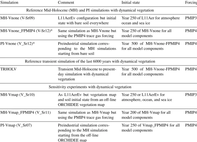
response is flatter than the shape of the seasonal insolation forcing, which leads to a poor projection over midlatitude and high-latitude ocean especially in the ocean-dominated SH (Fig. 7). Sea-ice cover has also little change north of 80◦N, which also damps the changes in seasonality (Fig. 8). These changes are, however, amplified by the increase in sea ice during summer in the Arctic resulting from cooler conditions with time and by the reduction in the winter sea-ice cover in the Labrador and the Greenland–Iceland–Nordic seas (Fig. 8a, b). For snow cover the conditions are contrasted depending on the regions (Fig. 8a, b, d), with an decrease in the maximum cover over Eurasia related to a long-term rise in minimum temperature (Fig. 8d)

3.3 Long-term vegetation trends

These long-term climate evolutions have a counterpart on the long-term evolution of vegetation (Fig. 9). At the global and hemispheric scale, the long-term vegetation trends corre-spond to reductions or increases in the area covered by veg-etation, reaching 2 % to 4 % of the total land area depending on vegetation type (Fig. 9). The global vegetation averages reflect the Northern Hemisphere changes where most of the vegetated continental masses are located. As expected from the different long-term trends in insolation, the long-term evolution of tree and grass cover is the opposite in the two hemispheres. Note, however, that bare soil slightly increases in both hemispheres.

Figure 8.(a) Total change in snow cover (kg m−2) and sea-ice fraction (%) integrated over the last 6000 years, and evolution from the Mid-Holocene of annual mean maximum summer and minimum winter values for (b) sea-ice averages over the Northern Hemisphere, (c) snow (solid lines) and 2 m air temperature (dotted lines) averaged for all regions north of 60◦N, and (d) snow and 2 m air temperature over Eurasia. In (b, c), and (d) black, dark blue and light blue stand, respectively, for the annual mean, maximum, and minimum annual monthly values for sea-ice or snow cover, and black, green, and red stand for annual mean, minimum, and maximum air temperature.

In the Northern Hemisphere the changes follow the changes in summer temperature, with the best match ob-tained for grass, which increases almost linearly until 2000 BP and then remains quite stable. In the Southern Hemisphere the phasing between vegetation change and tem-perature is not as good, again because this hemisphere is dominated by ocean conditions rather than land conditions. However, the tree expansion reaches a maximum between 2000 and 1000 BP, and then the tree cover slightly decreases, which corresponds to the slight cooling in SH summer tem-perature. The gross primary productivity (GPP; Fig. 9d) is driven in both hemispheres by the changes in tree cover. It accounts for a reduction of about 5 PgC yr−1. It is, however, possible that the GPP change is misestimated in this simu-lation because CO2 is prescribed in the atmosphere, which

implies that the carbon cycle is not fully interactive. Figure 10 compares the vegetation map obtained for the preindus-trial period in TRHOLV (150–100 BP) with MH vegetation. It shows that bare soil increases in semiarid regions in Africa and Asia as well as in southern Africa and Australia. The reduction in tree PFTs is maximal north of 60◦N, in south and southeast Asia, the Sahel, and most of North America. Tree PFTs are replaced by grass PFTs. In the Southern

Hemi-sphere, forest cover increases in southern Africa, southeast South America, and part of Australia.

In the last 100 years the effect of trace gases and in par-ticular the rapid increase in the atmospheric CO2

concen-tration leads to a rapid vegetation change characterized by tree regrowth, which is dominant in the NH (Figs. 9 and 10). This tree recovery counteracts the reduction from the Mid-Holocene in mid- and high NH latitudes (Fig. 10b, e, and h). This effect is consistent with the observed historical growth in gross primary production discussed by Campbell et al. (2017). The GPP increase in the last 100 years results from increased atmospheric CO2. It suggests that the CO2

ef-fect counteracts the tree decline induced by insolation. When reaching 0 BP (1950 CE), bare soil remains close to PI, grass is reduced by 3 %, and trees are increased by about 3 %.

3.4 Regional trends

Figure 11 highlights the long-term vegetation trends for three regions that, respectively, represent climate conditions north of 60◦N, over the Eurasian continent, and in the West African monsoon Sahel–Sahara region. These are regions for which there are large differences in MH–PI climate and veg-etation cover (Figs. 9 and 10). They have also been chosen

Figure 9. Long-term evolution of the simulated (a) bare soil, (b) grass, and (c) tree covers, expressed as the percentage (%) of global, NH, or SH continental areas, and (d) GPP (PgC yr−1) over the same regions. Annual mean values are smoothed by a 100-year running mean.

because they are widely discussed in the literature and are also considered as tipping points for future climate change (Lenton et al., 2008). They are well suited to provide an idea of different characteristics between regions.

North of 60◦N a substantial reduction in trees at the ex-pense of grass starts at 5000 BP (Fig. 11a, b). Vegetation almost reaches its preindustrial conditions around 2500 BP. The largest trends are found between 5000 and 2500 BP in this region, and this reflects the timing of the NH sum-mer cooling well. The change in total forest in Eurasia is small. A first change is followed by a second one around 3000 BP. Despite the 100-year smoothing applied to all the curves, they exhibit large decadal to multi-centennial vari-ability. Over West Africa (Fig. 11c), the largest trends start slightly later (4500–5000 BP) and are more gradual until 500 BP. The vegetation trends are also punctuated by several

centennial events that do not alter the long-term evolution as much as some of these events do in the other two boxes.

The variability found for vegetation is also found in tem-perature and precipitation at the hemispheric scale (Fig. 6). It is even higher at the regional scale in midlatitudes and high latitudes (Fig. 8). This variability is not present in the imposed forcing. It results from internal noise. Because of this it is difficult, for example, to say whether the NH winter temperature trend was rapid until 4000 BP and then ture remains stable or whether the event impacting tempera-ture and precipitation around 4800 to 4500 BP masks a more gradual increase until 3000 BP, as is the case for NH sum-mer where the magnitude of the temperature trend is larger than its variability (Fig. 6). Note that some of these internal fluctuations reach half of the total amplitude of the regional vegetation trends (Fig. 11) and that they are a dominant sig-nal over Eurasia, where the long-term mean change in the total tree cover is small (Figs. 10 and 11). Temperature and precipitation are well correlated at this centennial timescale (Fig. 6).

Despite the dry bias over the Sahel region in this version of the model, the timing of the vegetation changes over West Africa reported in Fig. 11 is consistent with the major fea-tures discussed for the end of the African humid period (Liu et al., 2007; Hély et al., 2014). In particular, the replacement of grass by bare soil starts earlier than the reduction in the tree cover located further south (Fig. 11). At the scale of the Sahel region, we do not have abrupt changes in vegetation but gradual ones. It is, however, abrupt at the grid cell level. These changes are associated with the long-term decline in precipitation, as well as the southward shift of the tropical rain belt associated with the African monsoon (Fig. 12). The location (latitude) of the rain belt is estimated here as the location of the maximum summer precipitation zonally av-eraged between 10◦W and 20◦E over West Africa. Most of the southward shift of the rain belt occurs between MH and 3500 BP and corresponds to a difference of about 1.8◦N of latitude over this period. Then the southward shift is smaller, with a total shift of 2.5◦N of latitude diagnosed in this sim-ulation. The comparison of Figs. 11 and 12 clearly shows that the rapid decrease in vegetation occurs after the rapid southward shift of the rain belt. An interesting point is that the amount of precipitation is also shifted in time compared to the location of the rain belt. It suggests that the vegeta-tion feedback on precipitavegeta-tion is still effective during the first period of precipitation decline and that it might have ampli-fied the reduction in precipitation when vegetation is reduced over the Sahel region.

As seen in Fig. 10, the NH decrease in forest cover is mainly driven by the changes that occur north of 60◦N (Figs. 8 and 10). These trends reflect more or less what is expected from observations (Bigelow et al., 2003; Jansen et al., 2007; Wanner et al., 2008). It results from the summer cooling that affects both the summer sea-ice cover in the Arc-tic, the summer snow cover over the adjacent continent, and

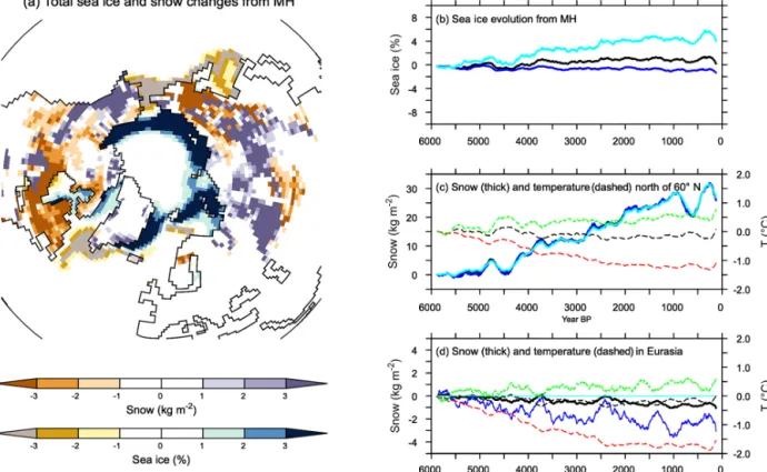
Figure 10.Vegetation map comparing (a, d, g) the Mid-Holocene (first 50 years) and the preindustrial (50 years around 1850 CE (150 to 100 BP)) periods of the transient simulation, (b, d, h) the differences between the historical period (last 50 years) and the preindustrial period of the transient simulation, and (c, f, i) the difference between preindustrial climate for the transient simulation and the PI-Vnone simulations. For simplicity we only consider bare soil (a–c), grass (d–f), and trees (g–i).

the amplification of the insolation forcing south of 70◦N by snow–vegetation albedo feedback. Further south over Eura-sia, Fig. 11 suggests that there are only marginal changes in Eurasia in terms of vegetation. Figure 13 shows that the total tree cover over this region does not reflect the mosaic veg-etation and forest composition well. Indeed, the long-term decrease in forest is dominated by the decrease in temperate and boreal deciduous trees. Boreal needleleaf evergreen trees do not change, whereas the temperate ones increase. This fig-ure also highlights that the long-term change in Eurasian tree composition throughout the Mid- to late Holocene is punc-tuated by centennial variability. The different trees also have different timing and variability. Boreal forests are more sen-sitive to variability during the first 3000 years of the simu-lation, whereas temperate broadleaf trees exhibit larger vari-ability in the second half. The large events have a climatic counterpart (Fig. 8), so that the composition of the vegetation is a result of a combined response to the long-term climatic change and to variability. These two effects can lead to differ-ent vegetation composition depending on stable or unstable vegetation states (Scheffer et al., 2012). Decadal vegetation changes have been discussed for recent climate in these

re-gions (Abis and Brovkin, 2017), which suggests that despite the fact that our dynamical vegetation model might under-estimate vegetation resilience, the rapid changes in vegeta-tion mosaic are a key signal over Eurasia. Future model–data comparisons should consider composition changes and vari-ability to properly discuss vegetation changes over this re-gion.

4 Vegetation, uncertainties, and multiple vegetation states

4.1 Simulated versus reconstructed vegetation

Section 3 shows how climate and vegetation respond to inso-lation and trace gases. The simulated changes are in broad agreement with what is expected from various sources of data. However, Sect. 2 mentions model adjustments and bi-ases. They all contribute to the difficulty of producing the right vegetation changes in the right place, at the right time, and for the right reasons. It is thus important to fully under-stand what we can expect in terms of realism from this sim-ulation. We investigate it for the Mid-Holocene and modern

Figure 11.Long-term evolution of bare soil, grass, and trees, ex-pressed as the percentage of land cover north of 60◦N, over Eura-sia, and over West Africa. The different values are plotted as differ-ences with the first 100-year averages. A 100-year running mean is applied to the curves before plotting.

Figure 12.Evolution of (a) the location of the West African mon-soon annual mean (black) and maximum (red) rain belt in degrees of latitude and (b) annual mean (black), minimum (green), and maxi-mum (red) monthly precipitation (mm d−1) averages over the Sahel region. The first 100 years have been removed and a 100-year run-ning mean applied before plotting.

climate, for which we can use the BIOME6000 vegetation reconstruction (Harrison, 2017).

The dynamical vegetation module simulates fractional cover of 13 PFTs. These PFTs cannot be directly compared with the reconstructed biome types based on pollen and plant macrofossil data from the BIOME 6000 dataset (Harrison,

2017). In order to facilitate the comparison, we converted the simulated PFTs into eight mega-biomes, using the biomiza-tion method algorithm proposed by Prentice et al. (2011). The algorithm uses a mixture of simulated climate and vege-tation characteristics (see Appendix and Fig. A2). Alternative thresholds as proposed in previous studies (Joos et al., 2004; Prentice et al., 2011) were tested to account for the uncer-tainties in the biomization method (see Fig. A2). At a first glance MH-Vnone reproduces the large-scale pattern found in the BIOME6000 reconstruction (Fig. 14a). The compari-son, however, indicates that the boreal forest tree line is lo-cated too far south. It results from a combination of a cold bias in temperature in these regions and a systematic un-derestimation of forest biomass in Siberia with ORCHIDEE when forced by observed present-day climate (Guimberteau et al., 2018). Such underestimation of tree biomass could lead to too low a tree height in ORCHIDEE and thus to the replacement of boreal forest by dry woodland accord-ing to the biomization algorithm (Fig. A2a). Also, vegeta-tion is underestimated in West Africa, consistent with a dry bias (not shown). The underestimation of the African mon-soon precipitation is present in several simulations with the IPSL model (Braconnot and Kageyama, 2015) and is slightly enhanced in summer when the dynamical vegetation is ac-tive. With interactive vegetation, however, equatorial Africa is more humid (Fig. 15a). Figure 14c provides an idea of the major mismatches between simulated vegetation and the BIOME6000 reconstructions. In particular, the simulation produces too much desert where we should find grass and shrubs. It also produces too much tundra instead of boreal forest and too much savannah and dry woodland in several places that should be covered by temperate trees, boreal trees, or tundra, confirming the visual map comparison (Fig. 14c). Similar results are found when considering the preindustrial climate in TRHOLV compared to the BIOME6000 preindus-trial biome reconstruction (Fig. A2d). These are systematic biases. These systematic biases are confirmed when compar-ing the simulated PFTs for PI with those of the 1860 CE map estimated from observations and used in simulations with prescribed vegetation (see Table A1 for regions without land use).

It is not possible to estimate the vegetation feedback on the long-term climate evolution from the transient simula-tion. It is, however, possible to infer how the dynamical veg-etation affects the mean climatology for the MH, a period for which simulations with prescribed and dynamic vege-tation are available. Metrics discussed in Sect. 2.4 (Fig. 3) show that the introduction of the dynamical vegetation in the model reduces the amount of precipitation and that the climate is dryer. The simulations with dynamical vegetation only consider natural vegetation, whereas the 1860 CE map we prescribe when vegetation is fixed includes land use. In regions affected by land use, all MH simulations produce less bare soil (3 %), more tropical trees (5 %), similar temperate tree cover, increased boreal tree cover (10 %), and a

differ-Figure 13.Evolution of the different tree PFTs in Eurasia, expressed as the percentage change compared to their 6000 BP initial state. Each colored line stands for a different PFT. Values have been smoothed by a 100-year running mean.

Figure 14.(a) Simulated mega-biome distribution by MH-Vnone, converted from the modeled PFT properties using the default algorithm described in Fig. A1. Panels (b) and (c): reconstructions in BIOME 6000 DB version 1 for the MH and PI periods (Harrison, 2017). (d) Number of pixels where reconstruction is available and the model matches (or does not match) the data. Note that multiple reconstruction sites may be located in the same model grid cell, in which case we did not group them so that each site was counted once. Numbers in parentheses on the x axis in (d) represent the number of sites for each biome type. Panel (e) same as (c) but for the number of matches between (e) the BIOME6000 MH (6 k) and PI (0 k) reconstructions at pollen sites and (f) the simulated mega-biomes for MH and PI at each model grid cell.

ent distribution between C3 versus C4 grass (see Table A1). In Eurasia where croplands are replaced by forest, the lower forest albedo induces warmer surface conditions (Fig. 15b). Also, when snow combines with forest instead of grasses, the snow–vegetation albedo is lower, leading to the positive snow–forest feedback widely discussed for the last glacial inception (de Noblet et al., 1996; Kutzbach et al., 1996). Fig-ure 15a also highlights that precipitation is increased over the African tropical forest and reduced over South America. In most regions the impact of vegetation is much smaller than the impact of the changes in the land surface hydrology and forcing strategy discussed in Sect. 2.3 (Fig. 2).

The differences between the MH simulated vegetation map and the 1860 CE map reflect both systematic model bi-ases and vegetation changes related to the MH climate dif-ferences with PI. We can infer from Figs. 15 and 16 that vegetation has a positive warming feedback in the high lat-itudes during MH. Part of the differences between the MH and the PI conditions in Fig. 15c, d is dominated by the impact of vegetation. Similar patterns as those obtained for the impact of vegetation are found over Eurasia for tempera-ture, or southeast Asia and North America for precipitation. For the grid points where BIOM6000 data are available for both MH and PI (0 k – 1860 CE), the major simulated biome changes occur for savannah and wood and grass and shrubs (Fig. 14e). Differences are also found for trees and tundra, but to a lesser extent. The comparison with similar estimates from BIOME6000 reconstructions indicates that grass and shrubs exhibit major changes and that trees show larger dif-ferences compared to the simulation. The model shift be-tween savannah and wood and grass and shrubs is consistent with the noted bias for savannah and the fact that the tree cover is underestimated in NH latitudes (Fig. 14).

Note that the vegetation differences found between the his-torical period and the PI period in TRHOLV are not negligi-ble. We can estimate from Fig. 15a, b that neglecting land use leads to an underestimation of about 1◦C in Eurasia between the MH and PI in this TRHOLV simulation. Depending on whether PI or the historical period is used as a reference, the magnitude of the MH changes in vegetation and climate are different. Also, land use has regional impacts and should be considered in PI or in the historical period. This stresses that a quantitative model–data comparison must be treated with caution, knowing that both the reference period (PI or histori-cal) and the complexity of the land surface model (prescribed vegetation, natural dynamical vegetation, land use . . . ) can easily lead to 1◦_{C difference in some regions.}

4.2 Multiple vegetation states for the preindustrial climate

Another source of uncertainty concerns the stability of the simulated vegetation maps. Several studies suggest that the initial state only has a minor impact on the final climate be-cause there is almost no change in the thermohaline

circula-tion over this period and models do not exhibit major climate bifurcations (e.g., Bathiany et al., 2012). This is the main ar-gument used by Singarayer and Valdes (2010) to justify that their suite of snapshot experiments may provide a reasonable transient climate vision when put together. Is this the case in the TRHOLV simulation when vegetation is fully interac-tive? This transient simulation does not exhibit much change in the indices of thermohaline circulation, which remains close to 16–18 Sv (sverdrup) (1 Sv = 106m3s−1) through-out the period. The global metrics (Fig. 3) show that at the global scale the results of the TRHOLV simulations for PI (1860 CE) are similar to those of PI-Vnone. It is also the case for seasonal and extratropical or tropical values (Fig. A1). We can therefore conclude that there is no difference in mean surface climate characteristics between the snapshot PI-Vnone experiments and the PI period simulated in the transient TRHOLV simulation.

Is the vegetation then also similar to the one simulated in PI-VNone? The PI vegetation simulated in TRHOLV shows little differences to the one found for PI-Vnone (Fig. 10c, f, and i). The relative percentages of land cov-ered by the different vegetation classes correspond to 15 % for bare soil, 41 % for grass, and 43 % for trees, respectively. These values are similar to the one found for PI-VNone (15 %, 40 %, and 44 %, respectively) within 1 % error bar. This does not necessarily hold at the regional scale where re-gional differences are also found between PI-TRHOLV and PI-Vnone. Indeed, Fig. 10 indicates differences in tree and grass cover in Eurasia around 60◦N and different geographi-cal coverage between bare soil, grass, and trees over southern Africa and Australia. These differences are very small com-pared to the differences between MH and PI in TRHOLV, but are as large as the difference between historical (i.e., the last 50 years of the simulation) and PI in a few places in Eurasia. As seen in previous section, these are regions where variabil-ity is large and vegetation instable.

We also tested whether the PI vegetation and climate would also be similar when starting from MH-Vmap instead of MH-Vnone (dark pink and orange lines in Fig. 4d–f). This is also a way to have a better idea of the range of response one would expect from ensemble simulations, knowing that we only ran one full transient simulation. For the PI-Vmap sim-ulation, the orbital parameters and trace gases were first pre-scribed to preindustrial conditions for 15 years while main-taining the vegetation PFTs in each grid cell to those obtained in MH-Vmap (Table 2, Fig. 4). Then, the dynamical vege-tation was switched on. It induces a rapid transition of the major PFTs that takes about 10 years before a new global equilibrium is reached (Fig. 4d–f). For PI-VNone presented in Sect. 2.4 the same procedure was applied, but the dynam-ical vegetation was switched on after 5 years (Table 2 and Fig. 4), and the new equilibrium state is reached without any relaxation or rapid transition.

PI-Vnone and PI-Vmap converge to different global veg-etation states (Fig. 4). Compared to the values listed above

Figure 15.Impact of the dynamical vegetation and initialization of vegetation on the simulated climate. Differences for annual mean (a, c, e) precipitation (mm d−1) and (b, d, f) 2 m air temperature (◦C) between (a) the MH in the TRHOLV simulation and (b) the MH simulation without dynamical vegetation (MH FPMIP4), (c) the Mid-Holocene and (d) the preindustrial simulations in the TRHOLV simulation, and (e) and (f) the two preindustrial simulations initialized from bare soil (PI-Vnone) or a vegetation map for vegetation (PI-Vmap). See Table 2 and text for details on the simulations.

for PI-Vnone and PI-TRHOLV the respective covers of bare soil, grass, and trees for PI-Vmap are 20 %, 37 %, and 43 %. In particular, PI-Vmap produces a larger bare soil cover than PI-Vnone (Fig. 4d). It is even larger than the total bare soil cover found in the 1860 CE map used in PI simulations when vegetation is prescribed (Fig. 4). Interestingly part of these differences between Vmap and Vnone is found in the South-ern Hemisphere and the northSouth-ern edge of the African and Indian monsoon regions. Since there is almost no difference in MH vegetation between Vmap and Vnone, these differ-ences in PI vegetation drive the vegetation differdiffer-ences be-tween MH and PI (Fig. 16). The MH simulated changes seem larger with Vmap. A previous assessment of model results against vegetation and paleoclimate reconstructions (e.g., Harrison et al., 1998, 2014) suggests that MH–PI vege-tation for Vmap would be in better agreement with recon-structed changes from observations in terms of forest ex-pansion in the Northern Hemisphere or grasses in the Sahel (Fig. 16). However, the modern vegetation map for this PI-Vmap simulation has even less forest than PI-Vnone north of 55◦N (Fig. 4e, f, and i), for which forest is already under-estimated (Fig. A2). These differences in PI vegetation only have a small counterpart in climate. These biases correspond

to cooler condition in the midlatitudes and high northern lat-itude (Fig. 15). In the annual mean, there is almost no im-pact on precipitation (Fig. 15). In terms of climate these two simulations are very similar and closer to each other than to other simulations, whatever the season or the latitudinal band (Fig. A1). The small differences in climate listed above are thus too small to be captured by global metrics. It suggests that there is no direct relationship between the different veg-etation maps and model performances. The different vege-tation maps are obtained with a similar climate, which indi-cates that in this model multiple global and vegetation states are possible under preindustrial climate or that tiny climate differences can lead to different vegetation.

5 Conclusion

This long transient simulation over the last 6000 years with the IPSL climate model is one of the first simulations over this period with a general circulation model including a full interactive carbon cycle and dynamical vegetation. Several adjustments were made to set up the model version and the transient simulations. Most of them have a larger impact on the model climatology than the dynamical vegetation feed-back and remind us that fast feedfeed-backs occur in coupled

sys-Figure 16.Difference between Vegetation maps obtained with the two different initial states for (a, c, e) Mid-Holocene simulations and (b, d, f) preindustrial simulations. Vmap stands for MH and PI simulations where the Mid-Holocene vegetation has been initialized from a vegetation map and Vnone for MH and PI simulations where the Mid-Holocene has been initialized from bare soil. For simplicity we only consider fractions of (a, b) bare soil, (c, d) grass, and (e, f) trees.

tems so that any evaluation of surface flux should consider both the flux itself and the climate or atmospheric variables used to compute it (Torres et al., 2018). We show that, despite some model biases that are amplified by the additional degree of freedom resulting from the coupling between vegetation and climate, the model reproduces reasonably well the large-scale features in climate and vegetation changes expected from reconstructions over this period. The transient simula-tion exhibits little change in annual mean climate through-out the last 6000 years (not shown). The seasonal cycle is the main driver of the climate and vegetation changes, ex-cept in the last part of the simulation when the rapid green-house gas concentration increase leads to rapid global warm-ing. There has been lots of discussion regarding the sign of the trends in the northern midlatitudes following the results of the first coupled ocean–atmosphere simulation with the CCSM3 model across deglaciation (Liu et al., 2014). Our

re-sults seem in broad agreement with the 6000 to 0 BP part of the revised estimates by Marsicek et al. (2018).

The analysis of vegetation differences between PI-Vmap and PI-VNone once more raises the possibility of multiple vegetation equilibrium under preindustrial or modern condi-tions, as has been widely discussed previously (e.g., Brovkin et al., 2002; Claussen, 2009). Here we have both global and regional differences. Our results are, however, puzzling because we only find limited differences between the PI-Vnone snapshot simulation and the PI climate and vegeta-tion produced at the end of TRHOLV. These simulavegeta-tions start from the same initial state and in one case PI condi-tions are switched on in the forcing, whereas in the other case the 6000-year long-term forcing in insolation and trace gases is applied to the model. An ensemble of simulations would be needed to fully assess vegetation stability. In the North-ern Hemisphere and over forest areas, MH-Vmap produced slightly fewer trees that MH-Vnone. It might have been

am-should not be the case because it would not explain why veg-etation is sensitive to the initial state in PI and not in MH. It is also possible that the climate instability induced by the change from one year to the other in insolation and trace gases leads to rapid amplification of climate at high latitudes, which is more effective under the cooling high-latitude con-dition found in PI. The strongest conclusion from these sim-ulations is that the vegetation–climate system is more sensi-tive under preindustrial conditions (at least in the Northern Hemisphere).

Our analyses show that the MH–PI changes in climate and vegetation are similar between snapshot experiments and in the long transient simulation. What, then, is the added value of the transient simulation? The good point is that model evaluation can be done on snapshot experiments, which fully validate the view that the Mid-Holocene is a good period for model benchmarking in the Paleoclimate Modeling Inter-comparison Project (Kageyama et al., 2018). However, the MH–PI climate conditions mask the long-term history and the relative timing and the rate of the changes. The major changes occur between 5000 and 2000 BP and the exact tim-ing depends on regions. In our simulation the forest reduc-tion in the Northern Hemisphere starts earlier than the vege-tation changes in Africa. It also ends earlier. The last period reflects the increase in trace gases with a rapid regrowth of trees in the last 100 years when CO2 and temperature

in-crease at a rate not seen over the last 6000 to 2000 years. Some of these results already appear in previous simulations with intermediate-complexity models (Crucifix et al., 2002; Renssen et al., 2012). Using the more sophisticated model with a representation of different types of trees brings new results. Even though the total forest cover does not vary much throughout the Holocene in TRHOLV, the composition of the forest varies more substantially, with different relative timing between the different PFTs.

We mainly consider here surface variables that have a rapid adjustment with the external forcing. Also, we only consider long-term trends in this study, but the results highlight that centennial variability plays an important role in shaping the response of climate and vegetation to the Holocene external forcing at a regional scale. In-depth anal-yses of ice-covered regions and of the ocean response would

in the introduction: (1) insolation is the main driver of the climate and vegetation in the NH and in the SH for summer and the response to the insolation forcing north of 80◦N, and in the SH it is muted by ocean or sea-ice and snow feed-back; (2) the impact of the trace gases is effective in the last 100 years of the simulation and counteracts the effect of the Holocene insolation on both climate and vegetation in the NH and enhances it in the SH; (3) the timing of the vegetation changes depends on region with tree regression starting first at high NH latitudes; (4) centennial variability is large and needs to be accounted for to understand regional changes, in particular over Eurasia. This has implications for model– data comparison. High-resolution records from tree rings, speleothems, or varved sediments are unique records to as-sess climate variability, but they are sparse and most of them span noncontinuous periods of time. The model framework, even though it is an imperfect representation of reality, offers a consistent framework to discuss the consistency between records. To go further in this direction, a specific methodol-ogy needs to be designed to assess the climate–vegetation dynamics over a long timescale without putting too much weight on inherent model biases. Another difficulty in prop-erly assessing these model results against paleoclimate re-constructions is related to the fact that we only represent natural vegetation and neglect land use and aerosols other than dust and sea salt. Therefore the PI and historical climate cannot be realistically reproduced, even though most of the characteristics we report are compatible with what has been observed. In addition, the magnitude of the simulated differ-ences between MH and modern conditions depends on the reference period. This opens new challenges for model–data comparisons to properly analyze the pace of changes and cli-mate variability. It suggests that more needs to be done to derive criteria allowing us to assess the processes leading to the observed changes rather than to assess the changes them-selves.

Data availability. The transient simulation was run as part of the JPI-Belmont project PACMEDY. The data are available upon re-quest to pascale.braconnot@lsce.ipsl.fr.