HAL Id: hal-00296252
https://hal.archives-ouvertes.fr/hal-00296252
Submitted on 14 Jun 2007
HAL is a multi-disciplinary open access
archive for the deposit and dissemination of
sci-entific research documents, whether they are
pub-lished or not. The documents may come from
teaching and research institutions in France or
abroad, or from public or private research centers.
L’archive ouverte pluridisciplinaire HAL, est
destinée au dépôt et à la diffusion de documents
scientifiques de niveau recherche, publiés ou non,
émanant des établissements d’enseignement et de
recherche français ou étrangers, des laboratoires
publics ou privés.
smoke event in the European Arctic and its radiative
impact
R. Treffeisen, P. Tunved, J. Ström, A. Herber, J. Bareiss, A. Helbig, R. S.
Stone, W. Hoyningen-Huene, R. Krejci, A. Stohl, et al.
To cite this version:
R. Treffeisen, P. Tunved, J. Ström, A. Herber, J. Bareiss, et al.. Arctic smoke ? aerosol characteristics
during a record smoke event in the European Arctic and its radiative impact. Atmospheric Chemistry
and Physics, European Geosciences Union, 2007, 7 (11), pp.3035-3053. �hal-00296252�
www.atmos-chem-phys.net/7/3035/2007/ © Author(s) 2007. This work is licensed under a Creative Commons License.
Chemistry
and Physics
Arctic smoke – aerosol characteristics during a record smoke event
in the European Arctic and its radiative impact
R. Treffeisen1, P. Tunved2, J. Str¨om2, A. Herber3, J. Bareiss4, A. Helbig4, R. S. Stone5, W. Hoyningen-Huene6, R. Krejci7, A. Stohl8, and R. Neuber1
1Alfred Wegener Institute for Polar and Marine Research, Telegrafenberg A45, 14473 Potsdam, Germany 2ITM – Department of Applied Environmental Science, Stockholm University, S 106 91 Stockholm, Sweden 3Alfred Wegener Institute for Polar and Marine Research, Am Handelshafen 12, 27570 Bremerhaven, Germany 4University of Trier, Department of Climatology, 54286 Trier, Germany
5Cooperative Institute for Research in Environmental Sciences, University of Colorado, Boulder 80309, USA 6University of Bremen, Institute of Environmental Physics, Otto-Hahn-Allee 1, 28334 Bremen, Germany 7Department of Meteorology (MISU), Stockholm University, S 106 91 Stockholm, Sweden
8Norwegian Institute for Air Research, Instituttveien 18, 2027 Kjeller, Norway
Received: 28 November 2006 – Published in Atmos. Chem. Phys. Discuss.: 16 February 2007 Revised: 21 May 2007 – Accepted: 27 May 2007 – Published: 14 June 2007
Abstract. In early May 2006 a record high air pollution event was observed at Ny- ˚Alesund, Spitsbergen. An atypical weather pattern established a pathway for the rapid transport of biomass burning aerosols from agricultural fires in East-ern Europe to the Arctic. Atmospheric stability was such that the smoke was constrained to low levels, within 2 km of the surface during the transport. A description of this smoke event in terms of transport and main aerosol characteristics can be found in Stohl et al. (2007). This study puts empha-sis on the radiative effect of the smoke. The aerosol num-ber size distribution was characterised by lognormal param-eters as having an accumulation mode centered around 165– 185 nm and almost 1.6 for geometric standard deviation of the mode. Nucleation and small Aitken mode particles were almost completely suppressed within the smoke plume mea-sured at Ny- ˚Alesund. Chemical and microphysical aerosol information obtained at Mt. Zeppelin (474 m a.s.l) was used to derive input parameters for a one-dimensional radiation transfer model to explore the radiative effects of the smoke. The daily mean heating rate calculated on 2 May 2006 for the average size distribution and measured chemical composi-tion reached 0.55 K day−1at 0.5 km altitude for the assumed external mixture of the aerosols but showing much higher heating rates for an internal mixture (1.7 K day−1). In
com-parison a case study for March 2000 showed that the local climatic effects due to Arctic haze, using a regional climate model, HIRHAM, amounts to a maximum of 0.3 K day−1of heating at 2 km altitude (Treffeisen et al., 2005).
Correspondence to: R. Treffeisen ([email protected])
1 Introduction
The Arctic atmosphere is extremely clean. Since the 1950s, however, a haze has been observed there each spring (Green-away, 1950; Mitchell, 1957). This phenomenon, referred to as Arctic haze is in large part due to anthropogenic aerosols being transported into the Arctic throughout the winter and early spring. A good overview of the history and early stud-ies of Arctic haze can be found in Barrie (1986) and Shaw (1995). Since its discovery, chemical properties of this haze have been measured in several locations ranging from Alaska to Greenland, the European Arctic and the Central Arctic Ocean (e.g. Heintzenberg, 1981; Barrie et al., 1990; Hopfer et al., 1994; Leck et al., 2001; Ricard et al., 2002, and ref-erences therein). Numerous investigations have been under-taken to understand sources, occurrences and transport path-ways (e.g. Norman et al., 1999; MacDonald et al., 2000; Stohl 2006, and references therein).
The direct radiative effect of Arctic haze has been inves-tigated using one-dimensional radiative transfer models (e.g. Emery et al., 1992; Shaw et al., 1993). The results of these studies show that solar radiation is absorbed within the at-mosphere in the amount of 2 to 20 W m−2and cause heat-ing in the range of 0.1 and 1.8 K day−1. At the surface, however, the net solar flux is reduced by 0.2 to 6 W m−2, which results in surface cooling. In the unperturbed atmo-sphere, the clear-sky radiative cooling is about 1 K/day. The calculated heating/cooling magnitudes were strongly depen-dent on the assumed optical properties of the aerosol deter-mined by the concentration, chemical composition, number size number distribution and atmospheric humidity. Forcing
of the atmosphere and surface is also a function of solar zenith angle and surface albedo. The evaluation of the di-rect climatic and indidi-rect effects of Arctic aerosols requires the use of complex three-dimensional climate models. An estimation with a global circulation model revealed strong, regionally varying effects at the surface; in the Arctic char-acterised as a warming of 1 to 2 K (Blanchet, 1989). Even within the Arctic, aerosol distributions are highly variable, in both space and time. The coarse spatial resolution of global climate models cannot account for this variation (Barrie et al., 2001). Therefore, the use of high resolution regional cli-mate models covering the Arctic is recommended. Regional climate models have a typical horizontal resolution of 15– 50 km and provide the same complexity concerning physical processes as global models. For instance, a case study for March 2000 showed that the regional climatic effects due to Arctic haze, on the basis of airborne measurements using a regional climate model, HIRHAM, amounts to between 0.05 and 0.3 K day−1of heating in the altitude up to 2 km (Tref-feisen et al., 2005).
In this paper, we evaluate another kind of Arctic air pollu-tion, namely smoke from biomass burning in Eastern Europe during late April and beginning of May 2006. Many studies showed that emissions from agricultural and forest fires not only constitute local pollutants, but are also transported away from sources and have the potential to affect global atmo-spheric chemistry (e.g., Fishman, 1991; Levine, 1996; Har-vey et al., 1999; Rinsland et al., 1999), and also in the Arctic (Stohl et al., 2006a). Research has also shown that aerosols from such fires directly and indirectly affect radiative forcing (e.g., Konzelmann et al., 1996; Wild, 1999; French, 2002). In addition, aerosol-cloud interactions (indirect effect) are cur-rently considered to be one of the most important and uncer-tain drivers of climate change. Recent research has shown that aerosols from heavy smoke modify cloud droplet size, delaying the onset of precipitation (e.g, Robock, 1991; Ra-manathan et al., 2001; Andreae et al., 2004).
Specific data for peatland burning in Siberia are limited and therefore difficult to assess (e.g., Davidenko and Eritsov, 2003; Goldammer, 2003). Northern peatlands hold one third of the soil organic matter on Earth and the amount of carbon stored in peatlands per square meter is typically larger than that held in forested zones. Agricultural fires were found to account for 8–11% of the annual global fire activity dur-ing 2001 and 2003, but the contribution of agricultural burn-ing biomass was significantly higher on a regional basis (Ko-rontzi et al., 2006). The Russian Federation was the largest contributor to agricultural burning globally producing 31– 36% of all agricultural fires (Korontzi et al., 2006).
Between 27 April and the first days of May 2006 the most severe air pollution ever registered at Ny- ˚Alesund, Svalbard was recorded. This event resulted from the transport of smoke from fires in Belarus, the northern parts of Ukraine and Western Russia (Stohl et al., 2007). Due to dry weather, fires burned extensively over an area of about 20 000 square
kilometres. We describe the synoptic-scale meteorological characteristics and flow patterns in Eastern and Northern Eu-rope that promoted the rapid transport of this smoke into the Arctic region. Satellite measurements of aerosol optical depth (AOD) are used to demonstrate the horizontal extent of the plume. Finally, in situ measurements of the aerosol are examined to characterize the smoke that arrived at
Ny-˚
Alesund. Using derived optical properties we then estimate atmospheric heating rates using a one-dimensional radiative transfer model.
2 Model description for radiative transfer calculations
2.1 Mie scattering code
Aerosol optical properties are estimated using the Mie code, MIEV0, by Wiscombe (1979). MIEV0 relies on input of Mie size parameter and complex refractive index to yield the scattering and extinction efficiency as well as the asymmetry parameter of individual particles. On the basis of the mea-sured aerosol number size distribution the optical properties of internal or external mixtures are computed with a given chemical composition. All particles in the entire size spec-trum are assumed to have the same chemical composition for internally mixed aerosols. For externally mixed particles each size of particles may have different composition, but the fraction of particles with a given composition is the same for all sizes. The reality is somewhere in-between these two ex-tremes. The particles are allowed to undergo hygroscopic growth assuming standardized hygroscopic growth factors for different compounds as presented in the Global Aerosol Data Set (GADS, K¨opke et al., 1997). In case of internal mixture, the growth factors of the mixture of different com-pounds are assumed additive, using the Zdanovskii-Stokes-Robinson (ZSR) assumption (Stokes and Zdanovskii-Stokes-Robinson, 1966).
The wavelength dependent refractive index of soot is taken from a parameterisation by Chang and Charalampopoulos (1990). The refractive index of sulphate, insoluble organ-ics, soluble organics and sea-salt are taken from the OPAC database (Hess et al., 1998). The Maxwell-Garnett approx-imation was used to calculate the refractive index of differ-ent mixtures of the compounds in the cases when internally mixed aerosol is assumed. We make the approximation that mass mixing ratios of the aerosol are identical to volume mixing ratios, i.e. assuming that all compounds have the same density. In fact, we do not know these densities. The scattering, extinction and absorption coefficients are then es-timated as: bext= r maxZ r min π r2Qext(m, α)Nrdr (1) babs= r maxZ r min π r2Qabs(m, α)Nrdr (2)
bsca=
r maxZ
r min
π r2Qsca(m, α)Nrdr (3)
with r=radius of the particle, Qext=extinction efficiency; Qsca=scattering coefficient; Qabs=absorption coefficients, m=refractive index, the size parameter of the particle and Nr=number of particles of radius r.
2.2 Radiative transfer code
The code used for the radiative transfer calculations is the Santa Barbara DISORT (discrete ordinate) Atmospheric Ra-diative Transfer (SBDART, Ricchiazzi et al., 1998). SB-DART includes all important processes affecting ultraviolet, visible and infrared radiation. The code includes options for discrete ordinate radiative transfer computations, low resolu-tion atmospheric transmission computaresolu-tions, and Mie codes for scattering by ice and water clouds. For this study, SB-DART is used to calculate the solar irradiance in the 0.25– 4 µm band for clear sky conditions only. This band captures the most important part of the solar spectrum that interacts with particles and allows for direct comparisons of heating rate calculations previously performed in the Arctic envi-ronment (Treffeisen et al., 2005). The atmospheric profile of ozone, pressure, relative humidity and temperature is es-timated as a combination of available routine soundings at Ny- ˚Alesund up to approximately 30 km and standard atmo-spheric profiles for sub-Arctic summer standard atmosphere provided by the SBDART. The vertical model resolution is set to 0.5 km in the lowermost 10 km, and above this level a vertical increment of 4 km up to 100 km is used.
The radiative transfer model requires specification of the AOD, single scattering albedo and Legendre moments of the phase function at each atmospheric layer. These parameters are derived from the Mie-scattering code. The Legendre mo-ments are defined according to the Henyey Greenstein ap-proximation of the phase functions (i.e. powers of the asym-metry parameter). The resolution of the wavelength is spec-ified with a step size of 0.05 times the previous wavelength. This causes a high resolution in the lower wavelength band, and a coarser resolution at higher wavelengths. The sur-face albedo is taken from ground-based measurements at
Ny-˚
Alesund and we have to assume a spectrally uniform surface albedo as the measurements are not available for different wavelengths.
3 Meteorological condition during the smoke episode
The first incursion of high concentration aerosols was ob-served at Svalbard on 27 April 2006, with peak concen-trations being measured on 2 to 3 May. These incursions resulted from rapid, meridional transport of polluted air (smoke) from source regions approximately 3900 km away in western Russia. Along the path no precipitation occurred
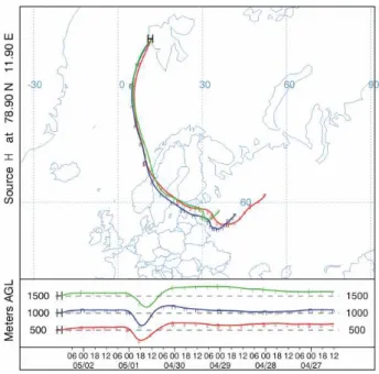
Fig. 1. Five days back trajectories at 500 m, 1000 m and 1500 m a.g.l. for the air mass arriving in Ny- ˚Alesund on 2 May 2006 (12:00 UTC) as computed by the HYSPLIT model. Data source: NOAA-ARL.
and therefore we conclude that there was no wet deposition. The following section describes specific synoptic conditions that favoured this unusual flow pattern. We also discuss the stability and vertical extent of the smoke plume that influ-ences calculations of heating rates presented in Sect. 5. 3.1 Trajectory analysis during the smoke episode
Back trajectories during the smoke episode have been com-puted using the NOAA HYbrid Single-Particle Lagrangian Integrated Trajectory (HYSPLIT) model provided by the Air Resources Laboratory (ARL) (Draxler and Rolph, 2003). In the particle model, a fixed number of initial particles are ad-vected about the model domain by the mean wind field and a turbulent component. Back trajectories were generated to visualize the atmospheric transport during burning events in western Russia (Fig. 1). The trajectories have been used to evaluate general flow patterns of air masses transported to Svalbard. The smoke released from fires in western Rus-sia on 26 April 2006 (12:00 UTC) arrived at Ny- ˚Alesund on 2 May 2006 (12:00 UTC), having an estimated mean trans-port velocity of about 650 km day−1. The fires actually began burning in that area around the middle of April but as shown by Stohl et al. (2007) the smoke arrived in Ny- ˚Alesund was only 3 to 4 days old. Similar weather patterns persisted dur-ing second half of April
On April 2006 and during the first days of May 2006 smoke arrived at Ny- ˚Alesund at the 1000 m level with an average speed of only 14 km h−1. The highest velocities
Fig. 2. Mean sea level pressure (hPa) (left) and absolute topography height contours at 850 hPa (right) over Europe during the period 26
April to 2 May 2006. Data source: NOAA-CIRES CDC.
Fig. 3. Daily means of sea level pressure (hPa) at the starting date of the parcel transport (26 April 2006) (left) and end date (2 May 2006)
(right) over Europe during the drift period. Data source: NOAA-CIRES CDC.
occurred in the last section of transport, reaching a maxi-mum of 48 km h−1over the Norwegian Sea. Hence, the pos-sibility for lateral diffusion and spreading of smoke was re-duced. Observed meteorological data from synoptic and ra-diosonde stations along the trajectories agree well with the atmospheric transport pattern obtained from the HYSPLIT model. In addition, detailed calculations of transport for the period from FLEXPART, a particle dispersion model (Stohl et al., 2007, http://zardoz.nilu.no/∼andreas/flextra+flexpart.
html) corroborate this analysis. 3.2 General circulation pattern
Over the period from the end of April to beginning of May 2006 the general atmospheric circulation in the northern hemisphere was characterised as having a low pressure sys-tem positioned north of Iceland with central pressure of about 1000 hPa coupled with a strong, quasi-stationary anticyclone centered over Eastern and North-eastern Europe. The
anti-cyclonic system extended from the surface level up to the middle troposphere with a central pressure of about 1035 hPa (Fig. 2, left). The mean sea level pressure over Eastern Eu-rope was calculated from NCEP/NCAR reanalysis data to be about 20 hPa higher than the long-term average for the pe-riod 1971 to 2000 in this region during the pepe-riod of interest. The corresponding geopotential height contours at 850 hPa are shown in the figure to the right. The pronounced high pressure system effectively blocked westerly winds and di-rected the flow northward.
During the observation period the anticyclone over Rus-sia moved gradually to Eastern Europe weakened by about 10 hPa (Fig. 3), while the low over the Atlantic (at 20◦W and 57◦N) deepened to about 980 hPa. This dipole pattern produced a strong, meridional circulation due to the extraor-dinary horizontal pressure gradient, a condition atypical for this time of the year.
Kiev (WMO 33345) 25/4/2006 12 UTC Kiev (WMO 33345) 26/4/2006 12 UTC 0 1000 2000 3000 4000 5000 6000 -60 -50 -40 -30 -20 -10 0 10 20 30 40 Black: Air Temp. [°C], Blue: Dew Point [°C],
Red: Pot. Temp. [°C]
H e ig h t [m ] 0 10 20 30 40 50 60 70 80 90 100
Green: Relative Humidity [%]
-60 -50 -40 -30 -20 -10 0 10 20 30 40 Black: Air Temp. [°C], Blue: Dew Point [°C],
0 1000 2000 3000 4000 5000 6000
Red: Pot. Temp. [°C]
H e ig h t [m ] 0 10 20 30 40 50 60 70 80 90 10
Green: Relative Humidity [%]
0
Figure 4. Vertical profiles of temperature and humidity at the radiosonde station Kiev (WMO
Fig. 4. Vertical profiles of temperature and humidity at the radiosonde station Kiev (WMO: 33345), Ukraine, on 25 April 2006 (left) and on
26 April 2006 (right), 12:00 UTC. Data source: NCDC, NOAA-FSL.
3.3 Atmospheric conditions during transport from western Russia to Svalbard
3.3.1 Source area/Western Russia
In spring, anticyclonic weather conditions are common for Eastern Europe which is characterised as having a transcon-tinental climate (Oliver, 2005). During the period from the middle of April to the first days of May 2006 anticyclonic cir-culation was particularly pronounced in this region (Fig. 3). The high pressure that persisted caused extremely warm con-ditions in which upper soil layers as well as vegetation be-came dry and prone to fire danger. Widespread fires ensured and burned for many days. Stable conditions in the lower tro-posphere constrained the dispersion of smoke plumes verti-cally and horizontally. The atmosphere was thermally stable or neutrally stratified to an altitude of 2.5 km as indicated by the 12:00 UTC radiosonde observations made over Kiev on 25 and 26 May 2006 (Fig. 4). Relative humidity increased continuously up to a height of about 2.5 km. Above, the air was very stable and RH dropped from roughly 60% to 15% within a 1000 m layer. The height of the convective bound-ary layer was about 2–2.2 km and the convective uplift was favoured by the heating of the smoke (Fig. 4). This warm, dry and very stable air mass was in place through the end of April which resulted in horizontal dispersion of the smoke over a wide area of western Russia. In contrast to forest fires with much higher heat flow densities, such as boreal forest fires, the fires in western Russia did not develop any “py-roCb” (pyrocumulonimbus) clouds that can reach very high altitudes. Furthermore, fires in western Russia consist of
nu-merous small fires distributed over a broad area (Stohl et al., 2007).
3.3.2 Meteorological conditions en route
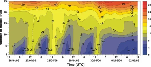
During the first days, the smoke clouds from the agricultural fires were transported with north-easterly winds to Eastern Europe to become south-easterly as they were swept by an-ticyclonic winds over Eastern Europe (Fig. 1). At this stage the air mass was characterised by neutral to stable stratifi-cation associated with low cloudiness. Figure 5 illustrates a cross-section of the vertical profile of potential temperature as derived from ECMWF analysis over the model levels 1 to 25 (about 4080 m a.s.l.). From the source area in western Russia to the Norwegian Sea the lower troposphere showed neutral stratification during the day and stable conditions at night. The neutral layer reached at height of about 2000 m to 2300 m a.s.l. (model level 18–19), indicating the maxi-mum height of the convective boundary layer. The height of the night-time inversion layer extended to nearly 600 m a.s.l. (model level 10). After passing over the Scandinavian moun-tains, ranges the smoke spread over the Norwegian Sea on the afternoon of 30 April 2006. By the evening of 1 May, it began an accelerated transit north towards Svalbard. The lower parts of the air mass originating from the relatively warm source area was cooled along its transect when pass-ing over snow-covered mountains and over the cold waters of the Norwegian Sea. Thus, during the transport the smoke loaded air mass became more stably stratified, accompanied with a decrease of layer thickness due to subsidence. The vertical distribution of the potential temperature in Fig. 5
Figure 5. Time-height cross-section of potential temperature (°C) along the trajectory from 26
Fig. 5. Time-height cross-section of potential temperature (◦C) along the trajectory from 26 April 2006 (12:00 UTC) to 2 May 2006 (12:00 UTC). The height is given in ECMWF model levels. The contour interval is 2 K. Corresponding mean heights a.s.l. of model levels: level 1=2 m, level 5=250 m, level 10=630 m, level 15=1375 m, level 20=2520 m, level 25=4080 m.
0 1 2 3 4 5 6 7 8 a lt it u d e [ km ] 26 27 28 29 30 1 2 3 April
April MayMayMayMayMayMayMayMay
0 10 20 30 40 50 60 70 80 90 100 RH [%]
Fig. 6. Time evolution of the relative humidity between 4 April
2006 to 2 May 2006 as obtained from daily routine radio soundings in Ny- ˚Alesund.
clearly shows this process. No precipitation occurred along the entire trajectory. The synoptic observations of selected stations along the trajectory confirm the weather conditions favourable for the long range aerosol transport. With the ar-rival of the smoke plume (Stohl et al., 2007) at the end of April and beginning of May, the relative humidity increased in the lower troposphere over Ny- ˚Alesund (Fig. 6). Maxi-mum values of humidity reached up to 100% in a layer
ex-tending from about 400 to 1000 m a.s.l. due to the cooling of the relative moist airmass.
4 Characterization and dispersion of fire emissions
The synoptic pattern described above for North and East Eu-rope during the period 27 April to 7 May 2006 resulted in a rapid transport of smoke from source regions in Russia into the Arctic. On 2 and 3 May 2006 atmospheric opac-ity reached record levels at Ny- ˚Alesund. A detailed descrip-tion of the aerosol characteristics can be found in Stohl et al. (2007). The following sections describe the smoke plume in terms of its spectral characteristics using surface-based photometric data and its spatial distribution using MERIS satellite and aerosol characteristics as far as necessary to per-form the radiative calculation in Sect. 5.
4.1 Aerosol optical depth (AOD) measurements during the episode
4.1.1 Spectral AOD of plume from surface-based photome-ter at Ny- ˚Alesund
AOD measurements have been made at Ny- ˚Alesund since 1991 (Herber et al., 2002). Sun and star photometric data are used to characterise different aerosol types by exam-ining their spectral signatures. The paper gives an excel-lent overview on typical AOD variation in Ny- ˚Alesund and presents AOD values for Arctic Haze situation at 500 nm of 0.122±0.023. An Arctic Haze situation investigated by Ya-manouchi et al. (2005) showed similar values. Such analy-ses form a basis for parameterising, or identifying, various types of aerosols. We find that different aerosol types can be identified by the spectral characteristics of the measured
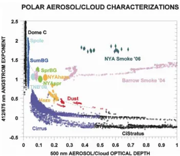
AOD, which is a result of their relative size, where particle size is inversely proportional to a parameter referred to as the ˚Angstrom exponent ( ˚A). ˚A is quantified as the negative slope of the spectrally varying AOD when plotted on a log scale (Stone, 2002). Figure 7 illustrates how the different aerosol types can be classified by plotting ˚A (derived from the 412/675 nm pair of wavelengths) as a function of AOD at 500 nm for data measured at different remote sites. Points falling near the bottom and to the right on the scatter plot have larger particle size and greater opacity than those at the upper left. Pristine conditions at Dome Concordia (Dome C) and South Pole (Spole) have the lowest values of AOD and the particles are relatively small, whereas dust particles tend to be larger and more opaque. Typical Arctic haze falls in between these extremes as evidenced in data collected at Barrow, Alaska and at Ny- ˚Alesund during spring. Smoke from boreal forest fires during 2004 in Alaska was observed to be invariant in size while having a wide range of optical depths. A similar signature was observed for the May 2006 smoke episode at Ny- ˚Alesund, which shows the same flat feature in the plot but at a higher value of ˚A. This suggests that the plume contained high number of aerosols in the ac-cumulation mode. This is corroborated by chemical analyses (Sect. 4.2) and by model simulations of Stohl et al. (2007) which indicate that plume was composed of a mixture of biomass burning smoke and small particles produced by fos-sil fuel combustion.
4.2 AOD derived from MERIS satellite observations To gain information on the spatial distribution of the plume MERIS satellite measurements were examined for the pe-riod of interest. AOD was estimated and compared with the photometric observations made at Ny- ˚Alesund. Unfor-tunately, retrieval methods developed to date are not appro-priate for polar applications. The algorithm works best when the target area (surface) is dark and for the regions within +/−60◦of latitude as described in Kaufman (1997) and von Hoyningen-Huene et al. (2003, 2006). The “spectral inter-correlation technique” fails at high latitudes and over bright surfaces, such as bare soils, snow or ice. Existing look up tables (LUTs) not adequately resolve aerosol effects over bright surfaces.
Thus, for this investigation we utilize a method referred to as the Bremen Aerosol Retrieval (BAER) (von Hoyningen-Huene et al., 2003, 2006, 2007) to evaluate the dispersion and opacity of the smoke plume by observations of MERIS. The MERIS instrument on board of ENVISAT measures well cal-ibrated top of atmosphere radiance in 15 channels, between 0.412–0.900 µm and a bandwidth of 10 nm. Reduced resolu-tion data near real time data have been used, having a ground resolution of 1.2×1.2 km2.
The swath width is 1.100 km. Generally BAER separates top-of atmosphere reflectance, measured by a satellite in-strument into the surface and the atmospheric fraction,
us-Figure 7. Plot of Ångström exponents as a function of 500 nm aerosol optical depth. Clusters
Fig. 7. Plot of ˚Angstr¨om exponents as a function of 500 nm aerosol optical depth. Clusters of points correspond to one-minute data with exception of points labelled NYAspr, which represents a mean for Ny- ˚Alesund during spring. The dashed curve is a best fit of all the data, excluding boreal smoke. Particle size is inversely related to the ˚Angstr¨om exponent. From left to right, Dome C and Spole represents pristine conditions at Dome Concordia and at South Pole, Antarctica with other clusters representing summer and spring background (BG) conditions, Arctic haze, Asian dust, and cirrus cloud at Barrow, AK, respectively. Smoke, made up of small particles, has a distinctive signature that is invariant over a range of AOD. Grey diamonds are hourly average data for the May 2006 event at Ny- ˚Alesund, which represents a mixture of biomass smoke and anthropogenic pollutants.
ing surface reflectance models, tuned from the spectral satel-lite measurements. The aerosol reflectance will be obtained from the atmospheric fraction, subtracting Rayleigh path reflectance and correction of transmittance of gaseous ab-sorbers (ozone in the spectral channels of 0.510–0.665 µm). The approach has been extended for Arctic conditions, con-sidering a pseudo spherical atmosphere for large zenith dis-tances. Thus airmass factors based on Kasten and Young (1989) have been used instead of that of a plane parallel at-mosphere.
A look up table (LUT) was developed on the basis of a phase function from LACE-98 (von Hoyningen-Huene et al., 2003) assuming a single scattering albedo (SSA)=1.0. This assumption is nearly valid for typical aerosols observed over Europe and also is in good agreement with AERONET mea-surements (Holben et al., 1998, von Hoyningen-Huene et al., 2006). As described in Sect. 4.2 the absorption of the aerosol observed in Ny- ˚Alesund is high. Although the absolute con-centrations of light-absorbing particles were high during the plume event the mass fraction of Elemental Carbon (EC), as will be shown below, was only a few percent. We will further show that there is a very strong effect of relative humidity
on the aerosol extinction. The water uptake by the aerosol again increases the SSA. Thus the real SSA is smaller than 1; however, larger than a value, obtained for dry aerosol. The unknown and therefore neglected real value for the SSA in the retrieved AOD from MERIS observations can lead to an underestimation of AOD within the haze plumes up to 30% depending on SSA. This may explain the deviations between the retrieved AOD from MERIS and the observations at
Ny-˚
Alesund. Outside the plume the assumption of less absorb-ing aerosol is justified and leads to AOD comparable with ground-based measurements although the AOD from satel-lite (∼0.4 at 442 nm) is for example around 33% less com-pared to the measurements in Ny- ˚Alesund (∼0.6 at 442 nm) for 2 May 2006. The BAER approach separates the con-tribution of the surface reflectance from the atmospheric re-flectance using land and ocean surface models. These cover only darker ground reflectance. Snow and ice cover are too bright for a separation of aerosol effects and will be removed from the retrieval by the cloud screening, described below. Thus, AOD retrievals by BAER in the Arctic can be per-formed only over snow and ice free areas, e.g. open water regions.
A further complication in using the MERIS data to study aerosol is the need to distinguish them from clouds. The screening algorithm in common use would identify thick aerosol as cloud and thus eliminate valid plumes. An im-proved cloud-screening algorithm was thus developed, which implements a three-stage approach to identify aerosols. First, the reflectance limits of three shortwave channels were set to ρTOA=0.2, a value exceeded is assumed to be cloudy. The threshold is based on the minimum cloud reflectance, given by (Kohkanovsky and Rozanov 2003; Kohkanovsky 2006). Second, pixels having a ratio of
ρ1(0.412 µm)/ρ2(0.443 µm)<1.08 between the blue chan-nels were eliminated as being cloudy because they have a significantly reduced Rayleigh scattering component com-pared to aerosols with a transmission down to the ground. Third, clouds are more inhomogeneous. Therefore, the spa-tial variability within a 5×5 pixel masque is used to distin-guish aerosol from cloud. As criterion the ratio between the standard deviation σ5×5 and the mean of the derived optical depth AOD5×5, R=σ5×5/AOD5×5 is used. In the case R is greater than a value B clouds are assumed to be present. B is also dependent on the optical depth itself, wherein for high values of AOD B must be set lower because the probability that clouds exist increases. For high AOD B=0.1 is used.
For long range transports of strong pollution events, like in this smoke episode, all three criteria deviate from nor-mal aerosol within the planetary boundary layer. The smoke gives strongly increased aerosol reflectance, partly exceeding the minimum cloud reflectance. Its height extension of the main plume is 2 km with additional layers above lead also to a relative reduction of observed Rayleigh scattering. Fur-ther the plume is more variable. Therefore, over the source region in western Russia and during the transport to
Sval-bard the strongest parts of the plume are identified partly as clouds.
Figure 8 presents the results of the MERIS analysis for the period from 1 to 4 May 2006. We are able to resolve the higher AOD over the source region and the extension of the plume towards Svalbard on 2 May 2006, demonstrating the potential of the satellite products now available. The loca-tion of highest AOD in the imagery is in very good agree-ment with the highest CO concentrations measured with the AIRS instrument (Stohl et al., 2007). While these are gratify-ing comparisons, it is clear that further improvements to the cloud-screening and retrieval algorithms are needed for polar applications in order to make the best use of global satellite coverage.
4.3 Chemical and micro-physical aerosol characteristics measured at Ny- ˚Alesund
The chemical and microphysical characterisation of the aerosols is important for the radiative transfer calculations in Sect. 5. The model used within this study relies only on the measured size distribution and the chemical composition at Mt. Zeppelin. In order to derive aerosol optical proper-ties for the vertical atmospheric column this section will be used to estimate these input values for the model described in Sect. 2. As shown above the smoke plume has not been vertically mixed and the airmasses at different levels are well separated, making it likely that the aerosols in these layers are different. This approach was in fact also used success-fully within the study published by Treffeisen et al. (2005). 4.3.1 Aerosol size distribution measurements
The aerosol number density and size distribution is measured using a TSI 3010 Condensation Particle Counter (CPC), a Differential Mobility Particle Sizer (DMPS) using a cus-tom built differential mobility analyser coupled to a TSI3010 CPC, and an Optical Particle Counter (OPC) model Grimm 1.001. The CPC has a nominal cut-off at 10 nm diame-ter and thus measures the total number density for particles larger than approximately 10 nm. The OPC observes par-ticles larger than 0.35 µm diameter. Although the instru-ment can normally provide six size classes between 0.35 and 6.5 µm, the setup during the plume event was to store only integral number density for particles larger than 0.35 µm. The DMPS system scan between 10 and 900 nm diameter, but data for particles smaller than approximately 15 nm and larger than about 700 nm should be taken with care. The small size range is affected by bit resolution limitations in the data acquisition system. The larger size range is affected as charge correction is initiated by extrapolating the obser-vations to larger sizes and by not excluding large particles using a cyclone. A Fuchs charge distribution is assumed for the inversion (Wiedensohler, 1988).
Figure 8. Regional pattern of the retrieved and cloud screened AOD for 0.443 µm (channel 2)
Fig. 8. Regional pattern of the retrieved and cloud screened AOD for 0.443 µm (channel 2) derived from MERIS observations using BAER
algorithm for 1 May (left upper panel), 2 May (right upper panel), 3 May (left lower panel) and 4 May 2006 (right lower panel). Each plot of one day is composed by three orbits (between 08:00 and 12:00 UTC) containing three scenes of 4 minute data. Thus the area between 85◦N and 53◦N and 10◦W and 35◦E has been covered. The AOD in the overlap region of the orbits is the average of the 2 or 3 observations within the observation times.
Despite uncertainties at both ends of the size distribution we choose to use the full range rather than to fit data using lognormal parameters. Ideally the integrated number density based on the size distribution should be equal to or less than that observed by the CPC. This comes from the used cut-off characteristics of the CPC’s and the size range used for the DMPS system. In the absence of small particles (∼20 nm)
the ratio should be very close to one. With an increasing number density of particles around the cut-off of the CPC (10 nm), this ratio will decrease as the DMPS system will not detect these particles with the same efficiency. The av-erage ratio between the integral number densities calculated from the size distribution divided by the total number densi-ties observed by the CPC was 0.74 for the five week period
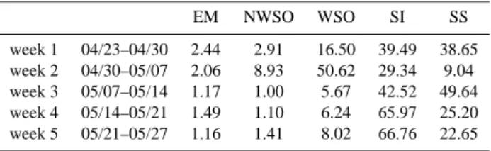
Table 1. Relative contributions of different components necessary
for the model input as obtained by measurements of chemical com-ponents and particle size distribution in Ny- ˚Alesund. EM = ele-mental carbon; NWSO = non-water-soluble organic matter; WSO = water-soluble organic matter; SI = water soluble inorganic matter; SS = sea-salt. EM NWSO WSO SI SS week 1 04/23–04/30 2.44 2.91 16.50 39.49 38.65 week 2 04/30–05/07 2.06 8.93 50.62 29.34 9.04 week 3 05/07–05/14 1.17 1.00 5.67 42.52 49.64 week 4 05/14–05/21 1.49 1.10 6.24 65.97 25.20 week 5 05/21–05/27 1.16 1.41 8.02 66.76 22.65
(see Table 1 for the specific dates) investigated in this study. This is expected as in May particle production events are fre-quent. The average ratio during the 2 to 3 May 2006 was 0.99. During this period there were almost no small particles present at all. Comparison of the average ratios based on in-tegral values over the relevant size range derived from the DMPS divided by the number density observed by the OPC gives a value of 0.93 for the entire period and 0.91 for the 2 and 3 May 2006. This is within the uncertainty of the OPC sample flow.
4.3.2 Absorption measurements
Aerosol particle light absorption is measured using a cus-tom built instrument which is operated using the same filter substrate and principles as the commercial Particle Absorp-tion Soot Photometer sold by Radiance Research. The in-strument uses one light source (525 nm) and two detectors to compensate for lamp drift. A filter enhancement correction of 2 is used. The uncertainty in the data is rather high and can be as high as a factor of two. These data will be used to compare with the calculated absorption coefficients based on the observed size distribution and chemical composition. To initiate calculations an independent observation of elemental carbon will be used.
4.3.3 Chemical measurements
Elemental and Organic Carbon (EC and OC) is determined from weekly filter samples. Aerosol particles are col-lected on quartz fibre filters using a Leckel SEQ57/50 sam-pler where filters are automatically changed at 12:00 UTC on Sundays. Elemental carbon (EC) and organic carbon (OC) are determined using the NIOSH 5040 thermo-optical method (Birch and Cary, 1996). The sampling setup is mainly intended for determining EC and its design it not op-timal to measure OC. Due to the rather long storage time of the exposed filters before analysis (e.g. 14 weeks for the first filter obtained during the smoke event) and the way of storing the exposed filters in a stack, there is a risk that semi-volatile organic species are transferred between the different filters
by diffusion. Blank filters stored with the ambient samples are used to subtract a baseline. In the case of the most pol-luted week the OC baseline represented 2.5% of the amount analysed on the ambient sample, whereas the EC baseline represented less than 1.5%. In the case of the cleanest week the OC baseline represented almost 60% of the amount anal-ysed on the ambient sample, whereas the EC baseline repre-sented less than 15%. Thus, data should be taken by care, but it is the best information available to us. Time series of the temporal evolution are presented in Stohl et al. (2007) and will not be repeated here.
In addition to the weekly quartz filter sampling one high-volume quartz fibre filter was collected (intended for a fea-sibility study) between the 28 April and 3 May 2006. From this large filter several small punches were also analysed us-ing the thermo-optical method mentioned above. Some of these punches were exposed to water in order to dissolve wa-ter soluble organics prior to being analysed in the same way as the non-water treated samples. The difference in observed OC is used as an estimate of the partitioning into a water- and a non-water soluble fraction of OC. This estimate is based on one sample period only, but will be used in all calculations performed in this study. The organic fraction was found to be represented by ∼85% water soluble material and ∼15% water insoluble organics.
Inorganic species (Cl−, NO− 3, SO
2− 4 , Ca
2+, Mg2+, K+,
Na+, NH+4) were analysed using ion chromatography. Daily
samples are collected using open faced NILU filter holders, loaded with 47 mm diameter Teflon filter (Zefluor 2 µm). The species NO3− and NH+4 are reported as both particu-late and gaseous phase, which overestimates the contribu-tion from particles by about 10%. The ions are grouped into soluble inorganic matter (SI=NO−3, SO2−4 , NH+4), sea salt
(SS=Cl−, Mg2+, Na+). The remaining analysed ions K+
and Ca+will be added to the SI for the later radiation
calcu-lations. Temporal variation of the obtained numbers can be found in Stohl et al. (2007). Quantitative measurements of minerals and metals are not available.
An indication for the presence of mineral particles was found on a filter for carbon analysis covering the sampling period from 30 April to 7 May. This filter showed a pinkish colour residue on the filter even after being heated to almost 900◦C during the thermal-optical analysis. Normally even the blackest filters are white after the heating of the filter. Thus, parts of the filter were analysed in a scanning electron microscope using energy dispersive X-ray analysis (EDX). Many particles presented peaks in the energy spectra indi-cating composition of Al, Fe, Ca, K, but also Na, Cl and Mg were determined as filter components. An example of an iron rich particle mixed with sea salt is presented in Fig. 9 with its corresponding energy spectra. The large Si and O peaks are due to the filter media and the presence of S comes from the tape that holds the filter to the stub. Although we are unable to make a quantitative estimate on the amount of minerals
C KA O Ka NaKa MgKa AlKa SiKa S Ka K Ka CaKa FeKa 1.00 2.00 3.00 4.00 5.00 6.00 7.00 8.00 9.00 10.00 11.00
Figure 9: Result of filter analyzed in a scanning electron microscope using energy dispersive
2
A
v
r
g
rt
o
tr
to
[μ
g
Fig. 9. Result of filter analysed in a scanning electron microscope using energy dispersive X-ray analysis (EDX) for the period 30 April to 7
May 2006.
and metals, the SEM analysis is evidence of their existence at least during the second week analysed in this study.
As the model needs the relative mass contribution to per-form the radiation calculations we perper-formed a mass esti-mation with the chemical inforesti-mation obtained above. For this we sum up the chemical species and scaled the measured mass of EC with a factor of 1.1, and of OC with a factor of 1.8 in order to represent other atoms associated with elemental and organic carbon atoms. The particle mass concentrations obtained by summing up the mass of chemical species are then compared to the mass concentration estimates derived from the particle size distributions and assuming an average particle density of 1.5 g cm−3. The estimates are presented in Fig. 10. We note a good agreement between these two esti-mates. Except for the third week from 7 May to 14 May 2006 (39%) the relative difference is less than 18%. The particle mass (PM) estimated by the size distributions systematically under estimates the PM based on the chemical analysis. This is also evident in parameters of a linear regression between these two estimates, giving a slope of 1.00 and an intercept of −0.51. There may be several reasons for this difference. Firstly, the constant density used does not represent the real aerosol density measured and secondly, the fact that particles above about 1 mm are not accounted for in the size distribu-tion may influence the calculated mass. However, the main information from Fig. 10 is that there appears to be no sub-stantial PM not accounted for by the size distributions nor explained by chemical analysis.
Therefore the particle mass concentration estimated from size distributions and that based on the chemical analy-sis provide a conanaly-sistent picture, which gives confidence in the further analysis. The relative contributions for
elemen-0 2 4 6 8 10 12 A v e ra g e p a rt ic le m a ss c o n c e n tr a tio n [μ g /m 3] 1 2 3 4 5 Weekly samples
Figure 10. Average particle mass concentration for the sum of chemical estim
Fig. 10. Average particle mass concentration for the sum of
chemi-cal estimates (blue) and chemi-calculated by using the integral of the mea-sured size distribution at Mt. Zeppelin with an assumed aerosol den-sity of 1.5 g cm−3(red) as described in Sect. 4.2. The numbers for the weekly samples are explained in Table 1.
tal carbon matter (EM), non-water-soluble organic matter (NWSO), water-soluble organic matter (WSO), water solu-ble inorganic matter (SI) and sea-salt (SS) used in the radia-tion calcularadia-tions for each week are presented in Table 1. We note that the two first weeks (23 April to 30 April 2006 and 30 April to 7 May 2006) when the plume passed over Sval-bard present larger or much larger fractions of organic matter for both water and non-water soluble fractions. Week 7 May to 14 May 2006 show more SS than the other two non-plume
0.0 2.5 5.0 7.5 10.0 σabs (m -1) * 10 -6 04-23 04-24 04-25 04-26 04-27 04-28 04-29 04-30 week 1 0.00 0.25 0.50 0.75 1.00 σabs (m -1) * 10 -6 05-07 05-08 05-09 05-10 05-11 05-12 05-13 05-14 week 3 0.00 0.25 0.50 0.75 1.00 σabs (m -1) * 10 -6 05-21 05-22 05-23 05-24 05-25 05-26 05-27 05-28 week 5 0 5 10 15 20 25 σabs (m -1) * 10 -6 04-30 05-01 05-02 05-03 05-04 05-05 05-06 05-07 week 2 0.00 0.25 0.50 0.75 1.00 σabs (m -1) * 10 -6 05-14 05-15 05-16 05-17 05-18 05-19 05-20 05-21 week 4
Fig. 11. The figure shows the observed and calculated absorption coefficients for the five weeks for which average bulk chemistry is estimated
(see Table 1). The dots are hourly averaged absorption coefficients observed by the custom built PSAP. The red and blue lines are calculated absorption coefficients assuming an internally and externally mixed aerosol, respectively. Note that the scales of the different panels are very different as data range over several orders of magnitude. The numbers for the weekly samples are explained in Table 1.
weeks 14 May to 21 May 2006 and 21 May to 27 May 2006, which could be an indication of the reason for the relatively larger difference between the estimated PM that week as dis-cussed above. In the current study, we do not know whether the aerosol predominantly is internally or externally mixed as the chemical analysis performed above cannot provide infor-mation on the mixing state. Previous investigations have sug-gested that calculation of radiative effects of Arctic aerosols are very sensitive to the mixing state and some studies point to an internally mixed state (Hara et al, 2003; Treffeisen et
al., 2005), whereas other studies indicate external mixtures (Heintzenberg and Covert, 1987). Therefore we investigated which mixing state most likely dominated the aerosol during the smoke event.
For this we calculated the absorption of the dry aerosol us-ing the weekly estimated bulk chemistry from Table 1 and the hourly averaged size distribution from the DMPS by us-ing the MIEV0 code (Wiscombe, 1979) to determine the ab-sorption coefficients and compared these calculated values to the measured absorption coefficients at Zeppelin Station.
The results are presented in Fig. 11. Note that the scales of the different panels are very different as data range over several orders of magnitude. In general the observed absorp-tion coefficient is between or very close to either of the two assumed aerosol mixing states (external and internal mix-tures). The main exception is during the plume events at the beginning of May where both aerosol models overesti-mate the observed values. The model assumes a fixed chem-istry for a one week sampling period under consideration. Therefore, deviations between calculated and measured ab-sorption coefficients could either be the result of variation in chemistry, mixing state or a combination of both. As more detailed chemical information is not available for this study, we choose to explain the differences in terms of soot mix-ing state only. Shiftmix-ing between mixmix-ing states is particularly evident from 23 April to 30 April 2006 where the first two peaks of the absorption coefficient follow the internal mixing model, but throughout the remainder of the week the absorp-tion coefficients follow the model using an externally mixed aerosol. During the studied period, with the exception of week three, the observed absorption coefficient best repre-sented when the model calculations assume external mixing. This is highlighted by comparing the mean relative differ-ence for between measured and modelled absorption values assuming external and internal mixtures corresponding to 9% for the external mixture and −38% for the internal mixture.
5 Influence on heating rates
5.1 Derivation of vertical aerosol profile
For the following calculation we chose two days. One case is at 27 April 2006, which was most probably also influenced by fossil fuel combustion sources and one case at 2 May 2006, when the highest pollution was observed (see for detail Stohl et al., 2007). In order to represent the vertical structure of the aerosol for 27 April 2006 and 2 May 2006 we calcu-late the ambient extinction coefficient at 530 nm from their assumed composition, mixture and number size distribution. The size and composition of the aerosol is further adjusted for hygroscopic growth as described in Sect. 2.1. The rel-ative chemical composition obtained from the aerosol mea-surements is assumed constant in the whole vertical column. The approach also assumes that the shape of the size distri-bution is preserved in the entire column (i.e. that the relation between Aitken and accumulation mode remains the same, although the integral number varies). We further assume that no aerosol is present above 10 km.
The calculated vertical extinction profile is compared to the extinction profile observed by Lidar measurements at 532 nm in Ny- ˚Alesund. The Lidar system is well described in Ritter et al. (2004). In order to reproduce the vertical profile of extinction given by the Lidar we scale the vertical abun-dance of the aerosol by applying a height dependent scaling
factor. This scaling factor is always 1 at the level of mea-surements (i.e. 500 m) and below. Above 500 m, the scaling factor was allowed to vary between 0–1. By using an iter-ative approach, the abundance of the aerosol aloft was ad-justed until agreement between calculations and observations was achieved in terms of the extinction coefficient. The per-formance of the current approach was tested by comparing results derived with the methodology described in this study with data obtained with a different radiative transfer module at Svalbard during ASTAR2000 campaign (Treffeisen et al., 2005). The results indicate a very good agreement between the ASTAR2000 campaign and current calculations which was evident both from magnitude and vertical structure of the calculated heating rate (not depicted here).
The calculation of the extinction is very sensitive to am-bient RH. The hygroscopic growth factors (GF) of sea salt adopted from GADS agrees with GF of NaCl. The hygro-scopic behaviour of NaCl involves RH-hysteresis between
∼42–75% RH. In practice this means that the growth fac-tor (GF) of the sea-salt component always is assumed to be 1 below 42% RH. Above 75% RH, the sea salt fraction will always include water. However, if the RH is in-between 42% and 75%, the GF of the sea salt will depend on if the air is changing from a higher to a lower RH or vice versa, i.e. as-suming that the RH is decreasing or increasing. If subjected to an increase from initially low RH to higher RH, the par-ticles will not grow until the deliquescence point is reached. If instead the RH is decreasing from values above the deli-quescence point, the particles will contain water until the RH drops below the efflorescence point. This behaviour is called RH-hysteresis.
For the soluble organic and sulphate fraction of the aerosol we disregard the role of RH hysteresis and use the tabulated values of GF as given in the GADS dataset regardless of RH-history. For the organic fraction, this assumption most likely does not include a large error. It is however more uncertain whether or not the sulphate fraction of the aerosol exhibits hysteresis in the RH range in this study. This since we do not know if the sulphate is in the form of sulphuric acid, ammonium bisulphate or ammonium sulphate. Depending on which species we choose, the hygroscopic behaviour will differ. In the GADS data set used in this study, the GF’s of sulphate is comparable in magnitude with sulphuric acid.
For the calculation of the extinction profile we use the size distribution measurements coinciding with the observa-tion time period of the Lidar to allow for direct compari-son between calculated and observed extinction profiles. RH measurements are used from the routine soundings in
Ny-˚
Alesund. For the pollution situation of 27 April 2006 simul-taneous Lidar and size distribution observations were avail-able between 00:00–02:00. Since the soot fraction is best described as an external mixture, we define the base case conditions with an external mixture. Shown in Fig. 12 are the vertical extinction profiles derived using assumptions of either decreasing or increasing relative humidity.
0 0.01 0.02 0.03 0.04 0.05 0.06 0.07 0 1 2 3 4 5 6 7 8 9 10 Extinction coefficient (km−1) Altitude (km) Increasing RH Decreasing RH Observations
Figure 12: Calculated extinction profile at 530 nm at 27 April 2006 and estimaFig. 12. Calculated extinction profile at 530 nm at 27 April 2006 and estimated range of extinction coefficients assuming that the air is in a state of increasing or decreasing RH. Calculations and obser-vations cover a time interval between 00:00–02:00. See Sect. 5.1 for further details.
As can be seen in Fig. 12, the assumption of increasing RH results in lower extinction compared with the calculation as-suming decreasing RH. The measured extinction profile at 530 nm is added for comparison. It should be mentioned that since we assume an external mixture, the RH assump-tion does not affect the absorpassump-tion profile. The calculaassump-tions were repeated for the smoke day 2 May 2006 for the time interval 20:00 to 23:00. The result is shown in Fig. 13. The model extinction exceeds the observed extinction at the lower levels, both for calculations performed assuming decreasing and increasing RH. One probable cause for the deviation is the changes in RH in the air during the course of the day. The time for Lidar observations and balloon soundings does not coincide. At higher altitudes, however, there is good agree-ment between observed and modelled extinction. The de-rived vertical profile was evaluated by calculating the AOD followed by comparison with measured AOD (see Sect. 4.1). During the 27 April 2006 AOD measurements are avail-able from 03:00 to 09:00. The AOD were averaged and com-pared to calculated values using the average size distribution from the same time interval as the AOD measurements. The comparison considers two wavelengths, 500 and 1000 nm (see Table 2). The calculated values range from 0.19–0.29 at 500 nm, were the lower value correspond to the calcula-tions performed assuming increasing RH. The observed av-erage value was 0.186 (0.158–0.206, ±1 standard deviation). At 1000 nm, the calculated values ranged from 0.059-0.089. The observed AOD at 1000 nm was 0.075 (ranging from 0.07–0.081). The same comparison was repeated for 2 May 2006. The calculated optical depth at λ=500 nm range from 0.52–0.58, while the observed AOD was on average 0.507
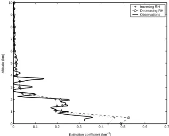
0 0.1 0.2 0.3 0.4 0.5 0.6 0.7 0 1 2 3 4 5 6 7 8 9 10 Extinction coefficient (km−1) Altitude (km) Incresing RH Decreasing RH Observations
Figure 13. Calculated extinction profile at 530 nm during 2 May 2006 and estimFig. 13. Calculated extinction profile at 530 nm during 2 May 2006 and estimated range of extinction coefficients assuming that the air is in a state of increasing or decreasing RH. Calculations and obser-vations cover a time interval between 20:00–23:00. See Sect. 5.1 for further details.
(0.412–0.603±1 standard deviation). At 1000 nm the model result in AOD ranging from 0.157–0.183, compared with av-erage observed AOD at 1000 nm of 0.157 (0.135–0.178). 5.2 Calculation of the change in daily heating rates due to
aerosols for 27 April and 2 May 2006
The heating rate is calculated at wavelengths of 0.25–4 mi-crons. The heating rate reported here is for aerosol contribu-tion only. That means that we subtract the calculated heating rate by the heating rate of a Rayleigh atmosphere. Twenty-four hourly heating rate profiles were calculated from mean size distribution during the day of interest, adopting the verti-cal profile derived in Sect. 5.1. The analysis considers the 27 April 2006 which was already influenced by smoke particles and the smoke episode represented by 2 May 2006. The cal-culations use the observed albedo for the two cases which is measured routinely in Ny- ˚Alesund. We assume a spectrally uniform surface albedo. The calculations assume clear sky conditions. For the base case conditions we assume an exter-nally mixed aerosol and that the air is in a state of increasing RH. This assumption does not directly affect the absorption coefficient, but has a small positive effect (a few percent) on the heating rate in the lower levels due to less scattering aloft. The calculated heating rates for 27 April 2006 are given in Fig. 14. The measured albedo during the 27 April 2006 was 0.72. The heating rate calculated for the daily mean size distribution peaked at 0.11 K day−1 at an alti-tude of 1 km. The range of heating rates for the exter-nal mixture assumption was calculated using the daily 25th and 75th percentiles of the size distributions. At the 1 km
Table 2. Calculated and measured AOD at 500 nm and at 1000 nm for days 27 April and 2 May 2006.
Calculated range Observed range Calculated range Observed range
at 500 nm at 500 nm at 1000 nm at 1000 nm 27 April 2006 0.19–0.29 0.158–0.206 0.059–0.089 0.070–0.081 2 May 2006 0.52–0.58 0.412–0.603 0.157–0.183 0.135–0.178 0 0.1 0.2 0.3 0.4 0.5 0.6 0.7 0.8 0 1 2 3 4 5 6 7 8 9 10
Daily average heating rate (K day−1)
Altitude (km)
Internally mixed aerosol, decreasing RH Externally mixed, increasing RH Externally mixed, 25th perc., increasing RH
Externally mixed, 75th perc., increasing RH
Figure 14: Vertically resolved calculated daily averaged heating rates (K day ) for 27 April Fig. 14. Vertically resolved calculated daily averaged heating rates
(K day−1) for 27 April 2006. The heating rate for the completely externally mixed case using the assumption of increasing RH for av-erage and 25th–75th percentiles of the daily size distributions. The upper limit is defined as completely internal mixture and decreasing RH.
altitude, the 25th percentile data resulted in a heating rate of 0.05 K day−1 and the 75th percentile resulted in a heat-ing rate of ∼0.15 K day−1. As a comparison we also calcu-lated the heating rate assuming that the soot is completely internally mixed in the aerosol. The result is also shown in Fig. 14. By assuming an internal mixture, the calculated heating rates increase significantly at all levels. The shape of the vertically distributed heating rates also reflects the ambi-ent humidity distribution since the soot fractions is dispersed in an aerosol that undergoes hygroscopic growth. The maxi-mum in heating rate is still at 1 km, but in the case of internal mixture the heating rate peaks at ∼0.75 K day−1.
The heating rates for 2 May 2006 are given in Fig. 15. The measured albedo was 0.65. The heating rate calculated for the daily average size distribution reached a maximum of 0.55 K day−1at 0.5 km altitude. The range of maximum heating rates in the case of external mixture derived from the 25–75th percentiles was 0.45–0.65 K day−1at 0.5 km al-titude. In the case of internal mixture, the heating rate peaked at roughly 1.7 K day−1at an altitude of 0.5 km. Overall, the heating rates calculated for the internally mixed aerosol are substantially larger. 0 0.2 0.4 0.6 0.8 1 1.2 1.4 1.6 1.8 0 1 2 3 4 5 6 7 8 9 10
Daily average heating rate (K day−1)
Altitude (km)
Internally mixed aerosol, decreasing RH Externally mixed, increasing RH Externally mixed, 25th perc., increasing RH Externally mixed, 75th perc., increasing RH
Fig. 15. Vertically resolved calculated daily averaged heating rates
(K day−1) for 2 May 2006. The heating rate for the completely ex-ternally mixed case using the assumption of increasing RH for av-erage and 25th–75th percentiles of the daily size distributions. The upper limit is defined as completely internal mixture and decreasing RH.
It is evident that the calculated heating rate is crucially de-pendent on the assumption of the mixing state. As in the case of 27 April 2006, the Mie-calculations indicated that the aerosol predominantly was externally mixed with respect to soot. This also applied for the 2 May 2006. However, it is not likely that the soot is completely externally mixed. Neither is it likely to assume that the aerosol is completely internally mixed. The aerosol is rather best represented by a combi-nation of internally and externally mixed soot fractions. In the case of internal mixture, we further also assume that the soot is evenly distributed over the entire size spectra. Given these assumptions, it is likely that the actual heating rates calculated for the two days is in between the minimum char-acterised by the external mixture assumption and the maxi-mum given by the assumption of the internal mixture. The difference in peak heating rates between external and inter-nal mixing states was more than a factor of 7 on 27 April and almost a factor of 3 on 2 May 2006.
Previous studies have reported aerosol induced heating rate of 0.76 K day−1during Arctic haze conditions for inter-nally mixed aerosols with a soot mass comparable in magni-tude to the current study (Wendling et al., 1985). Considering
0 0.1 0.2 0.3 0.4 0.5 0.6 0.7 0 1 2 3 4 5 6 7 8 9 10
Daily average heating rate (K day−1)
Altitude (km)
Albedo=0.64 Albedo=0.2 Albedo=0.9
Figure 16: Vertically resolved calculated daily averaged heating rates (K day ) for 2 May
Fig. 16. Vertically resolved calculated daily averaged heating rates
(K day−1) for 2 May 2006 assuming a surface albedo of 0.2, 0.64 and 0.9. Externally mixed aerosol and increasing RH conditions are assumed.
differences in season and mass of soot, the results are com-parable. Treffeisen et al. (2005) further report heating rate anomalies in the range of 0.3 K day−1in later studies of the heating rate during Arctic haze conditions.
5.3 Sensitivity of aerosol induced heating rate surface albedo
As an additional test we also investigated the sensitivity of the heating rate to changes in surface albedo. During the transport of the smoke in the Arctic it passes areas of al-ready open sea water having a low surface albedo and areas with snow/ice cover at the high altitudes with a high surface albedo. A high albedo will increase the heating rate due to more reflection from the surface. This test was performed during 2 May 2006 assuming an external mixture. Calcu-lations were performed assuming albedos of either 0.2 or 0.9. The result is shown in Fig. 16. The lower albedo re-sults in maximum heating rate of 0.43 K day−1at 0.5 km al-titude. The higher albedo results in a maximum heating rate of 0.64 K day−1 at the same altitude. It is thus evident that a proper representation of the surface albedo is necessary to represent the actual heating rates.
6 Conclusions
Late April anomalies in synoptic conditions established a pathway for the rapid transport of aerosols from fires in East-ern Europe to the Arctic. The transport is well described in Stohl et al. (2007) while this paper focussed on the radiative effects of this air pollution in the Arctic environment.
Surface observations show that the relation between the ˚
Angstrom exponent and optical thickness for the event pre-sented in this study is rather different from that observed for a forest fire plume over Barrow, Alaska. This is also true when comparing with dust and other spring time Arctic haze events. The ˚Angstrom exponent is large compared to these other plumes while presenting a high optical depth as well. We believe that differences are due to a mixture in aerosol characteristics. Indeed the smoke appears to be mixed with pollutants along path as shown by extensive chemical anal-yses from Mt. Zeppelin and transport analysis performed by Stohl et al. (2007). Considering the large relative abun-dance of organic species, and thus assumed lower hygro-scopic growth factors, this could explain the large ˚Angstrom exponent.
Comparison of AOD values from space and from the surface in the Arctic region show the difficulties in deal-ing with bright surfaces and cloud screendeal-ing and demon-strate the urgent need to develop specific algorithms for high latitude regions in order to make use of the satellite data. AOD from ground-based measurements (AOD∼0.6 at 442 nm) are around 33% more compared to satellite measure-ments (AOD∼0.4 at 442 nm) for 2 May 2006. Thus, espe-cially retrieval algorithms, working over snow and ice areas are urgently required. Nevertheless, the AOD from satellite showed the horizontal extension of the plume.
Calculated absorption coefficients based on the observed size distribution and chemical composition agree best with observed values when assuming a more externally mixed aerosol. The resulting heating rates depend strongly on the assumed mixing state of the aerosol. The difference in peak heating rates between external and internal mixing states was more than a factor of 3 on 27 April and almost a factor of 7 on 2 May 2006.
The radiative effect of the aerosol is very sensitive to changes in the relative humidity and the albedo. As the plume is transported from low latitudes all of these character-istics change. With time the plume will become more inter-nally mixed from coagulation and condensation. During the transport of the plume north the temperature decreases and the relative humidity increases. As the plume moves from over the open ocean to over the pack ice, the surface condi-tions will change dramatically. All of these three factors, ag-ing of the aerosol, increase in relative humidity, and increase in albedo act to enhance the heating rates in the plume.
To understand and assess the impact of these plume events requires detailed knowledge of the aerosol properties, their state of mixing, refractive index, and growth factors. Beside intensive measurements from ground, also satellite data will be necessary to follow the dispersion which is necessary for model simulation and their validation in future.