Global climate imprint on seismic noise

HAL Id: hal-00723544

https://hal.archives-ouvertes.fr/hal-00723544

Submitted on 9 Jun 2017

HAL is a multi-disciplinary open access archive for the deposit and dissemination of sci-entific research documents, whether they are pub-lished or not. The documents may come from teaching and research institutions in France or abroad, or from public or private research centers.

L’archive ouverte pluridisciplinaire HAL, est destinée au dépôt et à la diffusion de documents scientifiques de niveau recherche, publiés ou non, émanant des établissements d’enseignement et de recherche français ou étrangers, des laboratoires publics ou privés.

To cite this version:

Eléonore Stutzmann, Martin Schimmel, Geneviève Patau, Alessia Maggi. Global climate imprint on seismic noise. Geochemistry, Geophysics, Geosystems, AGU and the Geochemical Society, 2009, 10 (11), pp.Q11004. �10.1029/2009GC002619�. �hal-00723544�

Global climate imprint on seismic noise

Ele´onore Stutzmann

Institut de Physique du Globe de Paris, F-75252 Paris CEDEX 05, France (stutz@ipgp.jussieu.fr)

Martin Schimmel

Institute of Earth Sciences Jaume Almera, CSIC, E-08028 Barcelona, Spain

Genevie`ve Patau

Institut de Physique du Globe de Paris, F-75252 Paris CEDEX 05, France

Alessia Maggi

Institut de Physique du Globe de Strasbourg, UMR 7516, Universite´ de Strasbourg, CNRS, 5 rue Rene´ Descartes, F-67084 Strasbourg CEDEX, France

[1] In the absence of earthquakes, oceanic microseisms are the strongest signals recorded by seismic stations. Using the GEOSCOPE global seismic network, we show that the secondary microseism spectra have global characteristics that depend on the station latitude and on the season. In both hemispheres, noise amplitude is larger during local winter, and close to the equator, noise amplitude is stable over the year. There is an excellent correlation between microseism amplitude variations over the year and changes in the highest wave areas. Considering the polarization of the secondary microseisms, we show that stations in the Northern Hemisphere and close to the equator record significant changes of the secondary microseism source azimuth over the year. During Northern Hemisphere summer, part or all of the sources are systematically located farther toward the south than during winter. Stations in French Guyana (MPG) and in Algeria (TAM) record microseisms generated several thousand kilometers away in the South Pacific Ocean and in the Indian Ocean, respectively. Thus, secondary microseism sources generated by ocean waves which originate in the Southern Hemisphere can be recorded by Northern Hemisphere stations when local sources are weak. We also show, considering a station close to Antarctica, that primary and secondary microseism noise amplitudes are strongly affected by changes of the sea ice floe and that sources of these microseisms are in different areas. Microseism recording can therefore be used to monitor climate changes.

Components: 5366 words, 7 figures.

Keywords: seismic noise; microseisms; seismology.

Index Terms: 7255 Seismology: Surface waves and free oscillations; 7299 Seismology: General or miscellaneous. Received 11 May 2009; Revised 28 July 2009; Accepted 17 September 2009; Published 5 November 2009.

Stutzmann, E., M. Schimmel, G. Patau, and A. Maggi (2009), Global climate imprint on seismic noise, Geochem. Geophys. Geosyst., 10, Q11004, doi:10.1029/2009GC002619.

G

3

G

3

Geochemistry

Geophysics

Geosystems

Published by AGU and the Geochemical Society AN ELECTRONIC JOURNAL OF THE EARTH SCIENCES

Geochemistry

Geophysics

Geosystems

1. Introduction

[2] Seismic noise spectra display two peaks in the

period band 5 –25 s which are called primary and secondary microseisms. These microseisms are predominantly Rayleigh waves [Haubrich and McCamy, 1969] and they are recorded by all seismic stations whatever their location, on con-tinents, on islands [e.g., Stutzmann et al., 2000] and even on the seabed [Stutzmann et al., 2001]. The primary microseisms (period 10 – 20 s) are generated when ocean gravity waves reach shallow water near the coast and interact with the sloping seafloor [Hasselmann, 1963]. These seismic waves have periods similar to the incident ocean gravity waves. The secondary microseisms are generated by the interaction of two ocean gravity waves of similar periods that travel in opposite directions. When these ocean waves meet, they generate standing pressure fluctuations at the ocean bottom through a nonlinear mechanism [Longuet-Higgins, 1950]. The pressure fluctuations have half the period of the ocean waves and are the source of the secondary microseisms. The longest periods of the secondary microseisms can be attributed to very large storms, and the steep slope of the noise spectrum above 10 s period is due to the rarity of oceanic waves with periods greater than 20 s [Webb, 1998]. Recently, modeling of the deep ocean non-linear wave-wave interaction in a source region between the Labrador Sea and Iceland showed an excellent agreement with the secondary microseism amplitude recorded by stations in North America and Western Europe [Kedar et al., 2007], demon-strating the validity of Longuet-Higgins’s theory. [3] Friedrich et al. [1998] first used two arrays in

Northern Europe to locate the secondary micro-seism sources. They found a stationary source close to the coast in the Norway Sea that was independent of the oceanic storm location. Second-ary microseisms recorded by stations further South in Europe in December 2005 and January 2006 have been associated with both coastal and pelagic sources in the Mediterranean Sea [Chevrot et al., 2007]. Bromirski et al. [1999] and Bromirski and Duennebier [2002] showed that the secondary microseisms recorded by near coastal stations in the western United States are predominantly gener-ated by ocean wave-wave interactions at the nearest coastlines. Stehly et al. [2006] cross-correlated sev-eral years of noise and concluded that the California network records secondary microseisms whose source direction is stable over the year toward the Pacific Ocean. Gerstoft and Tanimoto [2007]

primary microseisms are generated near the coast whereas excitation of secondary microseisms occurs in a wider area, which confirms a different genera-tion mechanism for the two microseisms.

[4] All these regional studies confirm the oceanic

location of microseism sources, but the debate on secondary microseism source locations is still open. In this paper we investigate variations of the secondary microseism spectrum and of its direction of polarization at the global scale, and we show that these variations are related to changes in the source location over the year. We also show that the microseisms recorded by a station close to Antarctica are strongly affected by the ice cover variations nearby.

2. Data and Method

[5] In order to study seasonal variations of the

secondary microseisms we have considered the amplitude spectrum variations over many years and the polarization of the seismic signal for the year 2006.

[6] We have processed 15 years of continuous data

recorded by the global network of broadband seismic stations GEOSCOPE. Daily seismic noise levels were computed for the 27 stations of the network over the years 1992 to 2007. For each station, a robust power spectrum estimate was determined over sequences of 24 h using the method of Chave et al. [1987]. Data were win-dowed using prolate tapers. Time windows were selected so that they overlap by 50%. An iterative algorithm was used in order to eliminate earth-quakes or glitches as long as they do not exceed 20% of the length of the window. Fourier trans-forms of each time window were then computed and smoothed. The energy spectrum was computed over all data windows by using the median. The power spectral density estimate was then corrected by removing the instrumental response and con-verted into decibels (dB) with respect to accelera-tion. Averaging the spectra over 24 h of signal enabled us to obtain noise levels that are, for most days, similar to those obtained after careful selec-tion of signal sequences without earthquakes. [7] We also computed the polarization of the

secondary microseisms. As microseisms are pre-dominantly fundamental mode Rayleigh waves, they have elliptical retrograde polarization when recorded by stations located on rocky ground [Tanimoto and Riveira, 2005; Tanimoto et al.,

2006]. Using the 3 components of the seismogram, we have determined the semimajor and semiminor axes of the ellipse that best fits the ground motion. The eigenanalysis of the time-frequency represen-tation of the three components enables us to determine the back azimuth of the Rayleigh waves as a function of time and frequency as well as the degree of polarization [Schimmel and Gallart, 2003, 2004]. The degree of polarization is a mea-sure of the stability of the polarization in a partic-ular state with time.

[8] Noise spectra analyses are presented in section 3

and the polarization directions are discussed in section 4.

3. Seasonal Variations of the Noise

Spectrum Amplitude

[9] Figure 1a shows the noise level variations over

one year in the period band 0.1 – 50 s for the 27 stations of the GEOSCOPE network. Noise diagrams are plotted at the corresponding station location. Besides individual station site character-istics due to different geological settings, the main differences between the noise amplitude recorded by the different stations are due to the stations being located on continents, close to the coast or on

islands [Stutzmann et al., 2000]. Figure 1 (and Figure A1) clearly show that stations located on islands display higher noise amplitudes than con-tinental stations. Among island stations, there is no significant dependence of the maximum amplitude on the ocean in which the station is located. The maximum amplitudes range between 110 and 100 dB and the corresponding periods are between 4 and 6 s.

[10] Figure 1b shows a map of significant wave

height averaged over one year [Rascle et al., 2008]. We expect the strongest sources of microseisms to be in the oceans that record the highest ocean waves, though we do not look for the exact location of conversion of ocean waves into seismic waves. Swells may propagate long distances from the storms before generating microseisms either in deep or shallow water, but the microseism gener-ation areas, even if far from the storms, are likely to be in the same ocean. The microseism amplitude recorded by a given station is a function of the amplitude of the source and of the distance of propagation between the source and the station, as Rayleigh waves are attenuated during their propagation. Then, stations in the South Atlantic and South Indian Oceans should record the largest microseism amplitudes. This is observed for the five Southern Hemisphere island stations TRIS,

Figure 1. (a) Seismic noise amplitude variations over 1 year in dB with respect to acceleration. Noise diagrams are plotted at the corresponding station locations. The horizontal axis corresponds to days from 1 to 365, and the vertical axis is the period from 0.1 to 50 s using a logarithmic scale. (b) Significant wave height [Rascle et al., 2008] averaged over 1 year.

Geochemistry Geophysics Geosystems

G

3

amplitudes in the Northern Hemisphere compared with the Southern Hemisphere are also well corre-lated with the lower noise levels recorded by continental stations in the Northern Hemisphere (SSB, ECH, WUS) compared with continental stations in the Southern Hemisphere (PEL, SPB, CAN), an effect that is particularly visible during local summer.

[11] For stations at high latitude, whatever their

location, we clearly observe seasonal variations of the secondary microseism amplitude and period range. In the Northern Hemisphere, stations in the North Atlantic (KIP), North America (SCZ), Europe (SSB, ECH), China (WUS) and Japan (INU) show minimum amplitudes of the secondary microseism in July and August during local sum-mer. Closer to the equator, stations display no significant changes of the secondary microseism over the year, as can be observed for stations in Central America (UNM, HDC, MPG), West Indies (FDF), Africa (TAM) and in the Pacific Ocean (TAOE and PPT). Stations located in the Southern Hemisphere show maximum microseism ampli-tudes in July and August during local winter. These maximum amplitudes are particularly striking for the stations in the South Atlantic Ocean (TRIS), Indian Ocean (CRZF, RER, AIS, PAF) and Australia (CAN), and slightly less visible in South America (PEL and SPB).

[12] Figures 2a and 2b summarize the correlation

between maximum microseism amplitudes and local autumn and winter at high latitudes, and show that the latitude dependence of microseism amplitudes is repeated every year. We observe a good global temporal correlation between variations of the microseism amplitude and changes of the highest wave area averaged by longitude (Figure 2c). Thus, we expect the strongest sources of secondary microseisms to be located in the oceans around Antarctica during July and August, and in the North Pacific and Atlantic oceans during January and February. We note that even during Northern Hemi-sphere local winter, we still observe high ocean waves around Antarctica and therefore this area may be a source of strong microseisms over most of the year. This is consistent with the high ampli-tudes observed for stations in the Indian Ocean (PAF, AIS, CRZF) all year round.

[13] Figure 2 also shows that the lowest frequencies

of microseisms are excited during the respective winter months. During winter, the number of storms that induce higher-amplitude lower-frequency

on the right panel of Figure 2 indicates that a broader latitude area is affected by large storms during winter. The maximum period of the secondary microseism is related to half the period of the ocean waves, which explains the good correlation between high microseism amplitude at long periods and the area of large storms during local winter.

[14] For stations close to the equator such as HDC,

we observe no microseism amplitude variations. The absence of variations might be explained by negligible seasonal changes close to the equator, and by the fact that these stations are at similar distances to high ocean wave areas at high latitudes in the Northern or Southern Hemisphere. Indeed, ocean waves may travel long distances before generating microseisms [Gerstoft and Tanimoto, 2007].

[15] Although it is not the main topic of this paper,

we note that the two stations ECH (France) and HDC (Martinique Island) in Figure 2 also display noise level variations for periods smaller than 1 s. Furthermore, 1 day per week, we observe a thin line of lower amplitude. This is observed for most GEOSCOPE stations and corresponds to Sunday for most stations and to Friday for the station in Algeria (TAM). This decrease of noise can easily be associated with the drop of human activity 1 day per week, depending on the official religion of the country. It is not observed at the station PAF and neither at the other stations located on very small islands with little human activity (TRIS, AIS, CRZF).

4. Seasonal Variations of the Noise

Polarization Direction

[16] In order to confirm the relationship between

the secondary microseism amplitude variations and changes of the highest wave areas, we have com-puted the polarization of the seismic noise in the period band 5 –10 s. As secondary microseisms are predominantly fundamental mode Rayleigh waves, they have elliptical retrograde polarization when recorded on rocky soil, as it is the case for all GEOSCOPE stations [Tanimoto and Riveira, 2005]. A polarization analysis has been performed for January –February and July – August of 2006 following the procedure described in section 2. We counted for each month the occurrence of ellipti-cally polarized signals in frequency and back azimuth bins. Figure 3 shows the largest occur-rence of polarized signals as a function of azimuth

and frequency for 9 stations. On each plot, the radius corresponds to the frequency from 0.1 to 0.2 Hz and the azimuth is given by the angle. Green and red colors correspond to contours of the maximum number of polarized signals for January– February and July – August, respectively. For each month, the maximum number of polarized signals has been normalized to 1, and we have plotted contours above 60%, thereby showing the azimuth and frequency of the most abundant sources of secondary

micro-seisms. These source azimuths are then plotted at the station location in Figure 3d, in green for January – February and in red for July – August. For all 9 stations, the source azimuths are predominantly toward the closest ocean, but we observe azimuth variations between winter and summer.

[17] The three stations in Figure 3a are in the

Northern Hemisphere. At station ECH in France, the source azimuth is predominantly toward the

Figure 2. (a) Seismic noise amplitude variations over 2 years, 2003 and 2006, in dB with respect to acceleration for stations in the Northern Hemisphere (ECH), close to the equator (HDC), and in the Southern Hemisphere (PAF). (b) Sketch of seismic noise amplitude variations as a function of seasons. (c) Significant wave height [from Rascle et al., 2008] averaged over longitude as a function of Julian days. Latitudes of the three stations ECH, HDC, and PAF are marked with dashed lines for comparison.

Geochemistry Geophysics Geosystems

G

3

Atlantic Ocean both in winter and summer (Figure 3d) but in winter the southernmost source azimuth is N150W, whereas in summer we also observe source azimuths further South between N150W and N210W. The station in Japan (INU) shows source azimuths toward the Pacific Ocean

all year round, but the sources are toward the North Pacific during local winter and toward the South Pacific during local summer (Figure 3). The station in Hawaii (KIP), in the middle of the North Pacific Ocean, displays source directions toward the North from W to E in winter, and sources from all

Figure 3. Directions of the secondary microseism sources for nine stations in 2006. (a) Stations in the Northern Hemisphere, (b) stations close to the equator, and (c) stations in the Southern Hemisphere. For each diagram, the angle is the station back azimuth (azimuth of the source recorded at the station), and the radius corresponds to frequency between 0.1 and 0.2 Hz. Contours correspond to the maximum number of polarized signals per month, for months January and February in green and July and August in red. (d) Geographical map showing at the station location (black circles) the azimuths of the most abundant sources of secondary microseisms for months January and February in green and July and August in red.

azimuths including South in summer. Thus, for these three Northern Hemisphere stations, micro-seism sources are predominantly in the Northern Hemisphere during January– February, whereas in summer source azimuths are also or only (depend-ing on the station) further toward the south. This suggests that at least at station KIP and INU we detect secondary microseisms which have been generated by swells that originate in the Southern Hemisphere. For the station ECH in France, the southern directions may be associated with sources in the Mediterranean Sea or with sources further away, as there are very few large storms in the Mediterranean Sea during summer.

[18] For the three stations close to the equator

(Figure 3b), we observe similar seasonal variations. Station HDC is in Costa Rica at similar distances from the Atlantic and Pacific oceans. The source directions are toward both oceans with more sources toward the South Atlantic in July– August than in January – February. Station MPG in French Guyana is located 7 km away from the Atlantic Ocean coast. In January –February, this station displays source azimuths toward two directions: N and S-W (green contours in Figures 3a – 3c). The North direction points toward the nearby North Atlantic Ocean but there is no ocean in the vicinity of the station along the S-W direction (Figure 3d). In July – August, MPG station records source azimuths only toward South to West directions (red contours in Figures 3a– 3c). The coast along the S-SW direction is in Chile at a distance of about 3000 km from the station. Thus MPG station records microseisms generated in the South Pacific Ocean either at the Chile coast or further away.

[19] The third station (TAM) is in Algeria and in

winter it records microseisms that come from 3 azimuths: N-W, S-E and S (green contours in Figures 3a –3c). Along these azimuths, the closest coasts are in the Mediterranean Sea and the Atlantic Ocean. In July –August, all microseisms come from the S-E to S-W directions. Among these directions, the nearest coast corresponding to the azimuths N140E to N170E is in South Africa at a distance of more than 6000 km. Microseisms propagating along these azimuths are generated in the Indian Ocean.

[20] Both stations MPG and TAM record

micro-seisms generated in the closest oceans and also microseisms generated in the Southern Hemisphere several thousand km away from the station. The seasonal change of the source azimuths is

particu-larly striking whereas the noise spectra display no clear variation over the year.

[21] The three stations in Figure 3c are in the

Southern Hemisphere. Station TRIS, which is located in the Tristan da Cunha island in the middle of the South Atlantic Ocean, records microseisms from all directions in January– February and from all directions except East to South in July –August. There is a predominant source direction toward the South at station CRZF (Crozet island) and toward the East at station PAF (Kerguelen). These two stations are on two islands 1400 km apart in the Indian Ocean, and their constant polarization direc-tions may indicate a dominant source nearby. The three Southern Hemisphere stations display little or no seasonal variations in the source directions. This is consistent with the hypothesis that most second-ary microseism sources recorded by these stations are located in the surrounding oceans all year round.

5. Monitoring Antarctica Ice Changes

Using Seismic Noise

[22] One station (DRV), located on the small island

of Dumont d’Urville close to Antarctica, displays peculiar seismic noise variations that are repeated every year. Between February and October, the secondary microseism amplitude decreases progres-sively to below 130 dB. We also observe a sudden decrease below 150 dB of the primary microseism (10 –20 s) amplitude between April and November. For that station, microseimic noise is lower during winter than summer which is opposite to what is observed elsewhere, and therefore we investigated local effects.

[23] The station is on an island, 1 km away from

the Antarctic continent. Starting in April and dur-ing the entire local winter, sea ice floe is formed around the island and lasts until the debacle in November (Dumont d’Urville annual report). These months correspond to the beginning and end of the period during which the amplitude of the primary microseism is the lowest (Figure 4). We also note that the period between October and February, during which we observe the highest seismic noise for periods shorter than 5 s, coincides with the period of melting of the Astrolabe glacier which is located 2 km away from the station (Dumont d’Urville annual report).

[24] In order to further investigate the relationship

between ice cover and seismic noise, we have

Geochemistry Geophysics Geosystems

G

3

Figure 4. Seismic noise amplitude variations over 8 years in dB with respect to acceleration for the station DRV close to Antarctica. Bold numbers correspond to the number of days per year during which the primary microseism amplitude is below 150 dB (blue) in the period band 10 – 20 s.

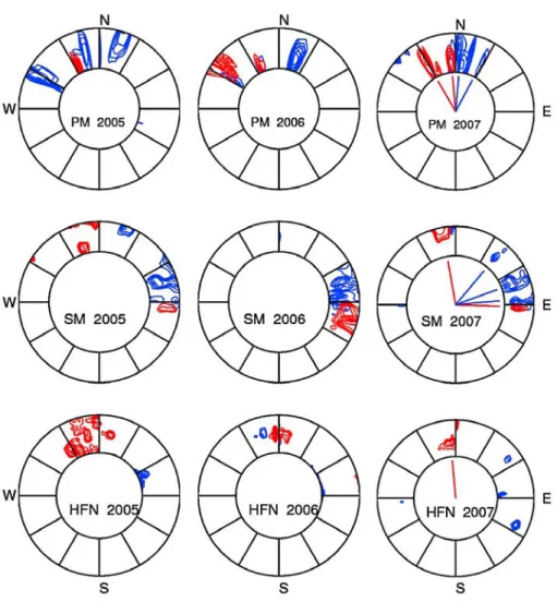
Figure 5. Direction of the microseism sources for station DRV in 2005, 2006, and 2007. For each diagram, the angle is the station back azimuth (azimuth of the source recorded at the station), and the radius corresponds to the frequency band: (top) 0.083 – 0.04 Hz for the primary microseisms, (middle) 0.1 – 0.166 Hz for the long-period secondary microseisms, and (bottom) 0.33 – 0.1667 Hz for the high-frequency secondary microseisms. Contours correspond to the maximum number of polarized signals per month for months January and February in red (local summer) and July and August in blue (local winter). Most abundant directions are plotted as bars for the year 2007.

computed the polarization of seismic noise for three years of data. Figure 5 shows the largest occurrence of polarized signals as a function of azimuth for three period bands: 12– 25 s corresponding to the primary microseisms, 3 – 6 s and 6 – 10 s corre-sponding to the secondary microseism short periods and long periods. The maximum occurrence of polarized signals is normalized to 1 for each month and period band. Contours above 80% of the total amount of polarized signals as a function of period and azimuth are plotted in red for January– February (local summer) and in blue for July –August (local winter). We observe that the source azimuths are not the same for the three period bands, suggesting different source areas. We also see that most of the azimuth variations between winter and summer are repeated every year. The most abundant source azimuths for 2007 are plotted as solid lines at the center of each polar plot and on a map at the station location (Figure 6). Figure 6 shows that all source azimuths are toward the ocean, confirming their oceanic origin. We have also plotted in Figure 6 the sea ice cover in winter (blue) and in summer (red) [Fetterer and Knowles, 2008]. In summer, the island on which the station is installed is surrounded by free water and pieces of ice, and in winter the nearest free sea is about 500 km away.

[25] For the secondary microseism, we observe two

source directions during summer. The direction toward N10W is visible for the entire secondary

microseism period band 3 – 10 s. The source direc-tion N90E only exists for long-period secondary microseisms (6 – 10 s). Bromirski et al. [2005] suggested, considering the H2O ocean bottom station, that local sources may explain short-period secondary microseisms, whereas long-period sec-ondary microseisms may be generated further from the station. Similarly, we suggest that the source along N10W is local whereas the source toward N90E, only observed at long period, is more distant. Indeed, in summer the free ocean is closer toward the North than toward the East where a large area of sea ice is present during the entire summer.

[26] In summer, as the ocean reaches the Dumont

Durville island and Antarctic coast, generation of secondary microseisms by the interaction between incident and coastal reflected ocean waves becomes possible. We speculate that the presence of sea ice in winter inhibits the swell reflection along the coast, leading to fewer secondary microseisms generated by sources that are further away. This is consistent with the low secondary microseism spectral ampli-tudes in winter.

[27] The primary microseism is expected to be

generated at the sloped coast through conversion of ocean waves into Rayleigh waves. We note that the primary microseism source azimuth is always toward the closest free ocean. It seems that in summer the shape of the coast and the presence of many small islands in the vicinity of the station control the dominant source azimuth (N-N20W). In winter, the swell cannot reach the sloped coast due to the presence of sea ice floe, which decreases the generation of primary microseisms and explains the low primary microseism spectral amplitudes. The number of days per year of low primary microseism amplitude is shown in Figure 3. [28] We do not have sufficiently long records yet to

draw conclusions on the impact of global warming on seismic noise, but in the coming years we shall be able to use seismic noise as an independent measure to quantify climate changes.

6. Conclusions

[29] Analysis of seismic noise spectra from the

GEOSCOPE global network has enabled us to show that the secondary microseism amplitude variations are global and depend predominantly on the station latitude and season. Maximum amplitudes are ob-served during local autumn and winter for stations at high latitudes. The seasonal dependence of noise

Figure 6. Geographical map showing DRV station location (gray triangle), Antarctic continent (white), and bathymetry (gray). Sea ice contours [Fetterer and Knowles, 2008] are plotted for the year 2007 in red during local summer and in blue for local winter. Azimuths of the most abundant sources of primary (PM) and secondary (SM) microseisms during local winter (green and blue) and summer (yellow and red) at the station location.

Geochemistry Geophysics Geosystems

G

3

spectra for continental stations in the northern and Southern Hemispheres has been observed by other studies [e.g., Stutzmann et al., 2000; Aster et al., 2008], but here we further show that these seasonal variations are observed for stations at high latitudes and that stations close to the equator have constant noise amplitude.

[30] The good global correlation between

varia-tions of the microseism amplitudes and changes of the highest wave areas suggest that sources of the secondary microseisms are related to these highest wave areas. Analysis of the polarization of the

secondary microseisms shows that, for Northern Hemisphere and equatorial stations, part of (or all) the sources are systematically further south during Northern Hemisphere summer than during winter. These observations show that secondary micro-seism sources generated by ocean waves from the Southern Hemisphere highest wave areas can be recorded by Northern Hemisphere stations when local sources are weak, that is during local summer. For Southern Hemisphere stations, we do not observe significant source direction variations over the year. We speculate that the nearby high ocean

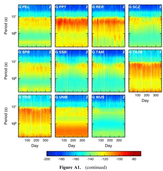
Figure A1. Zoomed in versions of noise diagrams associated with each station presented in Figure 1. Seismic noise amplitude variations over 1 year are plotted in dB with respect to acceleration with the same color scale as in Figure 1.

waves generate most or all of the secondary micro-seisms recorded by these stations. Finally, at the peculiar station DRV close to Antarctica, primary and secondary noise amplitudes are strongly af-fected by changes of the sea ice floe close to the station, and sources of the two microseisms are in different areas.

[31] Thus the analysis of seismic noise spectra and

polarization enables us to track secondary micro-seism source variations, which are closely related to climate variations. Such seismic noise analysis over long periods of time can be used as a new tool to monitor global climate changes.

Appendix A

[32] Figure A1 displays a zoom on the noise

diagrams associated with each station presented in Figure 1. Seismic noise amplitude variations over one year are plotted in dB with respect to acceleration with the same color scale as in Figure 1.

Acknowledgments

[33] This is IPGP contribution 2556. M.S. acknowledges IPGP and the consolider-ingenio 2010 program CSD 2006-00041. The authors thank GEOSCOPE for making data available. Computations were done using the EGEE data grid facilities, and the authors thank David Weissenbach for his help.

References

Aster, R., D. McNamara, and P. Bromirski (2008), Multi-decadal climate-induced variability in microseisms, Seismol. Res. Lett., 79(2), 194 – 202, doi:10.1785/gssrl.79.2.194. Bromirski, P. D., and F. K. Duennebier (2002), The near-coastal

microseism spectrum: Spatial and temporal wave climate relationships, J. Geophys. Res., 107(B8), 2166, doi:10.1029/ 2001JB000265.

Bromirski, P. D., R. E. Flick, and N. Graham (1999), Ocean wave height determined from inland seismometer data: Im-plications for investigating wave climate changes in the NE Pacific, J. Geophys. Res., 104(C9), 20,753 – 20,766, doi:10. 1029/1999JC900156.

Bromirski, P. D., F. K. Duennebier, and R. A. Stephen (2005), Mid-ocean microseisms, Geochem. Geophys. Geosyst., 6, Q04009, doi:10.1029/2004GC000768.

Figure A1. (continued)

Geochemistry Geophysics Geosystems

G

3

estimation of power spectra, coherence and transfer func-tions, J. Geophys. Res., 92, 633 – 648, doi:10.1029/ JB092iB01p00633.

Chevrot, S., M. Sylvander, S. Benahmed, C. Ponsollesand, J. Lefevre, and D. Paradis (2007), Source locations of sec-ondary microseisms in western Europe: Evidence for both coastal and pelagic sources, J. Geophys. Res., 112, B11301, doi:10.1029/2007JB005059.

Fetterer, F., and K. Knowles (2008), Sea ice index, http://nsidc. org/data/seaice_index/, Natl. Snow and Ice Data Cent., Boulder, Colo.

Friedrich, A., F. Kruger, and K. Klinge (1998), Ocean-generated microseismic noise located with the Graffenberg array, J. Seismol., 2, 47 – 64, doi:10.1023/A:1009788904007. Gerstoft, P., and T. Tanimoto (2007), A year of microseisms

in southern California, Geophys. Res. Lett., 34, L20304, doi:10.1029/2007GL031091.

Hasselmann, K. (1963), A statistical analysis of the generation of microseisms, Rev. Geophys., 1, 177 – 209, doi:10.1029/ RG001i002p00177.

Haubrich, R. A., and K. McCamy (1969), Microseisms: Coastal and Pelagic Sources, Rev. Geophys., 7(3), 539 – 571. Kedar, S., M. Longuet-Higgins, F. Webb, N. Graham, R. Clayton,

and C. Jones (2007), The origin of deep ocean microseisms in the North Atlantic Ocean, Proc. R. Soc. A, 464, 777 – 793, doi:10.1098/rspa.2007.0277.

Longuet-Higgins, M. (1950), A theory of the origin of micro-seisms, Philos. Trans. R. Soc., 243, 1 – 35, doi:10.1098/ rsta.1950.0012.

Rascle, N., F. Adrhuin, P. Queffeulou, and D. Croise-Fillon (2008), A global wave parameter database for geophysical

parameters for the open ocean based on traditional parame-terization, Ocean Modell., 25, 154 – 171.

Schimmel, M., and J. Gallart (2003), The use of instantaneous polarization attributes for seismic signal detection and image enhancement, Geophys. J. Int., 155, 653 – 668, doi:10.1046/ j.1365-246X.2003.02077.x.

Schimmel, M., and J. Gallart (2004), Degree of polarization filter for frequency-dependent signal enhancement through noise suppression, Bull. Seismol. Soc. Am., 94, 1016 – 1035, doi:10.1785/0120030178.

Stehly, L., M. Campillo, and N. Shapiro (2006), A study of the seismic noise from its long-range correlation properties, J. Geophys. Res., 111, B10306, doi:10.1029/2005JB004237. Stutzmann, E., G. Roult, and L. Astiz (2000), Geoscope station noise level, Bull. Seismol. Soc. Am., 90, 690 – 701, doi:10. 1785/0119990025.

Stutzmann, E., et al. (2001), MOISE: A prototype multi-parameter ocean bottom station, Bull. Seismol. Soc. Am., 91(4), 885 – 892, doi:10.1785/0120000035.

Tanimoto, T., and L. Riveira (2005), Prograde Rayleigh particle motion, Geophys. J. Int., 162, 399 – 405, doi:10.1111/j.1365-246X.2005.02481.x.

Tanimoto, T., S. Ishimari, and C. Alvizuri (2006), Seasonality in particle motion of microseisms, Geophys. J. Int., 166, 253 – 266, doi:10.1111/j.1365-246X.2006.02931.x.

Webb, S. (1998), Broadband seismology and noise under the ocean, Rev. Geophys., 36(1), 105 – 142, doi:10.1029/ 97RG02287.