HAL Id: hal-00317184
https://hal.archives-ouvertes.fr/hal-00317184
Submitted on 1 Jan 2003
HAL is a multi-disciplinary open access
archive for the deposit and dissemination of
sci-entific research documents, whether they are
pub-lished or not. The documents may come from
teaching and research institutions in France or
abroad, or from public or private research centers.
L’archive ouverte pluridisciplinaire HAL, est
destinée au dépôt et à la diffusion de documents
scientifiques de niveau recherche, publiés ou non,
émanant des établissements d’enseignement et de
recherche français ou étrangers, des laboratoires
publics ou privés.
The local-time variation of the quiet plasmasphere:
geosynchronous observations and kinetic theory
M. A. Reynolds, G. Ganguli, Y.-J. Su, M. F. Thomsen
To cite this version:
M. A. Reynolds, G. Ganguli, Y.-J. Su, M. F. Thomsen. The local-time variation of the quiet
plasmas-phere: geosynchronous observations and kinetic theory. Annales Geophysicae, European Geosciences
Union, 2003, 21 (11), pp.2147-2154. �hal-00317184�
Annales
Geophysicae
The local-time variation of the quiet plasmasphere: geosynchronous
observations and kinetic theory
M. A. Reynolds1, G. Ganguli2, Y.-J. Su3, and M. F. Thomsen4
1Department of Physical Sciences, Embry-Riddle University, 600 S. Clyde Morris Blvd., Daytona Beach, FL 32114, USA 2Beam Physics Branch, Plasma Physics Division, Naval Research Laboratory, 4555 Overlook Avenue SW, Washington, DC
20375, USA
3Laboratory for Atmospheric and Space Physics, University of Colorado, 1234 Innovation Drive, Boulder, CO 80303, USA 4Space and Atmospheric Sciences Group, NIS-1, MS-D466, Los Alamos National Laboratory, Los Alamos, NM 87545, USA
Received: 5 February 2003 – Revised: 31 March 2003 – Accepted: 17 April 2003
Abstract. The quiet-time structure of the plasmaspheric
den-sity was investigated using observations of the Los Alamos geosynchronous satellites, and these observations were com-pared with theoretical predictions of the quasi-static local-time variation by a kinetic model. It was found that the coupling to the ionosphere (via the local-time variation of the exobase) played a key role in determining the density structure at 6.6 RE. The kinetic model predicts that most
of the local-time variation at geosynchronous orbit is due to the variation of the exobase parameters. During quiet times, when the convection electric field is dominated by the coro-tation field, the effects due to flux-tube convection are less prominent than those due to the exobase variation. In ad-dition, the kinetic model predicts that the geosynchronous plasmaspheric density level is at most only 25% of satura-tion density, even when geomagnetic activity is low. The low night-time densities of the ionospheric footpoints, and the subsequent long trapping time scales, prevent the equatorial densities from reaching saturation.
Key words. Magnetospheric physics (magnetosphere-ionosphere interactions; plasma convection; plasmasphere)
1 Introduction
The physical study of the Earth’s plasmasphere has un-dergone a renaissance in the past decade. Evidence of this increased interest can be found in the monograph by Lemaire and Gringauz (1998), the review article by Ganguli et al. (2000), and the special issue of the Journal of Atmo-spheric and Solar-Terrestrial Physics dedicated to D. Carpen-ter (Lemaire and Storey, 2001). Early studies in the 1960s (e.g. Gringauz et al., 1960 and Carpenter, 1966) were able to determine the basic observational facts about the global structure of the plasmasphere and plasmapause, and to de-duce the basic physics of magnetospheric convection that
Correspondence to: M. A. Reynolds
was taking place (Axford and Hines, 1961). Detailed dynam-ical studies were performed in the 1970s (e.g. Grebowsky, 1970) and much of the inner magnetosphere was thought to be understood. The space physics community then turned the bulk of their attention to other areas in the 1980s: for exam-ple, the magnetopause, tail dynamics, storms and substorms, and auroral phenomena. However, there remained two fun-damental processes in which the physical mechanisms had yet to be definitively determined: the refilling of plasmas-pheric flux tubes after being depleted, and the formation of the plasmapause boundary. The first of these is an aspect of magnetosphere-ionosphere coupling, while the second is a consequence of the solar wind-magnetosphere interaction and the resulting convection driven by the large-scale elec-tric field. Evidence of the importance of these two funda-mental processes can be found in papers concerning the cou-pling with the ionosphere (Singh and Horwitz, 1992) and the physics of plasmapause formation (Lemaire, 1974). The spa-tial structure of the quiet plasmasphere, an issue related to the first process (refilling), is the focus of this paper.
One of the underlying properties of the plasmasphere, the density structure during steady convection and low geomag-netic activity, is not well known. There are two reasons for this: it is not often continuously quiet for very long, and, as with other space studies, the satellite coverage is poor (though the IMAGE and Cluster missions are beginning to al-leviate the second problem). Here, we investigate this quiet-time structure using the observations from the Los Alamos National Laboratory (LANL) geosynchronous satellites, as well as a kinetic model. First, we identify long (≥ 2 days) pe-riods of low magnetic disturbance. This implies that the con-vection electric field is weak, that the plasmasphere extends out beyond 6.6 RE in the equatorial plane, and the
geosyn-chronous flux tubes have had a good chance to at least par-tially refill. Second, we look at the entire Los Alamos data set (1990–2000) during these quiet periods, and evaluate the plasma density as a function of local time. Finally, we com-pare these observations with our kinetic model that includes ionospheric coupling via exobase parameters that vary with
2148 M. A. Reynolds et al.: The local-time variation of the quiet plasmasphere local time.
There have been several recent studies of plasmaspheric refilling using observations of the LANL satellites at geosyn-chronous orbit (Thomsen et al., 1998; Lawrence et al., 1999; Su et al., 2001). This series of three papers character-izes the temporal variation of the plasma density at geosyn-chronous orbit that is indicative of the refilling process. One of their main conclusions was that refilling occurs in a two-stage process. During the first 24 hours of a quiet period (called “early time”), the rate of increase of the density is small (<5 cm−3day−1), while after the first day (called “late time”) the rate of increase is larger (≈10–25 cm−3day−1). The first 24 hours is also characterized by a low plasma den-sity (n < 10 cm−3), indicating that the geosynchronous flux
tubes had recently been emptied (this condition is usually considered to be the plasma trough). In the studies of late-time refilling, however, the refilling rate was obtained from the density measurements taken at a single local time on con-secutive days, and the detailed structure of the local time variation was not investigated. Here, we focus specifically on the local time variation with the understanding that this variation is superimposed on a secularly increasing density due to refilling. This late time is characterized by a larger plasma density (n > 10 cm−3), and is usually considered to be plasmasphere proper.
The kinetic model that we use here, the Multi-Species Ki-netic Plasmasphere Model (MSKPM) (Reynolds et al., 1999, 2001), is collisionless, so that neither Coulomb collisions nor wave-particle effects are included directly. The most impor-tant factors that determine the geosynchronous density are the conditions at the exobase (i.e. the footpoint of the field line) and the density of particles that have been trapped (i.e. scattered from the loss cone into the trapped region of veloc-ity space).
Including trapped particles effectively includes Coulomb collisions in an ad hoc manner. Using a parameterization of the FLIP (Field Line Interhemispheric Plasmasphere) (e.g. Richards and Torr, 1986) model to represent the conditions at the exobase and varying the fraction of trapped parti-cles, MSKPM is able to reproduce the diurnal variation of the geosynchronous density measurements well. From this agreement, the maximum refilling percentage is found to be on the order of 25%. Geomagnetic conditions are probably never quiet long enough for the geosynchronous plasmas-pheric density to completely saturate.
In Sect. 2 the criterion used to filter out the geomagnet-ically quiet periods in the past decade is explained; Sect. 3 describes the observations of refilling at geosynchronous or-bit; Sect. 4 shows the LANL plasma density observations; and Sect. 5 compares the predictions of MSKPM with the statistical observations.
2 Quiet-time criterion
For the purposes of this study we use the magnetic activity in-dex Kpas a proxy for determining whether the plasmasphere
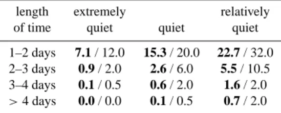
Table 1. Yearly occurrence frequency of different lengths of quiet periods. Bold numbers are for the entire Kpdatabase (1932–2000)
and non-bold refer to the two-year period during solar minumum (1996–1997)
length extremely relatively of time quiet quiet quiet 1–2 days 7.1 / 12.0 15.3 / 20.0 22.7 / 32.0 2–3 days 0.9 / 2.0 2.6 / 6.0 5.5 / 10.5 3–4 days 0.1 / 0.5 0.6 / 2.0 1.6 / 2.0
>4 days 0.0 / 0.0 0.1 / 0.5 0.7 / 2.0
is in a quiet state or a disturbed state. One of the reasons for this choice is that there is an established correlation between the solar wind as a driver and the magnetospheric response as measured by Kp(e.g. Crooker et al., 1977). Another reason
is that there has been significant work on the refilling of the geosynchronous plasmasphere using Kp as a proxy (see the
work cited below in Sect. 3), and we build on this previous work.
In order for it to be likely that L = 6.6 is within the plas-masphere (i.e. in the refilling process), we focus on time periods when Kpis low. We call these steady periods quiet
and we define three levels of quiet “relatively quiet” : Kp≤1+
“quiet” : Kp≤1
“extremely quiet” : Kp≤1−.
Which of these is the most suitable criterion for the present study can be determined from a study of Table 1, which lists the yearly occurrence frequencies of various lengths of quiet periods for the entire 69-year history of recorded Kp values
(January 1932–December 2000). Of course, such quiet peri-ods are more likely to occur during solar minimum, and the yearly occurence frequencies during the quiet years 1996– 1997 are also shown in Table 1. It can be seen that long periods that are “extremely quiet” do not occur frequently enough to be statistically useful in the 10 years of satellite data available. Lawrence et al. (1999) chose the “relatively quiet” criterion to measure late-time refilling, but we wish to look at less disturbed periods so that it is more likely that L =6.6 is truly within the plasmasphere. Hence, we choose the “quiet” criterion as our benchmark. In addition, since it takes several days for the plasmasphere to fill at the equator of an L = 6.6 field line, only those periods that are quiet for longer than two days are considered. A list of such periods in the years 1990–2000 is shown in Table 2.
Periods longer than two days that are less disturbed than “extremely quiet” happen rarely. For example, the more stringent condition (Kp ≤ 0+) occurs only about once
ev-ery five years, and it happened only twice during the 1990s. Periods longer than two days that are more disturbed than “relatively quiet” happen quite often. For example, the less stringent condition (Kp ≤ 2−) occurs approximately 14
Fig. 1. Density measured by satellite 1994-084 for six days in De-cember 1997, and Kp for the same time period. This particular
satellite passed through local noon at approximately 05:00 UT each day, and these times are marked with the vertical dashed lines.
is useful statistically, there is a smaller probability that the satellites are within the plasmasphere (due to the increased strength of the convection electric field), and it is more diffi-cult to argue that this level of activity constitutes quiet. The longest “quiet” period in the 1990s lasted 5.6 days on 24–29 December 1997. Except for this one instance, however, the longest “quiet” period in the 11 years under study was 3.3 days. The length of these periods along with the measured re-filling rate suggest that the plasmasphere at geosynchronous orbit is rarely, if ever, fully saturated.
3 The refilling process at geosynchronous orbit
There has been considerable work on the refilling process, both on the physical mechanisms involved, as well as the ob-servations (Singh and Horwitz, 1992). Most obob-servations, however, have been made by satellites that did not remain co-located with a particular flux tube, making it difficult to evaluate the past history in order to measure the refilling rate. The Los Alamos geosynchronous satellites are uniquely situ-ated to provide this type of observation, although the plasma-sphere does not often extend to L = 6.6, except during times of prolonged quiet. In addition, these satellites have been op-erational since 1990, resulting in a large database that spans a solar cycle.
Thomsen et al. (1998) looked in detail at observations of early-time refilling as measured by the magnetospheric plasma analyzers on the Los Alamos geosynchronous satel-lites. (They analysed several months in 1990, 1991, and 1996.) Specifically, they looked at the occurrence frequency distributions of the cold ion density in one-hour local-time bins, and were able to calculate a refilling rate of about 1.5 cm−3day−1. This result was restricted to the dayside (6– 15 MLT) and took the 25th percentile level as the best mea-sure of the trough density (this percentile level was steady and relatively uncontaminated by encounters with the dense
Table 2. The set of 31 periods that were “quiet” for at least two days during the study 1990–2000
Start
Year Month Day Length 1990 Nov 04 3.3 Nov 13 2.4 1993 May 24 2.5 1995 Mar 20 2.5 Jun 11 3.0 Jul 04 2.1 Jul 09 2.8 Nov 23 2.5 1996 Apr 06 2.1 Jun 12 2.8 Jul 09 2.4 Nov 01 2.6 Dec 05 2.3 Dec 18 2.3 1997 Jan 15 2.1 Mar 08 2.1 May 11 3.0 Jun 12 2.4 Jul 12 3.1 Aug 25 2.0 Oct 04 2.0 Nov 27 3.1 Dec 07 2.5 Dec 12 3.5 Dec 24 5.6 1998 Feb 05 2.9 Feb 15 2.1 1999 Jan 31 2.8 Jun 20 2.3 Dec 21 2.6 2000 Mar 15 2.0
plasmasphere). This value agreed with previous studies, as well as the model of Carpenter and Anderson (1992).
A more comprehensive study was performed by Lawrence et al. (1999), who confirmed the early-time refilling rate, but also investigated the late-time refilling characteristics. Ex-tending the time period to 4 consecutive years (1993–1997), they measured the density over the course of several days, but they looked at the same local time each day of the refilling (e.g. 11:00–13:00 LT), which captures the secular increase in density, but not the local time variation on time scales less than one day. (They defined a refilling event as a period of Kp ≤1+, i.e. “relatively quiet,” for at least 1.5 consecutive
days, as well as requiring that at least one satellite observed significant plasma density. The fact that not all satellites ob-served refilling events simultaneously can be understood in the light of recent observations of the EUV instrument on the IMAGE satellite (Burch, 2001), where the outer plasma-sphere is highly structured and is composed of fingers and shoulders. (This feature has, of course, been known since
2150 M. A. Reynolds et al.: The local-time variation of the quiet plasmasphere
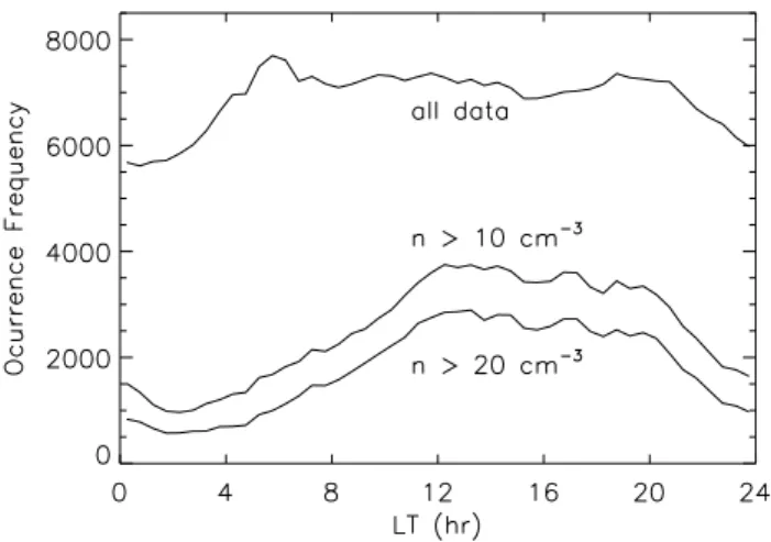
Fig. 2. Occurrence frequency (per half hour bin) of density mea-surements as a function of local time. The thick line includes all measurements of the 117 satellite data sets, while the thin lines ex-clude the low-density measurements.
the early LANL geosynchronous satellites: Moldwin et al., 1995). Depending on the local time, the measured refill-ing rate was 10–25 cm−3day−1, which is significantly larger
than the early-time rate. This evidence was key to the de-scription of a two-stage refilling process: during the first day the density is low (less than 10 cm−3) and the refilling rate is also low, while after the first day, the density typically climbs to larger than 10 cm−3 and the refilling rate is correspond-ingly larger and is due primarily to Coulomb collisions.
Both of the above studies, however, assumed that the flux tubes were exactly corotating with the spacecraft. As an im-provement, Su et al. (2001) reevaluated the early time results of Thomsen et al. (1998) and Lawrence et al. (1999) by uti-lizing a realistic convection electric field, which can modify the assumed refilling time by up to 2 h, as well as using a ten-year period (1990–2000). With this more sophisticated model, the early-time refilling rate was slightly modified to 2.5–6.5 cm−3day−1. The late-time refilling rate was evalu-ated in the same way as Lawrence et al. (1999), using the larger database, and the observed rate was identical. With late-time refilling, no assumptions about the convection pat-tern were made, since only the local time was used to de-termine the rate. Thus, Su et al. (2001) came to the same conclusions regarding the two stage nature of the refilling process.
The local time variation of the density can be seen in some of the figures from these previous studies. For exam-ple, Figs. 4 and 6 of Lawrence et al. (1999) show that the early-time density decreases after ∼16:00 LT, and the late-time density fluctuates over the course of 24 h, respectively. Here, we focus on this diurnal variation during the late time refilling process.
4 Geosynchronous observations
Figure 1 shows the density measured by satellite 1994-084 during 24–29 December 1997. For comparison, the magnetic index Kp is also shown. There had been a minor storm on
10–11 December, where Dstreached −50 nT. Another minor
storm occurred on 30 December. Between the two storms, however, magnetic activity was low, with Kpreaching 2 only
a few times. At geosynchronous orbit during this interval, the density was large on the dayside (∼100 cm−3) and smaller on the nightside (∼20 cm−3), with several “drainage” events occurring resulting in empty flux tubes. Figure 1 depicts one of these drainage events and the subsequent refilling of the flux tubes. The clear diurnal variation superimposed on top of the secular increase is what we wish to characterize. Not all of the quiet-time satellite measurements show a refilling as clearly as that in Fig. 1, but almost all show a similar lo-cal time variation. Those that do not show such a variation typically measure densities less than 10 cm−3and hence, are
probably not in the plasmasphere proper. In order to exclude such measurements, we do not include any density measure-ment smaller than 10 cm−3. Section 4.2 discusses the details of this choice.
There are 117 satellite data sets over the 31 selected pe-riods, as anywhere from three to five LANL satellites were taking data during each period. As mentioned above, the oc-currence frequency is expected to be larger during solar min-imum, and this is confirmed by the fact that 17 out of the 31 periods took place in the two years 1996 and 1997.
4.1 Observational statistics
In order to assess the quality of the measurements, a detailed look at the statistics is in order. The density measurements of all 117 satellite data sets were grouped into 48 bins (of width 30 min) in local time. Figure 2 shows the number of mea-surements (or occurrence frequency) in each bin. There are 358 097 measurements in total, with approximately 7 400 in each half-hour bin, and fairly even coverage over the entire day. Most of these measurements, however, were of low-density plasma (n < 10 cm−3), and Fig. 2 also shows the number of measurements in each bin that had values greater than 10 cm−3and greater than 20 cm−3. The occurrence fre-quencies of the high-density measurements in local-time are not so even. The reason for this can be seen from a compari-son with Fig. 1. During the refilling process, even though the densities in the afternoon sector may reach values of 20 cm−3 or more, the nighttime densities often fall below this value. Therefore, higher densities are more commonly encountered in the afternoon, and this is reflected in the occurrence fre-quency. (This result is well known, and has been observed by the Los Alamos satellites since their launch.)
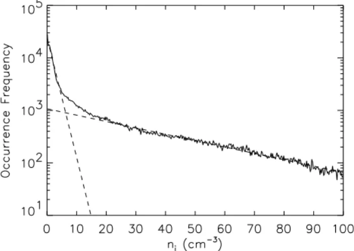
Because most of the measurements are of low-density plasmas, it is illustrative to investigate the occurrence fre-quency as a function of density, shown in Fig. 3, where bins of width 0.25 cm−3 are used. It is clear that for densities larger than 20 cm−3 (corresponding to late-time refilling),
Fig. 3. Occurrence frequency of density measurements summed over local time as a function of density. All half-hour bins show a similar behavior. The bin width here is 0.25 cm−3. The dotted lines are the best linear fits to the data for n < 5 cm−3and n > 20 cm−3.
there is no definite peak that indicates a most probable value for the density. This is in contrast to the densities smaller than 5 cm−3 (corresponding to early-time refilling), where a slight peak can be seen. This peak is even clearer when higher resolution in density is used and a single local time is selected (Thomsen et al., 1998). In fact, this definite peak in occurrence frequency was near 1–2 cm−3, which was ap-proximately coincident with the 25th percentile (see Fig. 10 of Thomsen et al., 1998). This was an additional reason to conclude that the 25th percentile represented the best mea-sure of the trough density.
Even though there is no peak in Fig. 3, there is a change in slope near 10 cm−3, indicating that the character of the measurements is different for large densities than for small densities. Also shown in Fig. 3 are the best linear fits to the occurrence frequency for densities restricted to n < 5 cm−3 (definitely early time) and n > 20 cm−3 (definitely late time). Since these densities are representative of early and late-time refilling, the demarcation between the two den-sity regions must be between 5 and 20 cm−3. The actual
choice is somewhat arbitrary, however, because the change in slope is gradual. Because Fig. 2 shows that the local time characteristics do not change dramatically between 10 cm−3 and 20 cm−3, and because 10 cm−3 has historically been the lower density limit for the plasmasphere at at geosyn-chronous orbit, we restrict our analysis to those densities larger than 10 cm−3. A more statistically accurate demarca-tion can perhaps be determined, but the results of this study would not be strongly affected.
4.2 Density measurements
In addition, our interest in the high density, late-time refill-ing plasmasphere leads us to choose the 75th percentile as our best measure of the appropriate density. Similar to the early-time criterion, we expect that the 75th percentile level
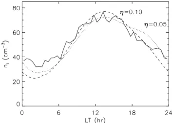
Fig. 4. The solid curves are the 25th, 50th and 75th percentile densi-ties, and the dashed curve is the best fit cosine to the 75th percentile, given by n(cm−3) =53.2 + 18.0 cos(LT − 13.4 h).
is relatively uncontaminated by encounters with low density plasma. The exact value of this choice is not critical, as all percentile levels exhibit similar local-time behavior. In fact, Su et al. (2001), who chose the 70th percentile, showed that the choice of percentile level affects the numerical value of the density, but does not affect the trend of refilling. That is, they found similar late-time refilling rates regardless of the percentile chosen. This can be seen in Fig. 4, which shows the 25th, 50th, and 75th percentile levels (after removing all measurements less than 10 cm−3). All three show a similar variation as a function of local time.
Three observations can be made about Fig. 4. First, the 75th percentile is closely represented by a sinusoidal vari-ation, shown for comparison. It is a cosine with a maxi-mum near 13.4 h. This phase lag can also be seen clearly in Fig. 1. Second, this variation is similar to the density of the ionosphere at 2000 km, as given by the International Ref-erence Ionosphere. Third, this variation is nearly identical with the trough density model recently proposed by Sheeley et al. (2001) that was deduced from CRRES observations. For L = 6.6, they obtained (their Eq. 7)
n(cm−3) =5.29 + 2.28 cos(LT − 13.6 h). (1) The phase offset from noon is the same as that obtained here, and while the density is much lower, the amplitude of the variation is 40% of the average value, compared with 34% at geosynchronous orbit. The fact that the CRRES satellite samples many different L-shells and the observations were not limited to low Kpsuggests that typical geosynchronous
densities are fairly low (which is what is observed). The higher densities only appear during quiet periods.
5 Kinetic theory
MSKPM was developed to address the collisionless nature of the plasma at high altitudes on closed, dipolar field lines.
2152 M. A. Reynolds et al.: The local-time variation of the quiet plasmasphere
Fig. 5. MSKPM predictions with a uniform exobase and the parametrized FLIP exobase that varies with local time. The FLIP exobase is given by Eqs. 3–5, and the uniform exobase is obtained by using only the constant terms in the FLIP exobase.
Starting with the conditions at the exobase (altitude, density, temperature, composition), the velocity distribution func-tions are followed as the particles move along the field lines and also as they convect diurnally. Particles in the loss cone (ballistic and passing), as well as those that are trapped are included, and the convection electric field used is E5D (McIl-wain, 1986). The phase-space density of the trapped particles relative to the phase-space density of those in the loss cone is chosen empirically through the magnitude of a parameter η, where 0 < η < 1. The lower value indicates that there are no trapped particles, and the upper value indicates that the trapped region is full, close to diffusive equilibrium. The loss cone is always full (i.e. for all values of η).
If η is nonzero, then those trapped particles exist due to pitch-angle scattering of particles from the loss cone. This parameterization, therefore, includes the lowest-order ef-fect of Coulomb collisions. More detailed descriptions of MSKPM can be found in Reynolds et al. (1999, 2001).
Convection via the radial excursion of flux tubes strongly affects the density and temperature structure of the outer plasmasphere. The main effect is a density enhancement in the post-midnight sector, where the flux tubes are closest to the Earth (there is also an increase in the parallel tempera-ture and a decrease in the perpendicular temperatempera-ture). This enhancement is shown in Fig. 5, where the dashed lines in-dicate the density at the magnetic equator of the L = 6.6 field line for the case when the exobase conditions are con-stant in local time. The η = 0 case predicts a density that is uniform in local time, since the compression and rarefaction of the convecting flux tubes affect only the trapped particle density. For nonzero values of η, the post-midnight density enhancement is clearly seen.
However, the conditions at the exobase also strongly affect the global structure, and this can overwhelm the effects of convection (Reynolds et al., 2001). Which one dominates
de-Fig. 6. Comparison between observations and model. The solid line is the 75th percentile level, the dotted line is the MSKPM prediction with η = 0.05 reduced by a factor of 2.9, and the dashed line is with
η =0.10 reduced by a factor of 5.5.
pends on the relative strength of the exobase variation in local time compared to the asymmetry of the convection electric field. For the present case of quiet geomagnetic conditions, i.e. when the dawn-dusk electric field is weak, the exobase variation almost completely overwhelms the compression of the flux tubes due to convection.
The original parameterization of the exobase parameters (Reynolds et al., 2001) predicted by FLIP has been gener-alized to include the phase of the exobase variation. This phase shift (away from a strictly noon-midnight asymmetry) can be seen in Fig. 4, where the density measurements have a maximum that is shifted 1.4 hours later than noon. The FLIP calculation also shows this phase shift, and our updated pa-rameterizations are
n0(cm−3) =4280 + 2670 cos(LT − 13.6 h), (2)
h0(km) = 3590 + 1960 cos(LT − 23.6 h), (3)
nH e/n0=0.0297 + 0.0185 cos(LT − 12.7 h), (4)
T0(K) = 2510 + 1300 cos(LT − 13.4 h), (5)
where h0, n0, nH e and T0 are the exobase altitude, total
density, helium density, and temperature, and LT is the lo-cal time. With these exobase conditions, the predictions of MSKPM for four values of η are shown in Fig. 5. Clearly, the post-midnight density enhancement due to convection is overwhelmed by the diurnal variation of the exobase. Also clearly, the density variation predicted when η = 0.15 is much stronger than the measured variation, and that pre-dicted when η = 0 has the wrong phase. This implies that the average value of η during the late-time refilling phase is on the order of 0.05–0.10, which means that, while the flux tube’s density varies diurnally, on average, it is approx-imately 10% of saturation (the loss cone angle at geosyn-chronous orbit, for scattering at 3590 km, is approximately 4.9◦, so the volume of velocity space occupied by the
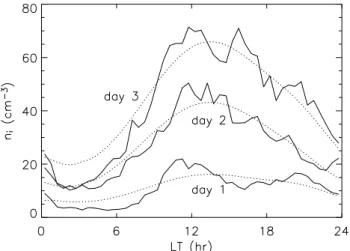
parti-Fig. 7. Observations of the 75th percentile level during the first day, second day, and third day of a quiet period (solid lines). The dotted lines are the best fit MSKPM predictions. For day 1, η = 0.05 reduced by a factor of 13.1. For day 2, η = 0.12 reduced by a factor of 11.8. For day 3, η = 0.08 reduced by a factor of 5.1.
cles in the loss cone is 0.37% of the total volume, which is negligible).
The predicted densities assuming η = 0.05 and η = 0.10 are compared with the 75th percentile level of the geosyn-chronous measurements in Fig. 6. Of course, the predicted densities are larger than the 75th percentile, but the local-time variation is almost identical. In order to show them on the same scale, the MSKPM predictions are reduced by fac-tors of 2.9 (η = 0.05) and 5.5 (η = 0.10). This simply means, for example, that the absolute values of the densities in Eq. (2) are not correct, but that the phase shift and the rel-ative size of the variation are correct. There are other ways to reduce the density at L = 6.6 than by reducing the exobase density, but the effects of Eqs. (3)–(5) are more nonlinear and not so easily evaluated.
A more useful comparison can be made by realizing that the amplitude of the variation, and hence, the velocity-space anisotropy, changes as a function of time. As can be seen in Fig. 1, there is a secular increase in density along with a diurnal variation. These observations imply that the density has not yet reached a saturated state by the third quiet day be-cause the secular increase is still ocurring. To investigate the secular behavior, we separate out the density measurements taken during the first day of each quiet period (i.e. early-time refilling) from those taken on the second day as well as those taken on the third day. Table 2 shows that very few quiet pe-riods last longer than three days, while looking at later times does not prove statistically meaningful.
Figure 7 shows the 75th percentile of the density measure-ments on these three days (collected in bins of 30 min, as before). Here, however, we do not restrict the density to be greater than 10 cm−3, because this density is rarely observed on the first day (and is also rare in the post-midnight sector on later days – which suggests that this local time sector has saturated by the second day of quiet). For most times,
how-ever, the density continues to increase through the third quiet day (and probably beyond, although there is not enough data to state this conclusively).
Also shown in Fig. 7 are least-squares best fits of MSKPM predictions using various values of η. Because the amplitude of the observed diurnal density variation increases with time, a comparison with Fig. 5 suggests that the value of η should increase with time. The first day best fit results in the lowest value η = 0.05, but the second day comparison results in a larger value (η = 0.12) than the third day (η = 0.08). The fact that η does not increase monotonically is due to the shape of the observations from the third day: the best fit agrees well in the dusk sector, but not very well post-midnight. A simple modification to the fitting procedure will change this: forcing only the amplitude to match results in a best fit for the third day of η ≈ 0.25. Also, the scatter in the observations (even after binning in local time) makes the comparison nontrivial, but the trend is clear – η increases each day.
On the other hand, pitch-angle anisotropy is rarely ob-served by the LANL satellites, when the cold ion density becomes larger than 10 cm−3. However, there are occasions when field-aligned warm and isotropic cold populations co-exist (Moldwin et al., 1995). These observations do not seem to be consistent with the physical requirement that the newly upflowing plasma from the topside ionosphere each morning should be anisotropic, even after long periods of quiet, when the densities are on the order of 30–40 cm−3. This paradox
deserves further study.
6 Conclusion
This study has been an attempt to determine the underlying local-time structure of the plasmasphere. Because the geo-magnetic activity is not continuously low for extended peri-ods, the outer plasmaspheric density rarely reaches a steady state, and this underlying structure is difficult to determine. In addition, the diurnal variation of a flux tube’s ionospheric footpoint means that, even for low activity, the outer plasma-sphere is in dynamic equilibrium. This dynamic equilibrium consists of the topside ionosphere refilling the loss cone of the plasmaspheric flux tubes during the day and emptying the loss cone at night. Of course, this means that η will, in reality, vary with local time, as well as because the pitch-angle scattering rate between the loss cone and the trapped population will vary. Here, we are able to look at the secular increase of η, and we leave the diurnal variation for future work. Here, our chosen approach to determine the structure is a statistical study, focusing on times when the geomagnetic activity was low for at least two consecutive days.
Two conclusions follow from the measured and predicted local-time structures in Fig. 6. First, the refilling plasmas-phere simply mimics the variation of the underlying iono-sphere. This implies that the coupling between the plasmas-phere and the topside ionosplasmas-phere is strong, and confirms that the ballistic time scale for ionospheric particles to populate the equatorial region is on the order of one hour. However,
2154 M. A. Reynolds et al.: The local-time variation of the quiet plasmasphere the fact that the maximum value of η is on the order of 0.25
implies that the scattering time scale is much longer. Second, the geosynchronous plasmasphere is rarely, if ever, completely saturated and full of plasma. From a ki-netic point of view, the processes that scatter particles from the loss cone occur slowly, and it takes the trapped region several days (Lemaire, 1989) rather than several hours (while the footpoint is in sunlight) to be populated. Of course, on lower L-shells the loss cone is larger, a large density exists at the field line apex due to the presence of ballistic and passing particles, and the time scale for scattering into the trapped region is shorter. This implies that the lower L-shells should exhibit a weaker local-time density variation. This prediction is currently being investigated using both data from the EUV instrument on the IMAGE satellite, as well as ULF resonance techniques.
Acknowledgements. This work is sponsored by the Office of Naval Research, the National Aeronautics and Space Administration, and the Research Fund at Embry-Riddle University. We thank A. Cephas, R. Adams, O. Jones, I. Petrov, and L. Novak for their as-sistance with programming and graphics, and J. Wanliss for useful discussions.
The Kp data was obtained from the World Data Center for
Ge-omagnetism in Copenhagen, Denmark which is run by the Solar-Terrestrial Physics Division of the Danish Meteorological Institute. Topical Editor T. Pulkkinen thanks J. Lemaire and M. Moldwin for their help in evaluating this paper.
References
Axford, W. I., and Hines, C. O.: A unifying theory of high-latitude geophysical phenomena and geomagnetic storms, Can. J. Phys., 39, 1433–1464, 1961.
Burch, J. L., Mende, S. B., Mitchell, D. G., Moore, T. E., Pollock, C. J., Reinisch, B. W., Sandel, B. R., Fuselier, S. A., Gallagher, D. L., Green, J. L., Perez, J. D., and Reiff, P. H.: Views of the earth’s magnetosphere with the IMAGE satellite, Science, 291, 616–624, 2001.
Carpenter, D. L.: Whistler studies of the plasmapause in the magne-tosphere, 1. Temporal variations in the position of the knee and some evidence on plasma motions near the knee, J. Geophys. Res., 71, 693–709, 1966.
Carpenter, D. L and Anderson, R. R.: An ISEE/whistler model of equatorial electron density in the magnetosphere, J. Geophys. Res., 97, 1097–1108, 1992.
Crooker, N. U., Feynman, J., and Gosling, J. T.: On the high corre-lation between long-term averages of solar wind speed and geo-magnetic activity, J. Geophys. Res., 82, 1933–1937, 1977. Ganguli, G., Reynolds, M. A., and Liemohn, M. W.: The
plasma-sphere and advances in plasmaspheric research, J. Atm. Solar-Terr. Phys., 62, 1647–1657, 2000.
Grebowsky, J. M.: Model study of plasmapause motion, J. Geo-phys. Res., 75, 4329–4333, 1970.
Gringauz, K. I., Bezrukikh, V. V., Ozerov, V. D., and Rybchin-sky, R. E.: The study of the interplanetay ionized gas, high en-ergy electrons and corpuscular radiation of the Sun, employing three-electrode charged particle traps on the second Soviet space rocket, Soviet Phys. Doklady, 5, 361–364, 1960.
Lawrence, D. J., Thomsen, M. F., Borovsky, J. E., and McComas, D. F.: Measurements of early and late time plasmasphere refilling as observed from geosynchronous orbit, J. Geophys. Res., 104, 14 691–14 704, 1999.
Lemaire, J. F. and Gringauz, K. I.: The Earth’s Plasmasphere, 350 pp., Cambridge Univ. Press, New York, 1998.
Lemaire, J. and Storey, L. R. O.: The plasmasphere revisited: A tribute to Donald Carpenter, J. Atm. Solar-Terr. Phys., 63, 1105– 1106, 2001.
Lemaire, J.: The “Roche-limit” of ionospheric plasma and the for-mation of the plasmapause, Planet. Space Sci., 22, 757, 1974. Lemaire, J.: Plasma distribution models in a rotating magnetic
dipole and refilling of plasmaspheric flux tubes, Phys. Fluids B, 1, 1519–1525, 1989.
McIlwain, C. E.: A Kp dependent equatorial electric field model,
Adv. Space Res., 6(3), 187–197, 1986.
Moldwin, M. B., Thomsen, M. F., Bame, S. J., and McComas, D.: The fine-scale structure of the outer plasmasphere, J. Geophys. Res., 100, 8021–8029, 1995.
Reynolds, M. A., Ganguli, G., Lemaire, J., Fedder, J. A., Meier, R. R., and Mel´endez-Alvira, D. J.: Thermal plasmaspheric mor-phology: Effect of geomagnetic and solar activity, J. Geophys. Res., 104, 10 285–10 294, 1999.
Reynolds, M. A., Mel´endez-Alvira, D. J., and Ganguli, G.: Equa-torial coupling between the plasmasphere and the topside iono-sphere, J. Atm. Solar-Terr. Phys., 63, 1267–1273, 2001. Richards, P. G. and Torr, D. G.: Thermal coupling of conjugate
ionospheres and the tilt of the Earth’s magnetic field, J. Geophys. Res., 91, 9017–9021, 1986.
Sheeley, B. W., Moldwin, M. B., Rassoul, H. K., and Anderson, R. R.: An empirical plasmasphere and trough density model: CR-RES observations, J. Geophys. Res., 106, 25 631–25 641, 2001. Singh, N. and Horwitz, J. L.: Plasmasphere refilling: Recent
obser-vations and modeling, J. Geophys. Res., 97, 1049, 1992. Su, Y.-J., Thomsen, M. F., Borovsky, J. E., and Lawrence, D. J.:
A comprehensive survey of plasmasphere refilling at geosyn-chronous orbit, J. Geophys. Res., 106, 25 615–25 629, 2001. Thomsen, M. F., McComas, D. J., Borovsky, J. E., and Elphic, R.
C.: The magnetospheric trough, in Geospace Mass and Energy Flows: Results from the International Solar-Terrestrial Physics Program, Geophys. Monogr. Ser., Vol. 104, J. L. Horwitz, D. L. Gallagher, and W. K. Peterson (Eds), Washington, DC, pp. 355– 369, 1998.

![Risiko- & [und] Schutzfaktoren der psychischen Gesundheit humanitärer Einsatzhelfer : eine systematische Literaturübersicht](data:image/gif;base64,R0lGODlhAQABAIAAAP///wAAACH5BAEAAAAALAAAAAABAAEAAAICRAEAOw==)