HAL Id: inria-00331906
https://hal.inria.fr/inria-00331906
Submitted on 20 Oct 2008
HAL is a multi-disciplinary open access archive for the deposit and dissemination of sci-entific research documents, whether they are pub-lished or not. The documents may come from teaching and research institutions in France or abroad, or from public or private research centers.
L’archive ouverte pluridisciplinaire HAL, est destinée au dépôt et à la diffusion de documents scientifiques de niveau recherche, publiés ou non, émanant des établissements d’enseignement et de recherche français ou étrangers, des laboratoires publics ou privés.
Luc Buatois, Guillaume Caumon, Bruno Lévy
To cite this version:
Luc Buatois, Guillaume Caumon, Bruno Lévy. Concurrent number cruncher - A GPU implementation of a general sparse linear solver. International Journal of Parallel, Emergent and Distributed Systems, Taylor & Francis, 2008, 24 (3), pp.205-223. �10.1080/17445760802337010�. �inria-00331906�
Concurrent number cruncher
A GPU implementation of a general sparse linear solver
Luc Buatois1,2∗, Guillaume Caumon1and Bruno Lévy2
1ENSG/CRPG, Gocad Research Group, Nancy University,
Rue du Doyen Roubault
BP40 54501 Vandoeuvre-les-Nancy, France
2INRIA Lorraine, ALICE,
BP 239 - 54506 Vandoeuvre-les-Nancy Cedex, France
Abstract
A wide class of numerical methods needs to solve a linear system, where the matrix pat-tern of non-zero coefficients can be arbitrary. These problems can greatly benefit from highly multithreaded computational power and large memory bandwidth available on GPUs, espe-cially since dedicated general purpose APIs such as CTM (AMD-ATI) and CUDA (NVIDIA) have appeared. CUDA even provides a BLAS implementation, but only for dense matrices (CuBLAS). Other existing linear solvers for the GPU are also limited by their internal matrix representation.
This paper describes how to combine recent GPU programming techniques and new GPU dedicated APIs with high performance computing strategies (namely block compressed row storage, register blocking and vectorization), to implement a sparse general-purpose linear solver. Our implementation of the Jacobi-preconditioned Conjugate Gradient algorithm out-performs by up to a factor of 6.0x leading-edge CPU counterparts, making it attractive for applications which content with single precision.
Keywords: graphics processors, parallel processing, sparse numerical solver
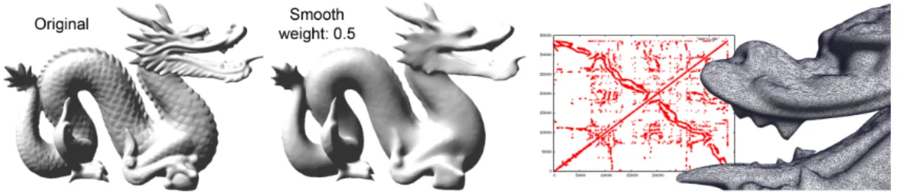
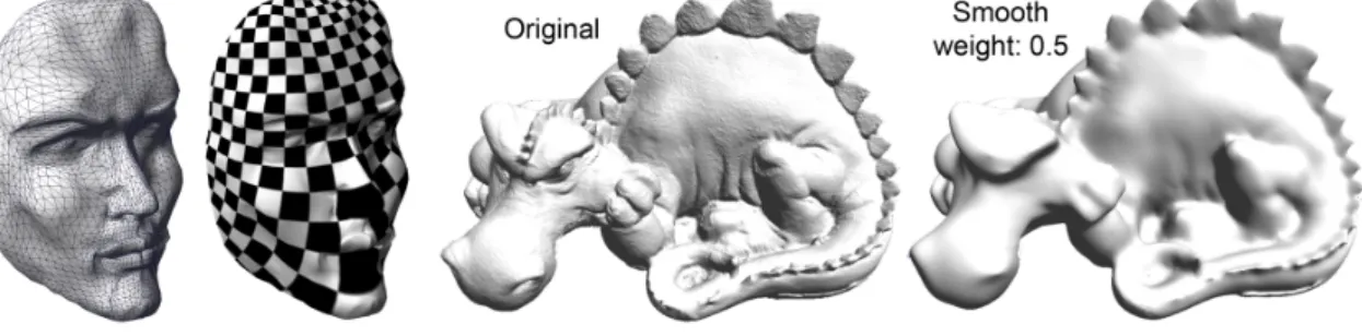
Figure 1: Mesh smoothing computed with our CNC. Left: initial mesh; Center: smoothed mesh; Right: geometry processing with irregular meshes yield matrices with arbitrary non-zero patterns. Consequently, previous dense GPGPU techniques cannot be used, while our CNC implementing a general solver on the GPU can process these irregular matrices.
1
Introduction
1.1 MotivationsIn only a few years, the power of graphics processors has grown to such a point that they now can render realistic complex 3D environments in real-time. Both their computational power and memory bandwidth have significantly overwhelmed CPU specifications. For example, an Intel Quad-Core Xeon 5140 CPU has an observed peak performance of 29 GFlops [19], whereas a modern GPU, like the NVIDIA 9800-GX2, has an observed peak performance of 700 GFlops [7]. Moreover, graphics card manufacturers have recently introduced new dedicated APIs to gen-eral purpose computations on graphics processor units (GPGPU [1]): The Compute Unified Device Architecture (CUDA) from NVIDIA [21] and the Close-To-Metal (CTM) from AMD-ATI [29]. These APIs provide low-level or direct access to GPUs, exposing them as large arrays of parallel processors.
Therefore, numerical solvers, which play a central role in many optimization problems, can be strongly accelerated by using GPUs, at least when low accuracy is acceptable. The key point is parallelizing these algorithms to fit the highly parallel architecture of modern GPUs. As shown in Figure 1, our GPU-based Concurrent Number Cruncher (CNC) accelerates optimization algo-rithms. This paper aims at presenting in greater details the implementation and performance of the CNC, initially introduced in [6], including significant improvements. Our CNC can solve large unstructured problems, based on a very general sparse storage format of matrices, and is designed to exploit the computational capabilities of GPUs to their full extent.
As an example, we demonstrate our solver on two different geometry processing algorithms, namely LSCM [24] (mesh parameterization) and DSI [25] (mesh smoothing). As a front-end to our solver, we use the general OpenNL API [23]; as a consequence, many other geometry processing methods could easily benefit from the CNC [33, 28, 12].
It is known that sparse direct methods are very efficient for geometry processing [5]. In con-trast, in this work, we focus on iterative methods for the following reasons: their memory footprint is much smaller than direct solvers, they can be applied to very large sparse matrices, they are eas-ier to parallelize and implement on the GPU, and, in an interactive context, only a few iterations are needed to update a previous solution. Hence, our CNC implements a Jacobi-preconditioned conjugate gradient solver [17] with Block Compressed Row Storage (BCRS) of sparse matrices on the GPU using both the CTM-API and the CUDA-API (sections 1.2 and 2.1). The BCRS format is much more efficient than the simple Compressed Row Storage format (CRS), by enabling register blocking strategies and vector processing which strongly reduce the required memory bandwidth and computational time [3].
Moreover, we compare our GPU CTM and CUDA implementations of vector operations with several others: a GPU implementation based on OpenGL [22] and the CPU implementations from the Intel Math Kernel Library (MKL) [18] and the AMD Core Math Library (ACML) [2], which are highly multithreaded and SSE3 optimized. For operations involving sparse matrices, we com-pare our GPU implementations with our multithreaded-SSE3 optimized CPU one, since neither the MKL nor the ACML handle the BCRS format. Note that the CUDA BLAS library (CuBLAS) does not provide sparse matrix storage structures.
1.2 The preconditioned Conjugate Gradient algorithm
The preconditioned Conjugate Gradient algorithm is a well known method to iteratively solve a symmetric definite positive linear system [17] (extensions exist for non-symmetric systems, see [32]). As it is iterative, it can be used to solve very large sparse linear systems where direct solvers cannot be used due to their memory consumption.
Given the inputs A, b, a starting value x, a preconditioner M, a maximum number of iterations imax and an error tolerance ε < 1, the linear system expressed as Ax = b can be solved using the
preconditioned conjugate gradient algorithm described as:
i← 0; r ← b − Ax; d ← M−1r; δnew← rTd; δ0← δnew;
while i < imaxand δnew> ε2δ0do
q ← Ad; α ←δnew dTq; x ← x + αd; r ← r − αq; s ← M−1r; δold← δnew; δnew← rTs; β ← δδnew old; d ← r + βd; i ← i + 1; end
In this paper, we present an efficient implementation of this algorithm using the Jacobi pre-conditioner (M = diag(A)) for large sparse linear systems using hardware acceleration through the CTM-API [29] and CUDA-API [21].
1.3 Previous works on GPU solvers and data structures
Depending on the discretization of the problem, solving, for example geometry processing prob-lems, involves band, dense or general sparse matrices. Naturally, different types of matrices lead to specific solver implementations. Most of these methods rely on low-level BLAS APIs that provide basic operations on matrices and vectors.
1.3.1 Iterative solvers Dense and band matrices
The first solvers developed on GPUs were iterative dense or band solvers [22]. This is due to the natural and efficient mapping of dense matrices or band matrices into 2D textures. Most of the work done in this field was for solving the pressure-Poisson equation for incompressible fluid flow simulation by storing matrices into textures. Krüger and Westermann [22] solved this equation using a conjugate gradient based on BLAS operations implemented on the GPU for band matrices.
General sparse matrices
Discretization of optimization problems on irregular meshes leads to solve irregular problems, hence call for a general representation for sparse matrices. Two authors showed the feasibility of implementing the Compressed Row Storage format (CRS). Bolz et al. [4] use textures to store non-zero coefficients of a matrix and its associated two-level lookup table. The lookup table is used to address the data and to sort the rows of the matrix according to the number of non-zero coefficients in each row. Then, an iteration is performed on the GPU simultaneously over all rows of the same size to complete, for example, a matrix-vector product operation. Bolz et al. [4] implemented successfully a conjugate gradient solver and a multigrid solver. Another approach to implement sparse matrices based on the CRS format was proposed by Krüger and Westermann [22], using vertex buffers (one vertex being used for each non-zero element). Krüger and Westermann, as Bolz, provide a conjugate gradient solver. Our CNC also implements general sparse matrices on the GPU, but uses a more compact representation of sparse matrices, and replaces the CRS format with BCRS (Block Compressed Row Storage) [3] to optimize cache usage and enable register blocking and vector computations.
1.3.2 Direct solvers Dense matrices
Direct solvers like Cholesky decomposition [20] and both Gauss-Jordan elimination and LU decomposition [13] have been implemented on the GPU for dense matrices, and proved to be rel-atively efficient when compared to CPU implementations.
General sparse matrices
Implementing a direct solver with sparse data structures involves handling sparse matrices that can be dynamically updated during the solving process. GPUs are not well suited for this purpose, and, to our knowledge, no efficient GPU implementation is available at this time.
1.3.3 New APIs, new possibilities
Previous works on GPGPU used APIs such as DirectX [27] or OpenGL 2.0 [31] to access GPUs and use high-level shading languages such as Brook [8], Sh [26], Cg [11] or GLSL [30] to imple-ment operations. Using such graphics-centric programming model devoted to real-time graphics limits the flexibility, the performance, and the possibilities of modern GPUs in terms of GPGPU.
Both AMD-ATI [29] and NVIDIA [21] recently announced and released new APIs, respec-tively the Close-To-Metal (CTM) and Compute Unified Device Architecture (CUDA) APIs, de-signed for GPGPU. They provide policy-free, low-level hardware access, and direct access to the high-bandwidth latency-masking graphics memory. These new APIs hide graphical functionalities to reduce overheads and simplify GPU programming. In addition to our improved data structures, we use the CTM and CUDA APIs to improve performance.
1.4 Contributions
The Concurrent Number Cruncher (CNC) is a high-performance preconditioned conjugate gradi-ent solver on the GPU using the new GPGPU AMD-ATI CTM and NVIDIA CUDA APIs. The CNC is based on a general optimized implementation of sparse matrices using Block Compressed Row Storage (BCRS) blocking strategies for various block sizes, and optimized BLAS operations
through massive parallelization, vectorization of the processing and register blocking strategies. The CNC was recently introduced [6] for the CTM API only. This paper describes also the CUDA implementation, provides new optimization strategies (efficient usage of the shared memory, ma-trix reordering...) and an in depth comparison with equivalent CPU implemantations. To our knowledge, this is the first linear solver on the GPU that can be efficiently applied to unstructured optimization problems.
2
The Concurrent Number Cruncher (CNC)
The CNC is based on two components: an OpenGL-like API to iteratively construct a linear sys-tem (OpenNL [23], not discussed in this paper) and a highly efficient implementation of BLAS functions on the GPU. The following sections present some usual structures in high performance computing used in the CNC, how we optimized these for modern GPUs and important cache aware implementation features, which proved critical for efficiency.
2.1 Usual data structures in high performance computing
2.1.1 Compressed Row Storage (CRS)
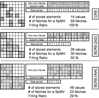
Compressed row storage [3] is an efficient method to represent general sparse matrices (Figure 2). It makes no assumptions about the matrix sparsity and stores only non-zero elements in a 1D-array, row by row. It uses an indirect addressing based on two lookup-tables to retrieve the data:
1. A row pointer table used to determine the storage bounds of each row of the matrix in the array of non-zero coefficients.
2. A column index table used to determine in which column the coefficient lies.
2.1.2 The Sparse Matrix-Vector product routine (SpMV)
The implementation of a conjugate gradient involves a sparse matrix-vector product (SpMV) that takes most of the solving time [32]. This product y ← Ax is expressed as:
for i = 1 to n, y[i] =
∑
j
ai, jxj
Since this equation traverses all rows of the matrix sequentially, it can be implemented efficiently by exploiting, for example, the CRS format (code for a matrix of size n × n):
for i = 0 to n − 1 do y[i] ← 0
for j = row_pointer[i] to row_pointer[i + 1] − 1 do y[i] ← y[i] + values[ j] × x[column_index[ j]] end
end
The number of operations involved during a sparse product is twice the number of non-zero elements of A [32]. Compared to a dense product that takes 2n2 operations, the CRS format therefore significantly reduces processing time for sparse matrices.
2.2 Optimizing for the GPU
Modern GPUs are massively parallel and conform to Single Instruction/Multiple Data (SIMD) ar-chitectures, calling for specific optimization and implementation of algorithms. Several levels of parallelism are offered by GPUs, through multiple pipelines, vector processing and vector read-ing/writing, and several optimizations strategies presented in this subsection.
2.2.1 Multiple pipelines
Multiple pipelines can be used to process data with parallelizable algorithms. In our implemen-tation, each element of y is computed by a separate thread when computing the y ← Ax sparse operation (SpMV). This way, each thread iterates through a row of elements of the sparse matrix A to compute the product.
To maximize performance and hide memory-latencies, the number of threads used must be higher than the number of pipelines. For example, on an NVIDIA G80 which has 128 pipelines grouped by 8 in 16 structures called multi-processors, the size of y should be an order of magnitude higher than 128 elements.
Similarly, operations on vectors, like the SAXPY computing the equation y ← α × x + y, are parallelized by computing one single element of the result y for each thread.
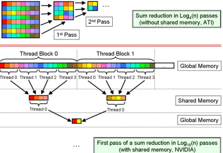
Depending on the targeted GPU, the CNC implements two iterative sum-reductions of the data to parallelize the vector dot product operation (Figure 6). On AMD-ATI GPUs, dot product operations are efficiently done as in [22]: at each iteration, each thread reads and processes 4 scalars and writes one resulting scalar. The original n-dimensional vector is hence reduced by 4 at each iteration until only one scalar remains, after log4(n) iterations. On NVIDIA GPUs, we use a different iterative algorithm taking advantage of the shared memory available on the NVIDIA G80 architecture [21] to reduce more than 4 elements at each iteration per thread. Section 2.3 provides greater details on this dot product implementation.
2.2.2 Vector processing
Some GPU architectures (e.g. AMD-ATI X1k series) process the data inside 4-element vector-processors. This means that a scalar or a read/write operation takes exactly the same time to process as a vector operation on 4 scalar-elements. For such architectures, it is essential to vector-ize the data inside 4-element vectors to maximvector-ize the usage of parallel processors and read/write speed. On a scalar architecture like the NVIDIA G80, data do not need to be vectorized for compu-tations. However, for random memory accesses, it is better to read one float4 than four float1 since the G80 architecture is able to read 128bits in only one instruction. For contiguous read of data, the G80 is able to automatically coalesce the retrieving, removing the need for vectorization of read/write operations. Note that on a CPU it is possible to use SSE1/2/3/4 instructions to vectorize data processing, hence to do simple parallel computations even on a single mono-core CPU.
Since our implementation targets both vector GPU (AMD-ATI X1k series) and scalar GPU (NVIDIA G80) architectures, all operations are vectorized when needed according to the used architecture.
2.2.3 Register blocking: Block Compressed Row Storage (BCRS)
Our CNC uses an efficient implementation of the BCRS format which proved to be faster than CRS on the CPU [3]. The BCRS data structure groups non-zero coefficients in blocks of size BN× BM to maximize the memory fetch bandwidth of GPUs, to take advantage of registers to avoid redundant fetches (register blocking), and to reduce the number of indirections thanks to the reduced size of the lookup tables.
Figure 2: Compressed Row Storage (CRS) and Block Compressed Row Storage (BCRS) examples for the same matrix. The number of stored elements counts all stored elements, useful or not. The number of fetches required to achieve a sparse matrix-vector product (SpMV) is provided for a 4-vector architecture, less fetches being better for memory bandwidth. The filling ratio indicates the aver-age rate of non-zero data in each block, higher filling ratio being better for the computations.
When computing a product of a block spanned over more than one row, it is possible to read only once the associated values from x of the block, to store these values in registers, and reuse them for each row of the block, saving several memory-fetches. Figure 2 illustrates the influence of the block size on the number of fetches. Since our data pattern access is random, fetching and writing scalars 4 by 4 helps in maximizing both read and write bandwidth for either vector or scalar GPU architectures. It is therefore useful to process all four elements of y at the same time, and use blocks of size 4x4. Once the double indirection to locate a block using the lookup-tables has been solved, 4 fetches are required to read a 4x4 block, 1 to read the corresponding 4-scalars of x, and 1 write to output the 4-scalars of the product result into y. Values of x are stored in registers, and reused for each row of the block, which results in fewer fetches than in a classical CRS implementation.
The reduced sizes of the lookup tables reduce memory requirements and, more importantly, the number of indirections to be solved during a matrix operation. Indeed, each indirection results in dependent memory fetches, introducing memory latencies that need to be hidden by the GPU to achieve a good efficiency.
Although a large block size is optimal for register and bandwidth usage, it is adapted only to compact matrices to avoid sparse blocks (Figure 2). A trade-off between the efficiency of large block sizes and a good filling ratio must be set for optimal performance. The CNC implements 2x2 and 4x4 blocks. Small 2x2 blocks are used to handle cases where 4x4 blocks show a very
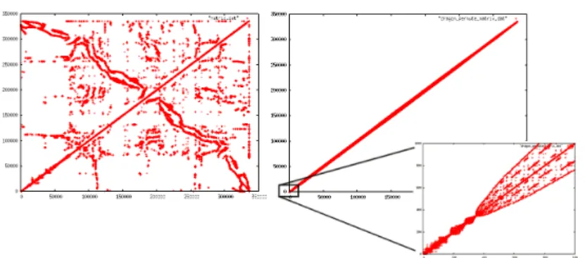
Figure 3: The matrix for smoothing before re-ordering (left) and after RCMK re-ordering (right). Surprisingly, re-ordering does not improve the speed maybe due to GPU’s address scrambling optimized for 2D texture mapping)
low filling ratio. In the SpMV operation for a vector architecture, this 2x2 block size is optimal regarding memory read of the coefficients of the block, but not to read the corresponding x values and to write the resulting y values since only two scalars at a time are read from x and written to y. See section 3 for benchmarks of the BCRS implementation on the GPU.
2.2.4 Reordering for better cache optimality
Reordering is often used when a dense matrix has its rows and columns numbered according to the numbering of the nodes of a mesh. To optimize cache usage, it is possible to use, for example, the Reverse Cuthill McKee (RCMK) reordering heuristic [14, 9]. As shown in Figure 3, the RCMK tries to compress data around the matrix-diagonal, which improves cache-hit when sequentially retrieving data. The CNC implements the RCMK, but our benchmarks showed it had no influence on CPU and both AMD-ATI and NVIDIA GPU implementations. This may be due to special 2D caching strategies, adapted to texture mapping, but not necessarily to numerical computations. Hence, reordering is not used in our performance tests, and not more discussed in this paper.
2.3 Technicalities
2.3.1 The CTM API
The CTM (Close-To-Metal) API is a virtual machine for AMD-ATI X1k or X2k graphics cards [29]. It provides low-level access to both graphics memory and graphics parallel processors. The mem-ory is exposed through pointers at the base addresses of the PCI-Express-memmem-ory (accessible from both the CPU and GPU), and of the GPU-memory (only accessible from the GPU). The CTM does not provide any allocation mechanism, and lets the application fully manage memory. The CTM provides functions to compile and load user assembly codes on the multiprocessors and functions to bind memory pointers indifferently to inputs or outputs of the multiprocessors.
The CNC implements a high-level layer for the CTM hiding memory management by pro-viding dynamic memory allocation (malloc/free like functions) for both GPU and PCI-Express RAM. To optimize the GPU-cache, data pages are automatically aligned on the graphics memory by these allocation functions.
The CNC provides an interface to create and manipulate vectors and matrices on GPUs. Vector or matrix data is automatically uploaded to the GPU memory at their instantiation for later use in BLAS operations. The CNC also pre-compiles and pre-allocates all assembly codes to optimize their execution. To execute a BLAS operation, the CNC binds the inputs and outputs of data on the GPU and calls the relevant assembly code.
Figure 4: Vector and BCRS sparse matrix storage representations on vector architecture GPUs (e.g. AMD-ATI X1k GPUs) with 1D to 2D data rolling.
2.3.2 The CUDA API
The CUDA (Compute Unified Device Architecture) API has the same goals as the CTM API but has a different implementation. It provides a dedicated API for NVIDIA G80 graphics cards [21] that enables low-level direct-access to both graphics memory (called global memory) and graph-ics parallel processors (called stream-processors). The CUDA API exposes the graphgraph-ics memory through pointers that are allocated using specific malloc/free functions. The API provides func-tions to compile/load/execute user programs (called kernels) on the stream-processors. Kernels are written in a high-level C-like language.
On the G80, a structure called processors groups eight stream-processors. Each multi-processor executes only one block of threads at a time, grouping of course a predefined number of threads. A special very fast memory called shared memory is available to each block of threads. It is called shared since all threads of the same block can access the same area of memory and can thus communicate through this memory using synchronized-points in the kernel code avoiding dirty reads or read-write conflicts between threads. This shared memory does not allow communi-cation between blocks of threads, but only between threads of the same block.
As for the CTM API, the CNC implements a high-level layer for NVIDIA GPUs based on the CUDA API. Finally, the CNC uses both CUDA and CTM APIs to provide a unified interface for both optimized BLAS implementations and the conjugate gradient solver.
2.3.3 Data storage structures on vector GPUs (AMD-ATI)
For vector GPU architectures like the AMD-ATI X1K series, the CNC rolls vectors into 2D mem-ory space to benefit from the 2D memmem-ory-cache, and hence can store very large vectors in one chunk (on an AMD-ATI X1k, the maximum size of a 2D array of 4-component vectors is 40962). The BCRS matrix format uses three tables to store the column indices, the row pointers and the non-zero elements of the sparse matrix (Figure 4). The row pointer and column index tables are rolled as simple vectors, and the non-zero values of the matrix are rolled up depending on the block size of the BCRS format. Particularly, the CNC uses strip mining strategies to efficiently implement various BCRS formats. For the 2x2 block size, data are rolled block by block on one 2D-array. For the 4x4 block size, data are distributed into 4 sub-arrays fulfilled alternatively with 2x2 sub-blocks of the original 4x4 block, as in [10]. Retrieving all 16 values of a block can be achieved by four memory fetches from the four sub-arrays at exactly the same 2D index, maximiz-ing the memory fetch capabilities of modern GPUs and limitmaximiz-ing address translation computations.
Figure 5: Vector and BCRS sparse matrix storage representations on scalar architecture GPUs supporting large 1D data array (e.g. NVIDIA G80 GPUs).
2.3.4 Data storage structures on scalar GPUs (NVIDIA)
For scalar GPU architectures like the NVIDIA G80, the CNC stores vectors in a 1D memory space managed by the CUDA API. Very large vectors can therefore be stored continuously in one single array (on the G80, the maximum size of a 1D array is 227). All three tables used in the BCRS format are stored into 1D arrays but in different ways (Figure 5). The row pointer and column index tables are stored as simple 1D vectors, and the nonzero values of the matrix are stored depending on the block size of the BCRS format. Particularly, as for a vector architecture, strip mining strategies are used in the CNC to efficiently implement the different BCRS format. For the 2x2 block size, data are stored block by block on one 1D-array of float4 elements. For the 4x4 block size, the data are distributed into 4 1D-sub-arrays of float4 elements fulfilled alternatively with 2x2 sub-blocks of the original 4x4 block as in [10]. Then, retrieving the 16 values of a block can be achieved by four memory fetches from the four sub-arrays at exactly the same 1D index. As in vector GPUs, this maximizes the memory fetch capabilities and limits the computations of address translations.
2.3.5 Efficient BLAS operations on GPUs
When using an AMD-ATI graphics card and the CTM, the assembly code performing a BLAS operation is made of very “Close-To-Metal" vector instructions such as multiply-and-add (MAD) or 2D memory fetch (TEX). Semaphore instructions can be used to asynchronously retrieve data, helping in a better parallelization/masking of the latencies. The assembly code implementing a sparse matrix-vector product (SpMV) counts about a hundred lines of instructions, and uses about thirty registers. The number of used registers closely impacts performance, so we minimized their use.
On NVIDIA graphics cards with CUDA, the kernel code performing a BLAS operation is made of classical C instructions. The kernel implementing a SpMV on the GPU counts only about forty lines of code, and as for AMD-ATI GPUs, as few registers as possible since their number closely impacts performance.
The SpMV routine executes a loop for each row of blocks of a sparse matrix that can be partially-unrolled to process blocks by pair. For AMD-ATI graphics cards with the CTM, this allows to asynchronously pre-load data and better mask the latencies of the graphics memory, especially for consecutive dependent memory lookups. We increase the SpMV performance by about 30% by processing blocks two by two for both 2x2 and 4x4 block sizes for AMD-ATI GPUs. Conversely, the CUDA API does not provide low-level programming access to asynchronously pre-load data when unrolling this loop. Therefore, this strategy has no impact on the SpMV performance on our CUDA implementation.
Figure 6: Vector sum-reduction parallelizing on a vector architecture without shared memory like AMD-ATI GPUs (top), and on a scalar architecture with shared memory like NVIDIA GPUs (bottom, example for thread-blocks of size 4, hence reducing 4 × 4 = 16 elements at each iteration).
To compute an inner product (SNRM2/SDOT), we use two different methods according to the targeted GPU architecture (Figure 6). As written before, for AMD-ATI GPUs, we use an iterative method as in [22] that reduces, at each iteration, the initial vector size by 4. With NVIDIA GPUs, it is possible to use a more efficient iterative method based on two kernels: one multiplies the components of the vectors and reduces the data set, and the second one just performs the reducing step. In both kernels, each thread of a block has to read four values, reduce them (possibly multiply them), then write the result back into shared memory. In each block of threads, one thread is responsible to sum-up all partial results from the other threads of its block and write back the result in global memory. All the efficiency of the algorithm is conditioned by the choice of the thread block size. Small sizes impose a small reduction factor, hence a large number of iterations, whereas large block sizes impose a small number of iterations but puts a high computational demand on the treads summing up all values stored in shared memory. In our test, the best compromise is obtained for blocks of 128 threads, each reducing 4 values. Thus, at each iteration of the algorithm, the original vector is reduced by 128x4=512 elements. All intermediate reduction steps are performed on temporary memory spaces while the last one uses the memory space specially allocated for the output of the scalar product to maximize performance. Increasing the reduction factor of an iteration also helps reducing the overheads introduced by computations on the GPU.
As the GPU memory is managed by pointers in both CUDA and CTM, outputs of an assembly or a kernel code can be bound to inputs of the next one, avoiding large overheads or useless data copy. In the conjugate gradient algorithm, the CPU program only calls the execution of assembly or kernel codes on the GPU in order, and binds/switches the inputs and outputs pointers. At the end of each iteration, the CPU retrieves only one scalar value (δ) to decide to exit the loop if necessary. Finally, the result vector is copied back to the PCI-Express memory accessible to both the GPU and the CPU in case of using CTM, or copied back to the PC-RAM only accessible to the CPU in case of CUDA. Hence, the whole main loop of the conjugate gradient is fully performed on the GPU without falling back on the CPU for any computations.
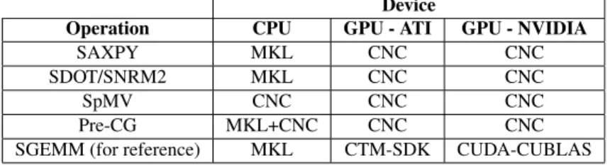
Table 1: Implementations used according to the operation and computing device: CNC is our, MKL is the Intel one, CTM-SDK the AMD-ATI one and CUDA-CUBLAS the NVIDIA one.
Device
Operation CPU GPU - ATI GPU - NVIDIA SAXPY MKL CNC CNC SDOT/SNRM2 MKL CNC CNC SpMV CNC CNC CNC Pre-CG MKL+CNC CNC CNC SGEMM (for reference) MKL CTM-SDK CUDA-CUBLAS
Table 2: Maximum achievable GFlops and GB/s for the used CPU and GPUs.
Device GFlops GB/s CPU 14.6 6.4 GPU - AMD-ATI 240 49.6
GPU - NVIDIA 357 76.8
3
Performance
The preconditioned conjugate gradient algorithm requires a small number of BLAS primitives: a sparse matrix-vector product (SpMV), in our case based on the CRS and BCRS formats, a vector inner-product (SDOT/SNRM2) and vectors operations, e.g. computing the equation y ← α × x + y (SAXPY). This section provides comparisons for these operations in giga floating-point operations per second (GFlops) and percentage of efficiency both for CPU and our two GPU implementations. To be absolutely fair, the provided GFlops integrate all overheads introduced by the computations on the GPU, and count only useful floating-point operations, hence not all performed operations. For example, for a vector of size n, we count the 2 × n − 1 useful operations for an SDOT whatever implementation is used. Table 1 describes the list of implementations used for each operation on each hardware device.
For the SAXPY, SDOT/SNRM2 and SGEMM (dense matrix/matrix multiply, given only for reference) benchmarks on the CPU, we used the Intel Math Kernel Library (MKL) [18] and the AMD Core Math Library (ACML) [2] which are highly multithreaded and optimized using SSE3 instructions. The CPU performance were, on average, close between the MKL and the ACML, hence we choose to only present the results from the former. The SpMV benchmark on the CPU is based on our multithreaded SSE3 optimized implementation, since both the MKL and the ACML do not support the BCRS format. SGEMM on the GPU is based for AMD-ATI graphics cards on the CTM-SDK, and for NVIDIA graphics cards on the CuBLAS library included in the CUDA API. SGEMM is provided only for reference. To show the improvements brought by new APIs like CUDA and CTM, we provide (for reference) benchmarks of the SAXPY and SDOT/SNRM2 op-erations using OpenGL. These OpenGL benchmarks are based on the well known implementation of Krüger and Westermann [22] publicly available.
All benchmarks were performed on a dual-core AMD Athlon 64 X2 4800+, with 2GB of RAM, and with an AMD-ATI X1900XTX with 512MB of graphics memory and an NVIDIA QuadroFX 5600 with 1.5GB of graphics memory. Note that the NVIDIA graphics card is newer than the AMD-ATI, and we naturally get better performance from this card than from the one of AMD-ATI. Table 2 provides the maximum achievable GFlops and GB/s for all devices used in this section.
Benchmarks were performed at least 500 times to average results; they use synthetic vectors for the SAXPY and SDOT/SNRM2 cases, synthetic matrices for the SGEMM case (given for reference), and real matrices built from the set of meshes described in Table 3 for other cases. Figure 7 shows parameterization and smoothing examples of respectively the Girl Face 3 and Phlegmatic Dragon models, both computed using our CNC on the GPU.
Figure 7: Parameterization of the Girl Face 2 and smoothing of the Phlegmatic Dragon using our CNC solver on the GPU.
Table 3: Meshes used for testing matrix operations. This table provides: the number of unknown variables computed in case of a parameterization or a smoothing of a mesh, denoted by #var, and the number of non-zero elements in the associ-ated sparse-matrix denoted by #non-zero (data courtesy of Eurographics for the Phlegmatic Dragon).
Parameterization Smoothing Mesh #var #non-zero #var #non-zero Girl Face 1 1.5K 50.8K 2.3K 52.9K Girl Face 2 6.5K 246.7K 9.8K 290.5K Girl Face 3 25.9K 1.0M 38.8K 1.6M Girl Face 4 103.1K 4.2M 154.7K 6.3M Phlegmatic Dragon 671.4K 19.5M 1.0M 19.6M
Figure 8: SAXPY (y ← α×x+y) and sum-reduction of a vector (SDOT/SNRM2) perfor-mances comparison against the processed vector size between implementations from the INTEL MKL on the CPU, from Krüger and Westermann [22] on the GPU using OpenGL and an NVIDIA graphics card, and from our CNC on the GPU on both AMD-ATI and NVIDIA graphics cards.
3.1 BLAS vector benchmarks
Figure 8 presents benchmarks of SAXPY (y ← α × x + y) and SDOT/SNRM2 (sum-reduction) operations on both CPU and GPU devices.
While the performance curves of the CPU stay steady (around 0.62 GFlops for the SAXPY and 0.94 GFlops for the SNRM2), the GPU performance increases with the vector size. Increasing the size of vectors, hence the number of threads, helps the GPU masking latencies when accessing the graphics memory.
For the SDOT/SNRM2, performance does not increase as fast as for the SAXPY due to its iterative computation that introduces more overheads and potentially more latencies which need to be hidden. Moreover, the slope of the NVIDIA with CUDA curve is stronger for small vector sizes since the corresponding implementation uses a reduction factor of 512 at each reduction step, com-pared to a reduction factor of 4 for ATI-CTM and OpenGL implementation. Thus, with ATI-CTM or OpenGL, more iterations are needed, involving longer cumulated overheads (section 2.3.5).
Note that on an NVIDIA for SAXPY and SDOT/SNRM2 operations, our CNC using CUDA is always faster than the OpenGL implementations. This is due to the reduced overheads and the use of shared memory when available brought by the CUDA API.
At best, on the AMD-ATI GPU, the SAXPY is 12.2 times faster than on the CPU, achieving more than 7.6 GFlops while the SNRM2 is 7.4 times faster achieving 7 GFlops. On an NVIDIA using CUDA (resp. using OpenGL), the SAXPY is 18.0 times faster (resp. 16.4 times) than on the CPU with 11.0 GFlops (resp. 10.0 GFlops), while the SNRM2 is 16.5 times faster (resp. 15.2 times) with 15.5 GFlops (resp. 14.3 GFlops). As expected, NVIDIA performance is higher than AMD-ATI performance due to the generation step between them.
3.2 SpMV benchmarks
Testing operations on sparse-matrices is complicated, since the number and layout of non-zero coefficients strongly govern performance. To test sparse matrix-vector product (SpMV) operations and preconditioned conjugate gradient, we choose five models and two tasks (parameterization and smoothing) which best reflect typical situations in geometry processing (Figure 7 and Table 3).
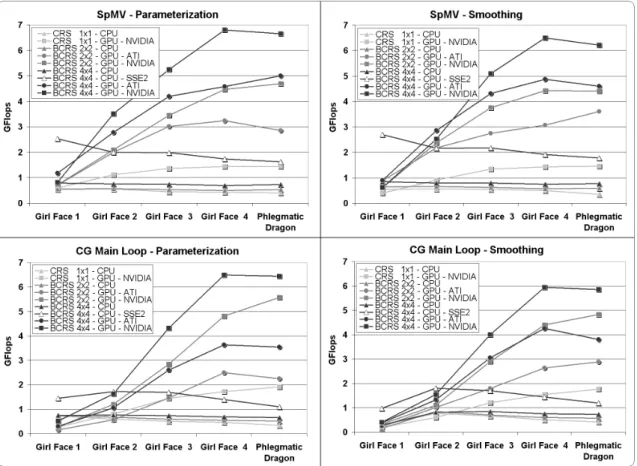
Figure 9 shows the speed of the SpMV for various implementations and applications. Five observations can be made:
1. CPU performance stays relatively stable for both problems while performances of GPUs increase while matrices get larger.
2. Thanks to register blocking and vectorization, BCRS 4x4 is faster than 2x2 (on average 33% and 50% on respectively CPUs -without SSE3- and both GPUs) and the BCRS 2x2 is faster than the CRS (18% and 300% on respectively CPUs and NVIDIA GPUs).
3. AMD-ATI with the CTM (resp. NVIDIA with CUDA) implementation is about 3.1 times faster (resp. 4.0 times) than CPU implementation with multithreaded-SSE3 for significant mesh sizes with BCRS 4x4, achieving at best 5 GFlops (resp. 6.8 GFlops).
4. Multithreaded-SSE3 implementation (enabling vector processing on the CPU) is about 2.5 times faster than standard implementation.
5. For very small matrices, the CNC just compares to CPU implementations, but, in that case, a direct solver would be more appropriate.
Figure 9: Performance curves for the SpMV (sparse matrix-vector product) and the Jacobi-Preconditioned Conjugate Gradient Main Loop. The results are given for CPU standard, CPU multithreaded-SSE3 optimized, and GPU implemen-tations, both for the mesh parameterization and surface smoothing, using CRS (no blocking), BCRS 2x2 and BCRS 4x4.
3.3 Preconditioned Conjugate Gradient benchmarks
Performance for the main loop of a Jacobi-preconditioned conjugate gradient is provided in Fig-ure 9. Since most of the solving time, about 80%, is spent within the SpMV whatever the hard-ware device, the SpMV governs the solver performance, and the comments for the SpMV are also applicable here. GPU solver on AMD-ATI with CTM runs 3.2 times faster than the multithreaded-CPU-SSE3 whereas the one based on NVIDIA with CUDA runs 6.0 times faster. Note that the multithreaded-CPU-SSE3 solver runs 1.8 times faster than the non-SSE3. In the specific case of small matrices, the CNC is not efficient as compared to direct methods which remain relevant.
3.4 Overheads, efficiency and precision
Overheads introduced when copying, binding, retrieving data or executing shader programs on the GPU were the strong bottlenecks of all previous works. The CNC greatly benefit from the CTM and CUDA APIs to this respect; in addition, our implementation has been striving at limiting the number of calls to programs to reduce overheads (section 2.3). During our tests, the total time spent for the processing on the GPU was always higher than 93%, meaning that less than 7% percents were for the overheads, showing a great improvement as compared to previous works. For example, on an NVIDIA graphics card with the CUDA API, the cost of a unique kernel call is around 15 µs.
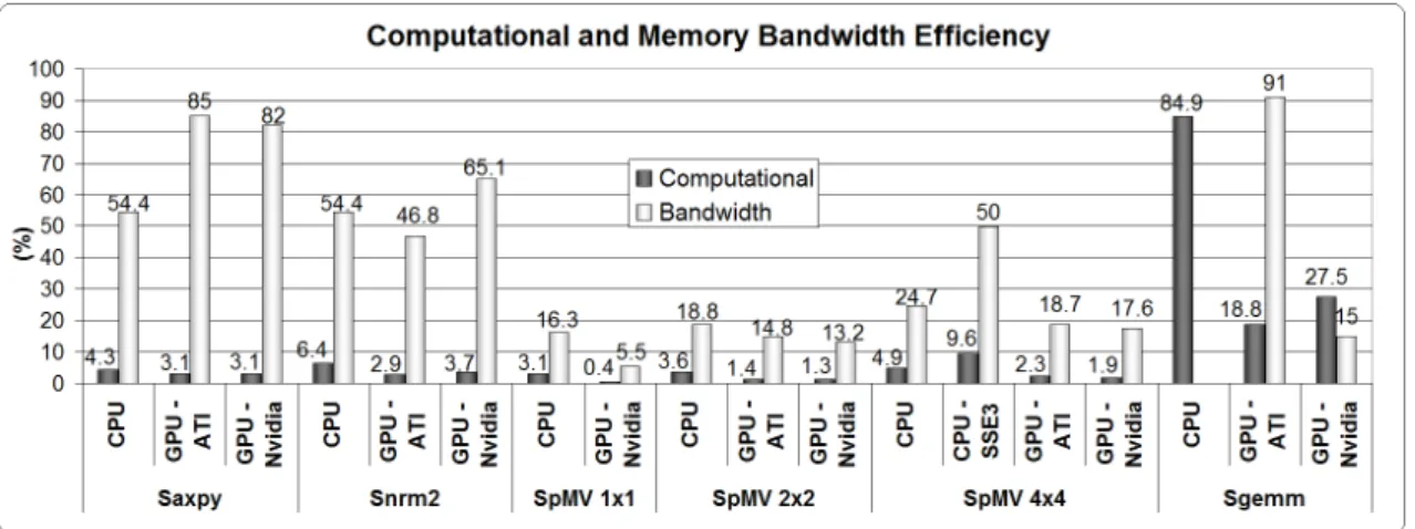
Figure 10: The percentage of computational and memory bandwidth efficiency of dif-ferent operations implemented on the CPU and both AMD-ATI and NVIDIA GPUs for 10242vector size, 10242 dense matrix size and Girl Face 4 model to test the SpMV in case of a parameterization. See Table 1 to determine used implementations. Computational efficiency is calculated per unit of time as the number of operations performed over the achievable maximum number of operations that can be performed on the considered device. Bandwidth ef-ficiency is calculated per unit of time as the consumed bandwidth over the achievable maximum bandwidth. See Table 2 for maximum GFlops and GB/s of the tested devices.
Both CPU and GPU architectures are bound by their maximum computational performance and maximum memory bandwidth. Computational and memory bandwidth efficiencies mainly depend on the tested operations and their implementations as shown in Figure 10. For example, low computational operations as the SAXPY or the SDOT/SNRM2 are limited by the memory bandwidth, and not by the theoretical computational peak power. The SAXPY achieves high bandwidth efficiency on GPUs, higher than 82%, but very low computational efficiency, around 3%.
Conversely, for reference, a dense matrix-matrix product (SGEMM) on the GPU achieves a good computational efficiency of 19% on an AMD-ATI card, and an even better efficiency of 28% on an NVIDIA. In this case, the AMD-ATI implementation achieves very good memory band-width efficiency, near 91%, while the NVIDIA implementation only achieves 15% of efficiency. Those differences are due to implementation “details”. Indeed, the SGEMM is performed by block to benefit from register blocking strategies in both AMD-ATI and NVIDIA implementations. The AMD-ATI implementation uses blocks of size 16x16 while the NVIDIA one uses a size of 32x32. This explains why NVIDIA implementation achieves a better computational efficiency while con-suming less memory bandwidth (so achieves lower bandwidth efficiency) by reducing the number of redundant memory fetches as compared to the AMD-ATI implementation.
In the case of SpMV operations, both computational and memory bandwidth efficiency are low on GPUs and CPUs (although SSE3 greatly helps). This is due to the BCRS format that implies strong cache-miss and several dependent memory fetches. Nevertheless, as previously written, our CNC on the GPU performs the SpMV 3.1 times faster than on the CPU for an AMD-ATI and 4.0 times faster for an NVIDIA.
An important issue for extending the usage of the CNC to other applications is the numerical accuracy of these solvers. Recent graphics cards follow the IEEE-754 standard for single precision
Figure 11: Conjugate gradient relative error in function of the number of iterations to compute a parameterization of the Phlegmatic Dragon model in single preci-sion. The CNC CPU and GPU (NVIDIA) solvers have been used for these tests.
floating point numbers, but with small deviations [21]. Figure 11 shows the relative error of our conjugate gradient solver in single precision on the GPU and the CPU during the iterative compu-tations of a parameterization of the Phlegmatic Dragon model. For the first 500 iterations –where relative error goes down to 10−8 and the solver as already converged– both relative error curves are identical. For the following iterations, the single precision is insufficient to get a more accurate solution on both GPU and CPU devices. The small deviations from the IEEE-754 standard of GPUs are then responsible for the variations relatively to the CPU curve.
While the GPGPU community is waiting for GPU double floating point precision, graphics cards only provide single precision for the moment. For some applications requiring to solve a PDE, single precision may not be enough to fit the required accuracy. Consequently, the cur-rent CNC implementation targets applications which do not require very fine accuracy but very fast performance. Precision issues in solving partial differential equations have been extensively studied in the past few years, particularly when using GPUs as a computational device. Refer-ences [16, 34, 15] provide more details about precision issues in FEM simulations and how to use current GPUs to accelerate double precision computations for higher accuracy. Note that NVIDIA recently announced that their future generation of graphics cards expected before the end of 2008 will support double precision.
4
Conclusions
The Concurrent Number Cruncher aims at providing the fastest possible sparse linear solver through hardware acceleration using new APIs dedicated to GPGPU. It targets applications that do not require very fine accuracy but very fast performance. It uses block compressed row storage, which is faster and more compact than compressed row storage, enabling register blocking and vector processing on GPUs and CPUs (through SSE3 instructions). To our knowledge, this makes our CNC the first implementation of a general symmetric sparse solver that can be efficiently applied to unstructured optimization problems.
Our BLAS operations on the GPU are up to 18 and 16.5 times faster for respectively SAXPY and SDOT/SNRM2 operations than on the CPU using multithreaded-SSE3-optimized Intel MKL library. As compared to our CPU multithreaded-SSE3 implementation, the sparse matrix-vector product (SpMV) is up to 4.0 times faster, and the Jacobi-preconditioned conjugate gradient 6.0 times faster. We show that on any device BCRS-4x4 is significantly faster than 2x2, and 2x2 significantly faster than CRS. Note that our benchmarks include all overheads introduced by the computations on the GPU.
As previously shown, operations on any device are limited either by the memory bandwidth (and its latency), or by the computational power. In most BLAS operations, the limiting factor is the memory bandwidth, which was limited to 49.6 and 76.8 GB/s for respectively our tested AMD-ATI and NVIDIA GPUs. Note that the last generation of AMD-ATI graphics card –the high-end Radeon HD 3870 X2– provides around 120 GB/s of memory bandwidth, which could surely strongly increase the performance of our CNC and the gap with CPU implementations.
Our CNC is currently parallelized for a unique GPU. Hence, we plan to extend the CNC to new levels of parallelism, e.g., across multi-GPUs within a PC (based on SLI or CrossFire configurations), across PC clusters, or within new visual computing systems like the NVIDIA Quadro Plex containing multiple graphics cards with multiple GPUs inside one dedicated box.
We will build and release a general framework for solving sparse linear systems, including full BLAS operations on sparse matrices and vectors, accelerated indifferently by an NVIDIA with CUDA, or by an AMD-ATI with CTM (www.gocad.org>Research>Free Software). Note also that iterative non-symmetric solvers (Bi-CGSTAB and GMRES) can be easily implemented using our framework. We will experiment them in future works as well as the implementation of direct solvers.
5
Acknowledgements
The authors thank the members of the GOCAD research consortium for their support (www.gocad.org), Xavier Cavin, Bruno Stefanizzi from AMD-ATI for providing the CTM API and the associated graphics card, and all the GPGPU team from NVIDIA, especially Tyler Worden, for providing the CUDA API, the associated graphics card and a very useful technical support. We also would like to thank the anonymous reviewers for their valuable comments about our work.
References
[1] GPGPU (General-Purpose computation on GPUs). www.gpgpu.org.
[2] AMD. AMD Core Math Library (ACML). http://developer.amd.com/acml.jsp.
[3] R. Barrett, M. Berry, T. F. Chan, J. Demmel, J. Donato, J. Dongarra, V. Eijkhout, R. Pozo, C. Romine, and H. Van der Vorst. Templates for the solution of linear systems: building blocks for iterative methods, 2nd Edition. SIAM, Philadelphia, PA, 1994.
[4] J. Bolz, I. Farmer, E. Grinspun, and P. Schröder. Sparse matrix solvers on the GPU: conjugate gradients and multigrid. ACM Trans. Graph., 22(3):917–924, July 2003.
[5] M. Botsch, D. Bommes, and L. Kobbelt. Efficient linear system solvers for mesh process-ing. In IMA conference on Mathematics of Surfaces XI, volume 3604 of Lecture Notes in Computer Science, pages 62–83, 2005.
[6] L. Buatois, G. Caumon, and B. Lévy. Concurrent Number Cruncher: An efficient sparse linear solver on the GPU. In High Performance Computation Conference 2007 (HPCC’07). Lecture Notes in Computer Science, 2007.
[7] I. Buck, K. Fatahalian, and P. Hanrahan. Gpubench: Evaluating GPU performance for nu-merical and scientific applications. In Proceedings of the 2004 ACM Workshop on General-Purpose Computing on Graphics Processors, 2004.
[8] I. Buck, T. Foley, D. Horn, J. Sugerman, K. Fatahalian, M. Houston, and P. Hanrahan. Brook for GPUs: stream computing on graphics hardware. ACM Trans. Graph., 23(3):777–786, 2004.
[9] E. Cuthill and J. McKee. Reducing the bandwidth of sparse symmetric matrices. In Pro-ceedings of the 1969 24th national conference, pages 157–172, New York, NY, USA, 1969. ACM Press.
[10] K. Fatahalian, J. Sugerman, and P. Hanrahan. Understanding the efficiency of GPU al-gorithms for matrix-matrix multiplication. In HWWS ’04: Proceedings of the ACM SIG-GRAPH/EUROGRAPHICS conference on Graphics hardware, pages 133–137, New York, NY, USA, 2004. ACM Press.
[11] R. Fernando and M.J. Kilgard. The Cg Tutorial: The definitive guide to programmable real-time graphics. Addison-Wesley Longman Publishing Co., Inc., Boston, MA, USA, 2003. [12] M. S. Floater and K. Hormann. Surface parameterization: a tutorial and survey, pages
157–186. N. A. Dodgson and M. S. Floater and M. A. Sabin, 2005.
[13] N. Galoppo, N.K. Govindaraju, M. Henson, and D. Manocha. LU-GPU: Efficient algo-rithms for solving dense linear systems on graphics hardware. In SC ’05: Proceedings of the 2005 ACM/IEEE conference on Supercomputing, page 3, Washington, DC, USA, 2005. IEEE Computer Society.
[14] N.E. Gibbs, W.G. Poole, and P.K. Stockmeyer. An algorithm for reducing the bandwidth and profile of a sparse matrix. Technical report, College of William and Mary Williamsbourg, VA, Dept of Mathematics, 1974.
[15] D. Göddeke, R. Strzodka, and S. Turek. Accelerating double precision FEM simulations with GPUs. In Proceedings of ASIM 2005 - 18th Symposium on Simulation Technique, Sep 2005.
[16] D. Göddeke, R. Strzodka, and S. Turek. Performance and accuracy of hardware-oriented native-, emulated- and mixed-precision solvers in FEM simulations. International Journal of Parallel, Emergent and Distributed Systems, 2007. accepted for publication November 2006, to appear.
[17] M.R. Hestenes and E. Stiefel. Methods of Conjugate Gradients for solving linear systems. J. Research Nat. Bur. Standards, 49:409–436, 1952.
[18] Intel. Math Kernel Library (MKL). www.intel.com/software/products/mkl.
[19] Intel. Math Kernel Library (mkl) - linpack smp benchmark package. http://www.intel.com/cd/software/products/asmo-na/eng/266857.htm.
[20] J.H. Jung and D.P. O’Leary. Cholesky decomposition and linear programming on a GPU. Scholarly Paper, University of Maryland, 2006.
[21] A. Keane. CUDA (Compute Unified Device Architecture). In http://developer.nvidia.com/object/cuda.html, 2006.
[22] J. Krüger and R. Westermann. Linear algebra operators for GPU implementation of numeri-cal algorithms. ACM Transactions on Graphics (TOG), 22(3):908–916, 2003.
[23] B. Lévy. Numerical methods for digital geometry processing. In Israel Korea Bi-National Conference, November 2005.
[24] B. Lévy, S. Petitjean, N. Ray, and J. Maillot. Least squares conformal maps for automatic texture atlas generation. In ACM, editor, SIGGRAPH 02, San-Antonio, Texas, USA, 2002. [25] J.L. Mallet. Discrete Smooth Interpolation (DSI). Computer Aided Design, 24(4):263–270,
1992.
[26] M. McCool and S. DuToit. Metaprogramming GPUs with Sh. AK Peters, 2004. [27] Microsoft. Direct3d reference. msdn.microsoft.com, 2006.
[28] A. Nealen, T. Igarashi, O. Sorkine, and M. Alexa. Laplacian mesh optimization. In Proceed-ings of ACM GRAPHITE, pages 381–389, 2006.
[29] M. Peercy, M. Segal, and D. Gerstmann. A performance-oriented data-parallel virtual ma-chine for GPUs. In ACM SIGGRAPH’06, 2006.
[30] R.J. Rost. OpenGL Shading Language. Addison-Wesley Professional, 2004.
[31] M. Segal and K. Akeley. The OpenGL graphics system: A specification, version 2.0. www.opengl.org, 2004.
[32] J.R. Shewchuk. An introduction to the conjugate gradient method without the agonizing pain. Technical report, CMU School of Computer Science, 1994. ftp://warp.cs.cmu.edu/quake-papers/painless-conjugate-gradient.ps.
[33] O. Sorkine and D. Cohen-Or. Least-squares meshes. In Proceedings of Shape Modeling International, pages 191–199. IEEE Computer Society Press, 2004.
[34] R. Strzodka and D. Göddeke. Pipelined mixed precision algorithms on fpgas for fast and accurate pde solvers from low precision components. In FCCM ’06: Proceedings of the 14th Annual IEEE Symposium on Field-Programmable Custom Computing Machines (FCCM’06), pages 259–270, Washington, DC, USA, 2006. IEEE Computer Society.