HAL Id: insu-01514409
https://hal-insu.archives-ouvertes.fr/insu-01514409
Submitted on 26 Apr 2017
HAL is a multi-disciplinary open access
archive for the deposit and dissemination of
sci-entific research documents, whether they are
pub-lished or not. The documents may come from
teaching and research institutions in France or
abroad, or from public or private research centers.
L’archive ouverte pluridisciplinaire HAL, est
destinée au dépôt et à la diffusion de documents
scientifiques de niveau recherche, publiés ou non,
émanant des établissements d’enseignement et de
recherche français ou étrangers, des laboratoires
publics ou privés.
in the F2 and the topside ionosphere
Elvira Astafyeva, Irina Zakharenkova, Yann Pineau
To cite this version:
Elvira Astafyeva, Irina Zakharenkova, Yann Pineau. Occurrence of the dayside three-peak density
structure in the F2 and the topside ionosphere. Journal of Geophysical Research Space Physics,
American Geophysical Union/Wiley, 2016, 121 (7), pp.6936-6949. �10.1002/2016JA022641�.
�insu-01514409�
Occurrence of the dayside three-peak density structure
in the F
2and the topside ionosphere
Elvira Astafyeva1, Irina Zakharenkova1, and Yann Pineau1
1
Institut de Physique du Globe de Paris, Paris Sorbonne Cité, Université Paris Diderot, CNRS, Paris, France
Abstract
In this work, we discuss the occurrence of the dayside three-peak electron density structure in the ionosphere. Wefirst use a set of ground-based and satellite-borne instruments to demonstrate the development of a large-amplitude electron density perturbation at the recovery phase of a moderate storm of 11 October 2008. The perturbation developed in the F2and low topside ionospheric regions over theAmerican sector; it was concentrated on the north from the equatorial ionization anomaly (EIA) but was clearly separated from it. At the F2region height, the amplitude of the observed perturbation was
comparable or even exceeded that of the EIA. Further analysis of the observational data together with the Coupled Thermosphere Ionosphere Plasmasphere Electrodynamics model simulation results showed that a particular local combination of the thermospheric wind surges provided favorable conditions for the generation of the three-peak EIA structure. We further proceed with a statistical study of occurrence of the three-peak density structure in the ionosphere in general. Based on the analysis of 7 years of the in situ data from CHAMP satellite, we found that such three-peak density structure occurs sufficiently often during geomagnetically quiet time. The third ionization peak develops in the afternoon hours in the summer hemisphere at solstice periods. Based on analysis of several quiet time events, we conclude that during geomagnetically quiet time, the prevailing summer-to-winter thermospheric circulation acts in similar manner as the storm-time enhanced thermospheric winds, playing the decisive role in generation of the third ionization peak in the daytime ionosphere.
1. Introduction
The equatorial ionization anomaly (EIA), or Appleton anomaly [Appleton, 1954], is a significant feature of the low-latitude ionosphere. The EIA is characterized by two peaks in the F region electron density, located at about 10–15° of latitude from the magnetic equator, and by a trough over the magnetic dip equator. The EIA is primarily driven by a vertical plasma fountain generated by the north-south component of the horizon-tal magneticfield crossed with the horizontal east-west electric field. The resulting vertical E × B drift lifts the plasma to higher altitudes, from where the plasma diffuses downward along the geomagneticfield lines into both hemispheres due to gravitational and pressure gradient forces. The overall process is known as the “fountain effect” [e.g., Kelley, 1989]. During geomagnetic storms, the fountain effect can become a superfoun-tain due to the daytime eastward penetration electricfields and the overall enhancement of the E × B drift force [Kelley et al., 2004; Tsurutani et al., 2004; Mannucci et al., 2005; Astafyeva, 2009a, 2009b].
It has recently been shown that the thermospheric winds play an important role in the development of the ionospheric fountain and superfountain effects [e.g., Balan et al., 2009, 2010]. The role of neutral winds is (1) to reduce (or stop) the downward diffusion of plasma along the geomagneticfield lines, (2) to raise the iono-sphere to high altitudes of reduced chemical loss, and hence (3) to accumulate the plasma at altitudes near and above the ionospheric peak [Balan et al., 2010].
A new instrumental era, with a large number of ground-based instruments installed, along with multi-ple satellite missions operating, allowed to observe new interesting features of the dayside ionospheric beha-vior. For instance, intense geomagnetic storms and superstorms often generate storm-enhanced density (SED) perturbations at high latitudes [e.g., Horvath and Lovell, 2010; Coster et al., 2016], which, in turn, can reach midlatitude regions. The amplitude of such SED can sometimes exceed that of the EIA [e.g., Lei et al., 2015], and to form, therefore a large third and even fourth ionization peaks poleward from the EIA. Besides the storm-time activity, the third ionization peak was shown to occur under geomagnetically quiet conditions caused by solstice-time enhanced thermospheric winds [Valladares, 2013; Maruyama et al., 2016]. It should be noted that such intensive and localized density enhancements can cause disruptions in work of radio
Journal of Geophysical Research: Space Physics
RESEARCH ARTICLE
10.1002/2016JA022641
Key Points:
• We discuss occurrence of daytime three-peak electron density structure as opposed to the conventional two-peak EIA
• During geomagnetic storms, the third ionization peak can occur at equinox. During quiet periods, it is a solstice summer hemisphere feature • Thermospheric meridional winds are
the main driver of the third ionization peak under both quiet and disturbed conditions
Correspondence to:
E. Astafyeva, [email protected]
Citation:
Astafyeva, E., I. Zakharenkova, and Y. Pineau (2016), Occurrence of the dayside three-peak density structure in the F2and the topside ionosphere,
J. Geophys. Res. Space Physics, 121, 6936–6949, doi:10.1002/2016JA022641. Received 4 MAR 2016
Accepted 26 JUN 2016
Accepted article online 29 JUN 2016 Published online 19 JUL 2016
©2016. American Geophysical Union. All Rights Reserved.
communication and navigation systems [e.g., Afraimovich et al., 2009; Rama Rao et al., 2009; Demyanov et al., 2012; Astafyeva et al., 2014; Kelly et al., 2014]; therefore, study of such effects has an importance for all radio-communication system users, in addition to the principal fundamental scientific interest.
The main aim of this work is to study the occurrence of the dayside three-peak electron density structure in the F2region and the topside ionosphere. For this purpose, wefirst provide a detailed multi-instrumental
analysis of the development of a large-scale perturbation near the EIA (i.e., three-peak structure) during a weak-to-moderate geomagnetic storm on 11 October 2008. We discuss possible mechanisms causing such large-scale perturbation. Further, we use the data of the in situ electron density from CHAMP to study the occurrence of the third ionization peak at middle and low latitudes during 2003–2009.
2. Data Set
Our results, both the case-study event of October 2008 and the statistical study, rely on the electron den-sity (Ne) measurements from the planar Langmuir probe instrument on board CHAMP (CHAllenging
Minisatellite Payload) satellite data. CHAMP flew at a near-polar, near-circular orbit with inclination of 87.3° [Reigber et al., 2002] with orbital period of about 91 min. The orbital height of CHAMP changed from 454 km in 2000 to 300 km at the end of 2009 (http://op.gfz-potsdam.de/champ/orbit/index_PRD.html). During the event of 11 October 2008, CHAMPflew at a mean altitude of 330–350 km. For our case-study analysis, we used the ascending (dayside) parts of orbits when the satellite crossed the equator at 14.3 LT. In addition to CHAMP Nedata, for the case-study event of 11 October 2008, we used the following set of
data/instruments: (a) the neutral mass density (ρ) as retrieved from the data of the accelerometer on board CHAMP [Doornbos et al., 2010], (b) maps of vertical total electron content (VTEC) data from dual-frequency ground-based GPS receivers [Rideout and Coster, 2006], (c) data of the F2layer critical frequency (foF2) and of the maximum height (HmF2) from four ground-based ionosonde stations located in North America
[Reinisch and Galkin, 2011], (d) data from Gravity Recovery and Climate Experiment (GRACE) A and B satellites. The uplooking VTEC was calculated from GPS receivers on board GRACE [e.g., Zakharenkova and Astafyeva, 2015]. We also calculate the in situ electron density by using signal measurements of the K-band ranging sys-tem (KBR) between the two GRACE satellites. The technique of the Neretrieval from the KBR measurements
was described in detail by Xiong et al. [2010]. During the October 2008 event, the GRACE satellitesflew at the mean altitude of 455–460 km. We used the descending orbits (the equator crossing time is 13.1 LT), (e) data of VTEC beneath satellite radar altimeter Jason-1. The altimeter’s orbital height is 1336 km and orbital inclination is 66°. For the October 2008 storm study, we used the ascending passes with equator crossing at ~13.8 LT, (f) data of the F2layer peak parameters (NmF2and HmF2) derived from FORMOSAT-3/COSMIC constellation
and GRACE radio occultation profiles.
3. Case-Study Event of 11 October 2008
The year 2008 fell into the period of the solar cycle minimum and also corresponded to the very minimum of the solar and geomagnetic activities from 2006 to 2011 [e.g., Verkhoglyadova et al., 2013].
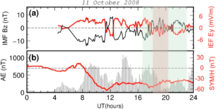
Figures 1a and 1b show the variations of interplanetary and geophysical parameters during the day of 11 October 2008. Although the storm exhibited no classical“sudden commencement,” the magnetic cloud arrived at ~04:50 UT, and the interplanetary magneticfield (IMF) Bz component turned southward from
~06:00 UT and remained that for the next 5 h; it further turned northward for ~1.5 h, and from ~13:00 UT it turned southward for the second time. This second negative Bzevent lasted until ~14:30 UT, when the IMF
Bzstarted to steadily grow up but remained below zero until ~18:00 UT (Figure 1a).
Following these changes in the interplanetary parameters, a moderate geomagnetic storm started on Earth from ~07:30 UT, when the index of geomagnetic activity SYM-H started to monotonely decrease and reached its minimum of 64 nT by ~11:30 UT (Figure 1b). In response to this storm activity, a large positive ionospheric perturbation was observed at middle latitudes in the European region at ~12:00 UT [Zakharenkova et al., 2012]. At 12:50 UT, the SYM-H index increased by ~15 nT, and then decreased again when the IMF Bz turned
negative for the second time, and provoked a second descent in the SYM-H index till its second mini-mum of 57 nT at 17:35 UT (Figure 1b), after which the recovery phase started. Variations of the auroral
electrojet (AE) index showed that this weakly moderate storm was accompanied by strong and long-term substorm activity throughout the whole main phase (Figure 1b). The two large peaks of the enhanced polar magnetic activity occurred at ~09:00–10:00 UT and at ~14:00 UT. The third peak can be seen at ~17:30 UT, i.e., at the beginning of the recovery phase. In our case study, we willfirst focus on the time period from 16:30 to 23:00 UT (shown in light green shaded rectangle in Figure 1). The formation of the third ionization peak next to the EIA was observed from ~18:00 to 20:30 UT (shaded by light red rectangle); this period will be further studied in detail.
3.1. Multi-instrumental Analysis of the Three-Peak Structure on 11 October 2008
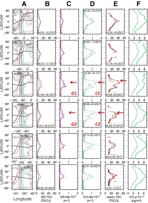
Figure 2 shows the latitudinal profiles of the in situ electron density Neand VTEC as derived from GRACE (Figure 2, columns B and C), CHAMP (Figure 2, column D), and Jason-1 (Figure 2, column E) measurements during the period under consideration. Shortly after the beginning of the last IMF Bz negative event at
16:30 UT, the Neincreased at low and middle latitudes (Figure 2, second line of plots). This effect intensified
by 18:00–19:00 UT (Figure 2, third line of plots). We observed further and stronger increase of the electron density and VTEC in the low-latitude region, as well as at midlatitudes, especially in the north hemisphere (NH), where all three satellites indicated occurrence of a huge perturbation centered around 15°N: GRACE and CHAMP measurements reveal a third ionization peak on the north from the EIA, while in Jason-1 mea-surements the perturbation looks“attached” to the northern EIA crest. During this period of time, one can also notice small TIDs occurring at high latitudes in both hemispheres. The next daytime passes, at ~19:30–20:30 UT, show three-peak structure of the low- and middle-latitude regions even clearer, as the EIA crests moved down along the magnetic equator, while the third peak remained centered around 20°N (Figure 2, fourth line of plots).
Further, from ~21:00 UT, the third peak was less obvious in the satellites’ data (Figure 2, fifth line of plots). Concurrently, the TEC and Newithin the EIA seemed to increase as compared to the previous period of time.
By ~23:00–24:00 UT, we only observe an increase of VTEC and Nein the low-latitude region (Figure 2, the bottom line of plots). The values exceed slightly the quiet time values; however, they are much smaller than those observed at 17:00–21:00 UT.
We would like to emphasize that the observed perturbation was simultaneously seen in data of all the three satellites. This indicates that the low-latitude perturbation was extended from the ionospheric F layer to the lower topside ionosphere. Further careful analysis of the geography of the satellite passes (Figure 2, column A of panels) implies that the perturbation was maximally developed between 70°W and 105°W. However, from only these satellite data it is difficult to get the information on spatial characteristics of the perturba-tion. In addition, due to the longitudinal shift of each successive satellite orbit, it is impossible to track the temporal evolution of the perturbation within a particular area. Therefore, in order to reveal the evolution of the perturbation, we involve data from VTEC maps obtained based on data from ground-based GPS receivers [Rideout and Coster, 2006]. Figures 3a–3d show the variations of the VTEC at low and middle lati-tudes of the northern hemisphere (from 0 to 50°N) as a function of time (in UT), calculated for the range of long-itudes from 90°W (Figure 3a) to 75°W (Figure 3d). Unfortunately, data outside this region were not useful for the analysis. From Figures 3a–3d we can see, first of all, the dayside VTEC increase that occurred from ~16:30 to ~22:30 UT at low and middle latitudes. The northern crest of the EIA with the maximum VTEC up to 50 total Figure 1. Variations of the interplanetary and geomagnetic parameters on
11 October 2008 (from OMNIWeb Plus services, http://omniweb.gsfc.nasa. gov/): (a) interplanetary electricfield (IEF) Eycomponent (Ey, red curve) and
the Bzcomponent of the interplanetary magneticfield (Bz, black curve) and
(b) index of geomagnetic activity SYM-H (red curve) and the geomagnetic auroral electrojet index (AE, gray bars). All parameters are 5 min averaged, except for the period from 06:00 to 07:15 UT, when the IEF Eyand IMF Bzdata
had gaps and were replaced by 1 h data. Light green shaded rectangle delimits the examined period of interest (from 16:30 UT to ~23:00 UT) and red shaded rectangle the time period of the large-scale perturbation observation (from ~18:00 to 20:30 UT).
Figure 2. Variations of ionospheric and thermospheric parameters from ~14:50 to 24:00 UT on 11 October 2008. Vertical TEC (GRACE–magenta curves (column B), Jason-1– brown curves (column E)), the in situ electron density observations (GRACE-magenta curves (column C) and CHAMP–green curves (column D)), and the thermospheric neutral mass density as measured from the CHAMP accelerometer (column F) are compared with the quiet day 9 October (thin curves). The beginning and end time of each satellite pass are written in panels in UT. The trajectories for all the satellites are shown in column A, where black thick curves indicate the position of the magnetic dip equator. GRACE crosses the equator at ~13.1 LT, Jason-1 - at 13.8 LT, and CHAMP at ~14.3 LT. Labels C1, C2, G1, and G2 indicate the same CHAMP and GRACE tracks as in Figure 3e.
electron content unit, 1 TECU = 1016el m 2can be clearly seen around 2–9°N of geographic latitude, which is in agreement with our satellite observations shown in Figure 2. The EIA was maximally developed at ~18:00– 20:00 UT, which corresponds to ~12:00–13:30 LT. Further careful analysis reveals that during this time period, there occurs another VTEC enhancement of ~40–42 TECU that is, depending on longitude, centered around 15–22°N, i.e., ~2–10° of latitude on the north crest of the EIA. At 90–85°W longitudes, the VTEC decreased down to ~35 TECU between the northern EIA peak and the observed third ionization peak.
The relative position of the third ionization peak and the EIA can be better seen from the combined measurements from the ground-based GPS receivers for ~19:15 UT and those by the CHAMP and GRACE satellites during ~18:00–20:00 UT time period (Figure 3e). One can see that the perturbation was elongated along the EIA but also inclined in latitudes: on the west side, it was located farther from the EIA, while on the east side, it was closer to the EIA.
Thus, the ground-based observations confirm our satellite results on development of the low-latitude pertur-bation on the north from the EIA, and they also show that the perturpertur-bation was extended for at least 20° of longitude and remained at quasi-constant position for ~2–2.5 h. To obtain more information on the perturba-tion moperturba-tion in the altitudinal domain, we analyze changes in the ionospheric F2layer peak in around the area of observation of the third ionization peak on 11 October 2008 (Figure 4).
To determine the F2layer peak parameters, the maximum height (HmF2) and the density (NmF2), we use the
vertical electron density profiles from several ionosondes over the considered region, as well as electron Figure 3. (a–d) GPS-VTEC variations on 11 October 2008 as function of UT (from 12:00 to 24:00 UT) and geographic latitude (from 0 to 50 °N), calculated along longitudes from 90 to 75°W with a step of 5° of longitude, and (e) a combination of the GPS-VTEC data for ~19.25 UT and of the electron in situ data Nefrom CHAMP (C1 and C2 passes) and GRACE (G1 and G2)
measurements from Figure 2. C1 pass corresponds to the CHAMP orbit from 18.36 to 19.01 UT and C2 from 19.88 to 20.63 UT. G1 is the GRACE pass from 17.94 to 18.70 UT, and G2 is the pass from 19.05 to 20.27 UT. The three corresponding color scales for the GPS VTEC, CHAMP Ne, and GRACE Nemeasurements are shown on the right of the plot. White triangles show the
density profiles derived from GPS radio occultation experiment on board FORMOSAT-3/COSMIC and GRACE missions. As a reference behavior of the F2peak parameters we consider the model-derived data provided by
the International Reference Ionosphere (IRI) model, which is the international standard for specification of the main ionospheric parameters [e.g., Bilitza et al., 2014]. Maps on Figures 4a and 4b represent the IRI-2016 model-derived NmF2 and HmF2 values as a quiet time reference calculated for 19:00 UT on 10 October 2008. Symbols on the map show the real observations of the F2peak parameters derived from ionosondes
(triangles) at 18:45–19:00 UT and radio occultation profiles (circles), accumulated during 18:20–19:30 UT, for the disturbed day of 11 October 2008. We can note that the measured F2peak parameters agree well with Figure 4. (a and b) Maximum electron density (NmF2) and ionospheric F2maximum height (HmF2) as derived from COSMIC
profiles (circles) and ionosonde (triangles) data for the event of 11 October 2008 at ~19:00 UT. The background colors indicate the background values of the NmF2and HmF2parameters as deduced from the IRI model. The color scale is the
same for measurements from all instruments for NmF2(Figure 4a) and HmF2(Figure 4b). (c–j) Variations of the NmF2
(Figures 4c–4f) and HmF2(Figures 4g–4j) as measured by four ionosonde stations: Millstone Hill, Boulder, Dyess, and Eglin
on the storm day (red squares) and on the day before (black squares). The red shaded rectangles indicate the time of observation of the third ionization peak, the same as in Figures 1 and 5.
the reference map but demonstrate clearly the storm-time changes, which are quite different from the quiet background map. Above 35°N the F2layer peak has relatively small uplift with decrease of the peak density.
At the same time, below 35°N toward the equator the F2layer peak is uplifted more significantly with simul-taneous increase of the peak electron density. For the region close to the occurrence of the third peak (near 15°N–25°N), we have only six radio occultation profiles, which show precisely the strong increase of the F2
peak density together with the layer uplift.
The ionosonde data are shown in Figures 4c–4j. The most southern and the closest to the perturbation sta-tions Dyess and Eglin show dramatic changes in the ionospheric F2layer parameters starting from 16:30 UT, when the negative IMF Bzintensified. At Dyess and Eglin stations, the NmF2increased from ~0.5 × 106cm 3to
~1 × 106cm 3during 3.5 h (Figures 4e and 4f), while at Boulder and Millstone Hill stations, located farther north-westward and north-eastward from the large perturbation, this effect was much less pronounced, as the NmF2remained almost unchangeable (Figures 4c and 4d). At the same time, from 16:30 UT the maximum
F2height increases sharply from 180 to 240 km at Eglin and from 180 to 260 km at Dyess ionosonde stations.
By 19:30–20:00 UT, the HmF2further increased up to 280 km at Eglin and Boulder and reached 300 km at
Dyess. From 20:30 UT, these storm-time enhancements started to decrease (Figures 4g–4j). These observa-tions indicate a significant local ionospheric density increase with concurrent ionospheric uplift close to the area of the third ionization peak. At Millstone Hill ionosonde station, on the northeast from the third ioni-zation peak, the storm-time value did not exceed the quiet-time level.
Unfortunately, data of vertical plasma drifts from these ionosonde stations were not available for this day. Likewise, no data from Millstone Hill, Arecibo, and Jicamarca radars were available. This made it impossible to obtain more details about the vertical plasma displacements that could lead to the formation of the observed third ionization peak.
3.2. Possible Mechanisms Leading to the Development of the Third Ionization Peak on 11 October 2008
It is known that the low-latitude ionospheric behavior is largely determined by E × B drifts, which is the principal driver of the EIA. In turn, the E × B drifts can be affected by prompt penetration of magnetospheric electricfields [e.g., Kelley et al., 1979; Tsurutani et al., 2004], as well as by longer-lived dynamo electric fields resulting from the disturbance neutral winds [Blanc and Richmond, 1980]. In addition to the drifts due to elec-tricfields, traveling atmospheric disturbances (TADs) and storm-time alterations in the global thermospheric circulation causing neutral composition changes have a large impact on the low-latitude ionosphere [Buonsanto, 1999; Fuller-Rowell et al., 1994; Lu et al., 2008; Balan et al., 2010].
Figure 1a shows that the large third ionization peak occurred during small-amplitude variations of the IMF Bz component. Correspondingly, the interplanetary electricfield Ey, calculated using the MHD approximation
from the IMF Bz and the Vxcomponents of the solar wind speed as Bz× Vx(http://omniweb.gsfc.nasa. gov), oscillated between 4 and 2 mV/m. These values are much lower than those during intense geomag-netic storms [e.g., Kelley et al., 2003; Fejer et al., 2007]. Variations of the E × B drifts derived from ground-based magnetometers at Jicamarca and Piura magnetometer stations also show rather small variations of the E × B drift (Figure 5). These observations lead us to conclusion that the electricfield variations were not the princi-pal driver for the three-peak structure to occur.
In absence of direct measurements of the meridional thermospheric winds, we further analyze variations of the neutral mass densityρ along the CHAMP satellite passes at the height of ~340 km (Figure 2, column F). Thefirst increase in the neutral density started shortly after the beginning of the storm at ~06:00 UT (not shown), so by ~16:00 UT the storm-time value of the neutral mass density ~2.5–3 times exceeded the quiet time level at low latitudes. From 16:30 UT, with the new increase of the substorm activity, a new increase of the neutral density occurred at high latitudes and was especially pronounced in the NH during this moment of time. We also note the occurrence of the traveling atmospheric disturbances (TADs) at high latitudes of the NH, which is, most likely, due to the storm-time energy input in the polar region; the perturbations further propagate equatorward and increase the neutral density at low latitudes, reaching the maximum of ~6.5 × 10 12kg/m3at 20:00–21:00 UT. From Figure 2, we conclude on enhanced thermospheric circulation during the considered period of time, especially in the NH, which most likely played a role in the generation of the observed third ionization peak.
3.3. Coupled Thermosphere Ionosphere Plasmasphere Electrodynamics (CTIPe) Simulation Results of the Event of 11 October 2008
In order to support our observational results and to obtain more information about the plasma redistribution within the area of the third peak, here we add results from the Coupled Thermosphere Ionosphere Plasmasphere Electrodynamics (CTIPe) model [Millward et al., 2001; Fuller-Rowell et al., 2002; Codrescu et al., 2012]. CTIPe is a global, three-dimensional, time-dependent, nonlinear code that consists of four distinct components that run concurrently and are fully coupled. Included are a global thermosphere, a high-latitude ionosphere, middle- and low-latitude ionosphere/plasmasphere, and an electrodynamical calculation of the global dynamo electricfield [Codrescu et al., 2012]. The input parameters for the model are (1) fixed time-dependent hemisphere power (GW) and hemispheric power index, (2) ionospheric electric fields from Weimer electrodynamics model for solar wind parameters (density, solar wind velocity magnitude, and clock angle), and (3) F10.7radioflux. The model output contains information on global distribution and numerical
characteristics for neutrals (wind vector; temperature; the density of the three major species O, O2, and N2; and the mean molecular mass) and for ions and electrons (H+, O+, electron density and temperature, height, and electron density of the ionospheric F2peak).
Figure 6 shows the global distribution of the electron density Ne(in color) and of the neutral winds Vn(by
arrows) at the height of 250 km for the time period from 17:30 UT to 20:00 UT. Although the simulation results are not identical to our observational results, the CTIPe model reproduces the occurrence of the three-peak EIA structure in the American and eastern Pacific longitudinal sectors during this period of time. The localized perturbation can be clearly seen at low latitudes in the NH of the American sector, separated from the EIA crests. As in our observations, the perturbation is localized around +10°N, and it is extended for ~30° of longitude. The CTIPe simulations of the thermospheric wind circulation indicate that the third ionization peak was, most likely, formed by the convergence of the winds around this region. On the north of the peak, the winds are equatorward directed, while on the south from it, the winds are poleward from the magnetic equator region.
Vertical distributions of the Neand Vnparameters confirm our conclusions on the role of the thermospheric
winds in the formation of the third ionization peak. Figure 7 shows the development of the third ionization peak at 18:00 UT (Figure 7a) to 19:00 UT (Figure 7b) on the north from the EIA along 255–275°E longitudes. One can also see that the third peak amplitude is comparable with the density within the EIA crests, as in our observations, whereas the amplitudes of the EIA crests are not always equal.
4. Occurrence of the Three-Peak Density Structure: Statistical Results From CHAMP
Above we showed in detail the development of the third peak in the electron density during the recovery phase of a weak geomagnetic storm on 11 October 2008. However, it should be noted that recent advances in modeling show that such dayside three-peak structure can occur during the December solstice time under geomagnetically quiet conditions [Maruyama et al., 2016]. The modeling results by using a new Figure 5. Vertical drift as estimated from horizontal components of magneticfield from the ground-based magnetometers Jicamarca and Piura. Thefigure is from http://jro.igp.gob.pe/english/.
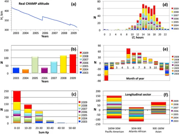
ionosphere-plasmasphere (IP) model for December 2012 case by Maruyama et al. [2016] were supported by observational data from COSMIC occultation data. Before that, Valladares [2013] noticed the occurrence of such “tropical ionization anomaly” over southern hemisphere by using the Low-Latitude Ionospheric Sensor Network (LISN) of ground-based GPS receivers. Therefore, following ourfirst observations, and also considering the rising interest to this topic, here we proceed with analysis of a large data set of the in situ electron density data from CHAMP satellite. For this purpose, we analyze the Nedata for 7 years of observa-tions from 2003 to 2009. As shown in Figure 8a, the orbital height of CHAMP satellite changed from ~415 to ~320 km during these years. Consequently, in 2003–2004 CHAMP sounded higher-altitude atmosphere than in 2008–2009, which might influence the final results of the study of the occurrence of the three-peak EIA during these years, as the EIA is known to be the F2layer feature. Also, due to the CHAMP orbit precession,
the satellite sounds different local sectors during a year. However, analyzing the data set of 7 years elimi-nates this dependence.
Figures 8b–8f summarize the results from our statistical analysis of the CHAMP data for the period from 2003 to 2009. First of all, one can notice that very few three-peak structure events were detected in 2003–2004 and 2006, while many events were found in 2005 and 2008–2009 (Figure 8b). This dependence is, most likely, caused by the changes in the orbital height of CHAMP during the years of observations, as mentioned above (Figure 8a). Thus, in 2003–2004, the CHAMP satellite flew at 380–420 km; then it descended to ~350 km Figure 6. Examples of the three-peak electron density structure as modeled by the CTIPe model from 17:30 UT to 20:00 UT (with time step of 30 min) on 11 October 2008. The electron density (Ne) is shown in color; thermospheric winds (Vn) are shown in arrows. The altitude is taken constant H = 250 km. The color and arrow scales are shown in each plot.
during 2005. At the beginning of 2006, the CHAMP orbital altitude was raised by ~20–25 km. This maneuver, apparently, had a consequence on observations of the three-peak EIA structure by the satellite, as in 2006 we observed less events than in 2005. In 2007–2009 CHAMP gradually descended down to 320 km, and many three-peak EIA events were detected during this time.
Statistical distributions in Figures 8c and 8d demonstrate that the three-peak electron density structure mostly occurs during quiet geomagnetic conditions and in the afternoon hours. The monthly dependence (Figure 8e) shows that the third ionization peak predominantly develops at solstice, while much fewer events were detected in spring/autumn time. From Figure 8e it follows that the three-peak EIA is the summer hemisphere feature, which is in agreement with simulation results by Maruyama et al. [2016]. Our results from Figure 8e are also in line with the main explanation of occurrence of the third ionization peak by pre-vailing neutral meridional windsflowing from summer to winter hemisphere and lifting the plasma along magneticfield lines to higher altitudes where the recombination is slower [Maruyama et al., 2016]. Indeed, the general wind patterns from empirical horizontal wind models HWM07 and HWM14 show the presence of strong equatorward winds throughout the whole summer hemisphere at solstice during the daytime [Drob et al., 2008, 2015]. The strongest meridional equatorward winds occur in the local afternoon hours, Figure 7. Altitudinal distribution of the Ne(in color) and the neutral winds (Vn, white arrows) as obtained from the CTIPe
model simulations at (a) 18:00 UT along longitudes 255–265°E and at (b) 19:00 UT along longitudes 265–275°E, where the three-peak structure was most visible. The arrow scale is the same for all plots; the color scale differs for different plots. The black triangles indicate the latitude of the magnetic dip equator. The red arrows on the top plots show the three peaks, and horizontal dashed lines show the altitude of 250 km, for which the results are shown in Figure 6.
which can explain the local time dependence in Figure 8d. Finally, our statistical results show that the three-peak density structure is more often observed in the American-Pacific regions than at other longitudes (Figure 8f). Comparison of Figures 8e and 8f leads us to conclusion that during NH summer months, the third ionization peak occurs mostly in the American-Pacific region, while during the south hemisphere (SH) summer, it is often observed in the Atlantic-African sector, and in the Asian region, the events occur almost equally in the NH and SH (Figure 8e).
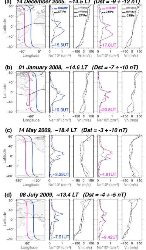
Figure 9 demonstrates the several examples of three-peak events in the Nein situ measurements by CHAMP
during geomagnetically quiet conditions. One can see that during some days several events can be detected by consequent satellite tracks (Figures 9a–9c), while during others (Figure 9d)—only one event is detected and the neighbor satellite track showed the conventional two-peak EIA (blue curve in Figure 9d). In some cases, the third ionization peak can have larger amplitude than the EIA peaks (Figure 9a), and this structure is very similar to that modeled by Maruyama et al. [2016] for December 2012.
It is important to note that modeling the quiet time three-peak density structures is still quite challenging. Maruyama et al. [2016] have used the new advanced IP model to successfully reproduce the occurrence of three-peak density structure during December 2012 solstice conditions. We have run the CTIPe model to see whether it is capable of recreating several quiet-time three-peak EIA events from our database. We have found that the CTIPe model failed to do it, and some examples can be seen in Figure 9. First of all, this can be due to different ways of simulation of the neutral winds in these two models. It is known that the IP model by Maruyama et al. [2016] uses the empirical HWM93 model to obtain the thermospheric wind input for their model, while in the CTIPe model the thermospheric code simulates the neutral atmosphere parameters by numerically solving the nonlinear primitive equations of momentum, energy, and continuity Figure 8. (a) The real CHAMP orbital altitude during the years 2003–2009. (b–f) The occurrence of the three-peak EIA structure as obtained from the in situ Nemeasurements by CHAMP during the period from 2003 to 2009: (Figure 8b)
yearly dependence, (Figure 8c) dependence on the daily index Kp, (Figure 8d) dependence on local time (LT), (Figure 8e) dependence on a month of a year, and (Figure 8f) dependence on longitudinal sector. Colors define the years of observations, as marked on each plot. Negative values N for the number of events in Figures 8e and 8f indicate the occurrence of the third ionization peak in the southern hemisphere.
Figure 9. Examples of the three-peak electron density structures observed by CHAMP during geomagnetically quiet con-ditions. CHAMP satellite trajectories are shown on the leftmost plots, the corresponding Nemeasurements are shown in
blue and magenta lines in the second and fourth columns of plots, and the corresponding UT of the equatorial crossings are shown in colored labels. For comparison, we show in dashed black lines the CTIPe simulation results for the electron density Nealong the real satellite trajectory but at the height of 250 km (around the F2layer). For the same time periods and
geographical position, we show latitudinal profiles of the meridional neutral winds Vnas derived from HWM93 and HWM07
empirical models (gray and thin black lines, respectively) and from the CTIPe model (dashed black lines) in the third and fifth columns. Positive values of Vnsignify the northward direction. The dates, the LT of observations, and the Dst during the
[Fuller-Rowell et al., 2002]. At the same time, from Figure 9 we see that the CTIPe wind profiles are often simi-lar to those by HWM93 and HWM07, which could explain the occurrence of the three-peak structure in some cases, such as shown in Figure 9c. However, in other cases, even though the model wind profiles are similar, they still cannot explain the formation of the third ionization peak caught by observations (e.g., Figure 9a). Second possible reason can be in the fact that the IP model has more accurate representation of the Earth’s magneticfield, which enables more accurate studies of the longitudinal and UT dependencies globally [Maruyama et al., 2016]. Finally, another huge difference between the CTIPe model results and the CHAMP observations is in the fact that the CTIPe model significantly underestimated the electron density: even around the height of the ionization maximum of 250 km, the Nefrom CTIPe is, mostly, much lower than
the Neat the altitude of CHAMP (Figure 9, second and fourth columns of plots). This Neunderestimation, along with incorrect wind profiles and the magnetic field representation, should be the main reasons for the CTIPe model failures to reproduce the quiet-time three-peak density structure. All these demonstrate, therefore, that model improvements are necessary in order to recreate the real ionospheric structure even under geomagnetically quiet conditions.
5. Conclusions
By using the in situ electron density and the VTEC data from GRACE, CHAMP, and Jason-1 satellites that quasi-simultaneously passed in the same 13:00–14:00 LT local region, we observe the development of a large-scale ionospheric perturbation at the recovery phase of the weak geomagnetic storm on 11 October 2008. The per-turbation was concentrated around +10–20°N, i.e., on the north from the equatorial ionization anomaly, and was elongated for at least ~25–30° of longitude. Simultaneous satellite measurements showed that the observed third ionization peak was extended from the ionospheric F2layer up to the low topside ionosphere.
The third peak’s amplitude was comparable or even exceeded that of the EIA crests, especially at the orbital altitude of the CHAMP satellite. The plasma gradients at the poleward boundary of the observed perturbation reached ~1.3 TECU/d, e.g., of latitude (Figure 2), which is comparable with superstorm values [e.g., Astafyeva et al., 2008] and can have a significant space weather impact. The CTIPe model simulations partly reproduced the occurrence of the three-peak Nestructure in the American and Pacific longitudinal sectors from 17:30 UT
to 19:00 UT. The CTIPe thermospheric results helped to reveal that the thermospheric winds served as the principal driver of the observed three-peak EIA structure.
Our analysis of 7 years of the Nedata from CHAMP showed that the three-peak structure occurs during low
geomagnetic activity around the solstice period. The third ionization peak is mostly seen in the afternoon hours in the summer hemisphere. Similarly to the storm-time case study where the enhanced storm-time thermospheric circulation provokes the generation and persistence of the third ionization peak, the quiet time three-peak structures are generated by the prevailing summer-to-winter neutral winds. Our statistical results are in excellent agreement with the study by Maruyama et al. [2016], and, at the same time, our work statis-tically completes their results, as we analyze 7 years of data and provide statisstatis-tically significant contribution. We show that during weak geomagnetic storms and even under low geomagnetic activity, we can observe extreme dayside enhancements in the electron density, which appears as the third ionization peak in addition to the well-known two-peak EIA. Our work, therefore, shows new examples of difficulties for the ionospheric modeling and space weather forecasting.
References
Afraimovich, E. L., E. I. Astafyeva, V. V. Demyanov, and I. F. Gamayunov (2009), Mid-latitude amplitude scintillation of GPS signals and GPS performance slips, Adv. Space Res., 43(6), 964–972, doi:10.1016/j.asr.2008.09.015.
Appleton, E. V. (1954), The anomalous equatorial belt in the F2-layer, J. Atmos. Terr. Phys., 5(1–6), 348–351, doi:10.1016/0021-9169(54)90054-9.
Astafyeva, E. I. (2009a), Effects of strong IMF Bzsouthward events on the equatorial and midlatitude ionosphere, Ann. Geophys., 27,
1175–1187, doi:10.5194/angeo-27-1175-2009.
Astafyeva, E. I. (2009b), Dayside ionospheric uplift during strong geomagnetic storms as detected by the CHAMP, SAC-C, TOPEX and Jason-1 satellites, Adv. Space Res., 43, 1749–1756, doi:10.1016/j.asr.2008.09.036.
Astafyeva, E. I., E. L. Afraimovich, and S. V. Voeykov (2008), Generation of secondary waves due to intensive large-scale AGW traveling, Adv. Space Res., 41(9), 1458–1461, doi:10.1016/j.asr.2007.03.059.
Astafyeva, E. I., Y. Yasukevich, A. Maksikov, and I. Zhivetiev (2014), Geomagnetic storms, super-storms and their impact on GPS-based navigation, Space Weather, 12, 508–525, doi:10.1002/2014SW001072.
Balan, N., H. Alleyne, Y. Otsuka, D. Vijaya Lekshmi, B. G. Fejer, and I. McCrea (2009), Relative effects of electricfield and neutral wind on positive ionospheric storms, Earth Planets Space, 61, 439–445, doi:10.1186/BF03353160.
Acknowledgments
This work is supported by the European Research Council (grant agreement 307998). We acknowledge use of NASA/GSFC’s Space Physics Data Facility’s OMNIWeb service and OMNI data (http://omniweb.gsfc.nasa.gov/) for the data of the interplanetary and geophysical parameters. We thank the Aviso Data Center (http://aviso-data-center.cnes.fr/) for the data of the satel-lite altimeter Jason-1, the GFZ Potsdam for providing GPS data from CHAMP satellite through the ISDC Data Center, and the Physical Oceanography Distributed Active Archive Center (ftp:// podaac.jpl.nasa.gov) for the data of GPS receivers and K-band measurements from the GRACE satellites. We are grateful to the MADRIGAL services for the vertical TEC data (http://cedar. openmadrigal.org/); to the UML DIDBase (http://umlcar.uml.edu/ DIDBase) for the data of Eglin, Dyess, Boulder, and Millstone Hill ionosonde stations. The Eglin station is a part of the USAF NEXION Digisonde network, the NEXION Program Manager is Mark Leahy. We thank the Jicamarca Radio Observatory for the E × B drift data; the UCAR for the radio occultation mea-surements (CDAAC—www.cosmic.ucar. edu); and the IRI Working Group for IRI-2016 program code (irimodel.org). We thank Vadim Paznukhov (Boston College) for his help in the interpreta-tion of the ionograms data and Eelco Doornbos (Delft University) for the data of the neutral mass density from CHAMP. We thank Timothy J. Fuller-Rowell (NOAA/SWPC), Mihail Codrescu (University of Colorado/CIRES and NOAA/SWPC), and Mariangel Fedrizzi (University of Colorado/CIRES and SWPC/NOAA) for their help with the CTIPe model results interpretation. Discussions with Naomi Maruyama (Univerity of Colorado/CIRES and NOAA/ SWPC) were fruitful. The CTIPe simula-tion results were provided by the Community Coordinated Modeling Center (CCMC) at GSFC through their public Runs on Request system (http:// ccmc.gsfc.nasa.gov). The CCMC is a multiagency partnership between NASA, AFMC, AFOSR, AFRL, AFWA, NOAA, NSF, and ONR. We thank Douglas Drob (NRL) for the useful suggestions. This is IPGP contribution 3766.
Balan, N., K. Shiokawa, Y. Otsuka, T. Kikuchi, D. Vijaya Lekshmi, S. Kawamura, M. Yamamoto, and G. J. Bailey (2010), A physical mechanism of positive ionospheric storms at low latitudes and midlatitudes, J. Geophys. Res., 115, A02304, doi:10.1029/2009JA014515.
Bilitza, D., D. Altadill, Y. Zhang, C. Mertens, V. Truhlik, P. Richards, L.-A. McKinnell, and B. Reinisch (2014), The International Reference Ionosphere 2012 - A model of international collaboration, J. Space Weather Space Clim., 4, 1–12, doi:10.1051/swsc/2014004.
Blanc, M., and A. D. Richmond (1980), The ionospheric disturbance dynamo, J. Geophys. Res., 85, 1669–1686, doi:10.1029/JA085iA04p01669. Buonsanto, M. J. (1999), Ionospheric storms—A review, Space Sci. Rev., 88(3/4), 563–601, doi:10.1023/A:1005107532631.
Codrescu, M. V., C. Negrea, M. Fedrizzi, T. J. Fuller-Rowell, A. Dobin, N. Jakowsky, H. Khalsa, T. Matsuo, and N. Maruyama (2012), A real-time run of the Coupled Thermosphere Ionosphere Plasmasphere Electrodynamics (CTIPe) model, Space Weather, 10, S02001, doi:10.1029/ 2011SW000736.
Coster, A. J., P. J. Erickson, J. C. Foster, E. G. Thomas, J. M. Ruohoniemi, and J. B. H. Baker (2016), Solar cycle 24 observations of Storm Enhanced Density and the Tongue of Ionization, in Ionospheric Space Weather: Longitude and Hemispheric Dependencies and Their Solar, Geomagnetic, and Lower Atmosphere Connections, edited by T. J. Fuller-Rowell et al., John Wiley, Hoboken, N. J.
Demyanov, V. V., Y. V. Yasukevich, A. B. Ishin, and E. I. Astafyeva (2012), Effects of ionosphere super-bubble on GPS performance depending on the bubble orientation relative to geomagneticfield, GPS Solutions, 16(2), 181–189, doi:10.1007/s10291-011-0217-9.
Doornbos, E., J. van den IJssel, H. Lühr, M. Förster, and G. Koppenwallner (2010), Neutral density and crosswind determination from arbitrarily oriented multiaxis accelerometers on satellites, J. Spacecr. Rockets, 47(4), 580–589, doi:10.2514/1.48114.
Drob, D., et al. (2008), An empirical model of the Earth’s horizontal wind fields: HWM07, J. Geophys. Res., 113, A12304, doi:10.1029/ 2008JA013668.
Drob, D. P., et al. (2015), An update to the horizontal wind model (HWM): The quiet time thermosphere, Earth Space Sci., 2, 301–319, doi:10.1002/2014EA000089.
Fejer, B. G., J. W. Jensen, T. Kikuchi, M. A. Abdu, and J. L. Chau (2007), Equatorial ionospheric electricfields during the November 2004 magnetic storm, J. Geophys. Res., 112, A10304, doi:10.1029/2007JA012376.
Fuller-Rowell, T. J., M. V. Codrescu, R. J. Moffett, and S. Quegan (1994), Response of the thermosphere and ionosphere to geomagnetic storms, J. Geophys. Res., 99, 3893–3914, doi:10.1029/93JA02015.
Fuller-Rowell, T. J., G. H. Millward, A. D. Richmond, and M. V. Codrescu (2002), Storm-time changes in the upper atmosphere at low latitudes, J. Atmos. Sol. Terr. Phys., 64, 1383–1391, doi:10.1016/S1364-6826(02)00101-3.
Horvath, I., and B. C. Lovell (2010), Storm-enhanced plasma density (SED) features investigated during the Bastille Day superstorm, J. Geophys. Res., 115, A06305, doi:10.1029/2009JA014674.
Kelly, M. A., J. M. Comberiate, E. S. Miller, and L. J. Paxton (2014), Progress toward forecasting of space weather effects on UHF SATCOM after operation Anaconda, Space Weather, 12, 601–611, doi:10.1002/2014SW001081.
Kelley, M. C. (1989), The Earth’s Ionosphere, Academic, New York.
Kelley, M. C., B. G. Fejer, and C. A. Gonzales (1979), An explanation for anomalous equatorial ionospheric electricfields associated with a northward turning of the interplanetary magneticfield, Geophys. Res. Lett., 6, 301–304, doi:10.1029/GL006i004p00301.
Kelley, M. C., J. J. Makela, J. L. Chau, and M. J. Nicolls (2003), Penetration of the solar wind electricfield into the magnetosphere/ionosphere system, Geophys. Res. Lett., 30(4), 1158, doi:10.1029/2002GL016321.
Kelley, M. C., M. N. Vlasov, J. C. Foster, and A. J. Coster (2004), A quantitative explanation for the phenomenon known as storm-enhanced density, Geophys. Res. Lett., 31, L19809, doi:10.1029/2004GL020875.
Lei, J., Q. Zhu, W. Wang, A. G. Burns, B. Zhao, X. Luan, J. Zhong, and X. Dou (2015), Response of the topside and bottomside ionosphere at low and middle latitudes to the October 2003 superstorms, J. Geophys. Res. Space Physics, 120, 6974–6986, doi:10.1002/2015JA021310. Lu, G., L. P. Goncharenko, A. D. Richmond, R. G. Roble, and N. Aponte (2008), A dayside ionospheric positive storm phase driven by neutral
winds, J. Geophys. Res., 113, A08304, doi:10.1029/2007JA012895.
Mannucci, A. J., B. T. Tsurutani, B. A. Iijima, A. Komjathy, A. Saito, W. D. Gonzalez, F. L. Guarnieri, J. U. Kozyra, and R. Skoug (2005), Dayside global ionospheric response to the major interplanetary events of October 29–30, 2003 “Halloween storms”, Geophys. Res. Lett., 32, L12S02, doi:10.1029/2004GL021467.
Maruyama, N., Y.-Y. Sun, P. G. Richards, J. Middlecoff, T.-W. Fang, T. J. Fuller-Rowell, R. A. Akmaev, J.-Y. Liu, and C. E. Valladares (2016), A new source of the mid-latitude ionospheric peak density structure revealed by a new ionosphere-plasmasphere model, Geophys. Res. Lett., 43, 2429–2435, doi:10.1002/2015GL067312.
Millward, G. H., I. C. F. Müller-Wodarg, A. D. Aylward, T. J. Fuller-Rowell, A. D. Richmond, and R. J. Moffett (2001), An investigation into the influence of tidal forcing on F region equatorial vertical ion drift using a global ionosphere-thermosphere model with coupled electro-dynamics, J. Geophys. Res., 106, 24,733–24,744, doi:10.1029/2000JA000342.
Rama Rao, P. V. S., S. Gopi Krishna, J. Vara Prasad, S. N. V. S. Prasad, D. S. V. V. D. Prasad, and K. Niranjan (2009), Geomagnetic storm effects on GPS based navigation, Ann. Geophys., 27, 2101–2110, doi:10.5194/angeo-27-2101-2009.
Reinisch, B. W., and I. A. Galkin (2011), Global ionospheric radio observatory (GIRO), Earth Planets Space, 63, 377–381, doi:10.5047/ eps.2011.03.001.
Reigber, C., H. Lühr, and P. Schwintzer (2002), CHAMP mission status, Adv. Space Res., 30(2), 129–134, doi:10.1016/S0273-1177(02)00276-4. Rideout, W., and A. Coster (2006), Automated GPS processing for global total electron content data, GPS Solutions, 10, 219–228, doi:10.1007/
s10291-006-0029-5.
Tsurutani, B., A. Mannucci, B. Iijima, M. A. Abdu, J. H. A. Sobral, W. Gonzalez, F. Guarneri, and T. Tsuda (2004), Global dayside ionospheric uplift and enhancement associated with interplanetary electricfields, J. Geophys. Res., 109, A08302, doi:10.1029/2003JA010342.
Valladares, C. (2013), LISN: Measurement of TEC values, and TID characteristics over South and Central America, Abstract SA12A-06 presented at 2013 Fall Meeting, AGU, San Francisco, Calif., 9–13 Dec.
Verkhoglyadova, O. P., B. T. Tsurutani, A. J. Mannucci, M. G. Mlynczak, L. A. Hunt, and T. Runge (2013), Variability of ionospheric TEC during solar and geomagnetic minima (2008 and 2009): External high speed stream drivers, Ann. Geophys., 31, 263–276, doi:10.5194/angeo-31-263-2013. Xiong, C., J. Park, H. Lühr, C. Stolle, and S. Y. Ma (2010), Comparing plasma bubble occurrence rates at CHAMP and GRACE altitudes during
high and low solar activity, Ann. Geophys., 28, 1647–1658, doi:10.5194/angeo-28-1647-2010.
Zakharenkova, I., and E. Astafyeva (2015), Topside ionospheric irregularities as seen from multi-satellite observations, J. Geophys. Res. Space Physics, 120, 807–824, doi:10.1002/2014JA020330.
Zakharenkova, I. E., A. Krankowski, I. I. Shagimuratov, Y. V. Cherniak, A. Krypiak-Gregorcyk, P. Wielgosz, and A. F. Lagovsky (2012), Observation of the ionospheric storm of October 11, 2008 using FORMOSAT-3/COSMIC data, Earth Planets Space, 64, 505–512, doi:10.5047/ eps.2011.06.046.