HAL Id: hal-03233475
https://hal.archives-ouvertes.fr/hal-03233475
Submitted on 26 May 2021
HAL is a multi-disciplinary open access
archive for the deposit and dissemination of
sci-entific research documents, whether they are
pub-lished or not. The documents may come from
teaching and research institutions in France or
abroad, or from public or private research centers.
L’archive ouverte pluridisciplinaire HAL, est
destinée au dépôt et à la diffusion de documents
scientifiques de niveau recherche, publiés ou non,
émanant des établissements d’enseignement et de
recherche français ou étrangers, des laboratoires
publics ou privés.
Distributed under a Creative Commons Attribution| 4.0 International License
Wind power potential and intermittency issues in the
context of climate change
Yiling Cai, François-Marie Bréon
To cite this version:
Yiling Cai, François-Marie Bréon.
Wind power potential and intermittency issues in the
con-text of climate change.
Energy Conversion and Management, Elsevier, 2021, 240, pp.114276.
Energy Conversion and Management 240 (2021) 114276
Available online 19 May 2021
0196-8904/© 2021 The Authors. Published by Elsevier Ltd. This is an open access article under the CC BY-NC-ND license (http://creativecommons.org/licenses/by-nc-nd/4.0/).
Wind power potential and intermittency issues in the context of
climate change
Yiling Cai
*, François-Marie Br´eon
Laboratoire des Sciences du Climat et de l’Environnement, LSCE/IPSL, CEA-CNRS-UVSQ, Universit´e Paris-Saclay, 91191 Gif-sur-Yvette, France
A R T I C L E I N F O Keywords: Wind power Load factor Intermittency Spatial de-correlation Climate change A B S T R A C T
Wind power is developing rapidly because of its potential to provide renewable electricity and the large reduction in installation costs during the past decade. However, the high temporal variability of the wind power source is an obstacle to a high penetration in the electricity mix as it makes difficult to balance electricity supply and demand. There is therefore a need to quantify the variability of wind power and also to analyze how this variability decreases through spatial aggregation. In the context of climate change, it is also necessary to analyze how the wind power potential and its variability may change in the future. One difficulty for such objective is the large biases in the modeled winds, and the difficulty to derive a reliable power curve. In this paper, we propose an Empirical Parametric Power Curve Function (EPPCF) model to calibrate a power curve function for a realistic estimate of wind power from weather and climate model data at the regional or national scale. We use this model to analyze the wind power potential, with France as an example, considering the future wind turbine evolution, both onshore and offshore, with a focus on the production intermittency and the impact of spatial de- correlations. We also analyze the impact of climate change.
We show that the biases in the modeled wind vary from region to region, and must be corrected for a valid evaluation of the wind power potential. For onshore wind, we quantify the potential increase of the load factor linked to the wind turbine evolution (from a current 23% to 30% under optimistic hypothesis). For offshore, our estimate of the load factor is smaller for the French coast than is currently observed for installed wind farms that are further north (around 35% versus 39%). However, the estimates vary significantly with the atmospheric model used, with a large spatial gradient with the distance from the coast. The improvement potential appears smaller than over land. The temporal variability of wind power is large, with variations of 100% of the average within 3–10 h at the regional scale and 14 h at the national scale. A better spatial distribution of the wind farms could further reduce the temporal variability by around 20% at the national scale, although it would remain high with respect to that of the demand. The impact of climate change on the wind power resource is insignificant (from +2.7% to − 8.4% for national annual mean load factor) and even its direction varies among models.
1. Introduction
In the context of climate change, air pollution, energy security and depleting fossil fuel reserves, wind power has had a rapid development in the past decade. This rapid development was also favored by decreasing costs. According to the IRERA Renewable Power Generation
Costs 2019 [1], the onshore wind energy installed capacity has increased
from 178 GW to 594 GW from 2010 to 2019 and the offshore wind installed capacity reached 28 GW at the end of 2019. During the same period, the onshore wind LCOE (Levelized Cost of Energy) has dropped from 0.086 $/kWh to 0.053$/kWh, and the offshore wind LCOE has
down from 0.161 $/kWh to 0.115 $/kWh.
However, with the increasing share of wind power in the electricity system, the high variability of this energy source may cause difficulties
to balance production and demand [2,3]. Numerous tools and studies
have been developed to analyze the potential of interconnections, de-mand side management and electricity storage to compensate for the
intermittency [3–6]. For such objectives, analysis at the hourly scale (or
higher) [7–10] is needed to analyze the RES variations and the system
ability to balance supply and demand. Therefore, realistic wind speed data at high spatial and temporal scale is required to simulate the wind power output. The lack of reliable wind speed data at the necessary scale
* Corresponding author.
E-mail address: [email protected] (Y. Cai).
Contents lists available at ScienceDirect
Energy Conversion and Management
journal homepage: www.elsevier.com/locate/enconman
https://doi.org/10.1016/j.enconman.2021.114276
makes it difficult to quantify the potential wind power output, which results in uncertainties in the electricity system planning, in particular
when accounting for the impact of climate change. Reanalysis data [11]
derived from Numerical Weather Prediction (NWP) models and data assimilation methods have been used for such objective. The potential
and limitations of wind power have been analyzed over Sweden [12],
Ireland [13], Great Britain [14], France [[15], p. 5], China [16] and
Europe [17–20] and the globe [21]. However, as pointed out by [11],
weather reanalysis data must be used with caution as several variables show significant biases. Also, the reanalysis data are spatially coarse and are not capable of resolving local variations, especially in complex
terrain and along the coast [22]. Cradden et al [13] confirms, using
MERRA2 reanalysis data, that the agreement between observed and modeled load factors gets better with a larger installed capacity as
averaging statistically reduces the errors. Iain et al. [18] shows the
MERRA and MERRA-2 reanalysis data presents a significant spatial bias in wind speed in different parts of Europe and stress the need to apply a
regional bias correction. Olauson et al [12] demonstrates that the
simulation of Swedish wind power output from numerical weather wind field requires a seasonal and diurnal bias correction; a similar result is
found at the European scale [19]. Gonz´alez-Aparicio et al [17] shows
that unresolved spatial features of the local wind field in reanalysis data leads to underestimate in the highest wind power outputs, and that downscaling the MERRA reanalysis to a much finer spatial scale allows a
better representation of the wind variability. Torralba et al [23] finds a
large spread of wind speed trend for different reanalysis which may
result in biases for wind power estimates. Jourdier [15] shows that the
ERA5 reanalysis provides a better description of the wind field than the MERRA2 model, through a statistical analysis against observations, although it underestimates the wind speeds, in particular over mountain
areas. Gruber et al [24] finds that bias-corrected MEARRA2 with local
measurements and Global Wind Atlas can deliver satisfactory wind simulation result at the regional scale, but not at the local scale; they also
find that ERA5 outperforms MERRA2 [25] in a multi-county application.
European Commission [20] et Bosch et al [21] find combining Wind
Global Atlas with MERRA reanalysis allows a better representation of the wind fields. Although most of the studies are carried out with a specific attention to onshore wind, there are also several studies that
focus on the offshore wind in Iberian Peninsula [26], India [27],
Portugal [28], Spain [29], the north sea [30] and the globe [31]. In the
present paper, we shall focus on the French metropolitan territory because (i) France shows a large variety of terrain and wind pattern and (ii) wind production data are available at the regional scale.
Spatial aggregation reduces the variability of wind power output and is then an effective way to decrease the wind power variability, as
demonstrated in many studies: [32] focuses on China’s and shows that
the regional wind power is highly correlated for some regions, whereas
others show little correlation, as it decreases with the distance; in [33]
the spatial smoothing effects are studied across several EU countries, the result shows that the correlation degree is related to the distance: countries that are close to each other, such as Great-Britain and Ireland, Denmark and Germany, Denmark and Sweden show a strong correlation
in their wind power output; in [19] the short-term variability can be
reduced significantly thanks to the decrease of correlation with
increasing separation distance in Europe. [34] focuses on the Nordic
countries and shows that the wind power outputs in Denmark and
Sweden show the highest correlation. [35] confirms the low correlation
for some countries in Europe that are further apart, which generates some smoothing (less variability) when the total wind power output of the continent is considered. However, none of these studies properly quantify the intermittency mitigation linked to the spatial decorrelation, which is the main concern for real electricity system design. One major
difficulty, as mentioned in [3,36], is the absence of agreed definition of
the “intermittency” and how it can be quantified. Some attempts have
been made in that direction, such as [37] that analyses the wind power
spectral density and its variations with spatial averaging, or [19] that
uses filters to analyze frequency bands containing fluctuations of
different periods, or [38] that computes several metrics of the wind
power density (WPD), such as mean, median and variability, and also considers the temporal length of periods when the WPD in above or below an arbitrary threshold. Other suggestions to quantify the
inter-mittency of wind power are summarized in [3]. They focus on the
sta-tistical variability but do not quantify the rate of change in wind production, although it is an issue for electricity system operation. Another quantification of the intermittency has been recently proposed
[36] by quantifying the spread of the relative deviation of power vari-ation over a time interval, normalized by average power. The wind power intermittency is compared to that of the consumption. These metrics are not sufficient to properly estimate the potential of wind power in a mix, and its potential to replace conventional (thermal) power plants, which is also related to the risk of low wind during periods of high demand. Furthermore, as offshore wind is gaining popularity, thanks to the prospect of higher load factor, reduced variability, and limited opposition from neighbors, it deserves specific attention. In this context, there is a need to better understand and quantify the variability of wind power potential and spatial smoothing effects among regions. We shall therefore use recently-proposed quantification of the inter-mittency to analyze this characteristic of the wind power production that has insufficiently been analyzed.
Due to the prospects of climate change, there are additional un-certainties as the statistics of meteorological conditions may change.
This has already been analyzed for European countries: in [39] the
impact of climate change on the mean load factor is slightly positive in northern and central Europe whereas it appears negative in southern Europe, accompanied by an intensified seasonal patterns at the end of
the century; in [40] the mean wind load factor is found to decrease from
5% to 15% in central and southern Europe by the end of the century in the extreme emission scenario (i.e. RCP8.5), while increase of the same magnitude in some parts of Northern Europe; such northern-southern
divisions are also found in [41,42], where the wind energy source is
projected to increase in Northern-Central Europe while decreases in Mediterranean region at the end of the century; even in the near future (i.e. 2020–2049), the projection is expected to increase 4%-8% in
Northern Europe and to decrease 6%-12% in Mediterranean winter [43];
in [44] a robust and up to 7% increase of wind power output are found at the European scales in the 21st century, and simultaneous production shortfall would be intensified due to more homogenous wind conditions; in [45] the overall annual output change is shown to be less than 5% across the Europe in the 21st century, with larger effects at the very local scale, with negligible variations on the variability; similar conclusions
are found in [46] although there are indications for changes in the
seasonal patterns and variability; in [47] the impact on UK wind power
production is minor in annual production but will affect seasonal
pat-terns and in [48] a mixed impacts are found for UK with an increase in
some region while a decrease in other parts with an intensified inter-
annual variation; in [49] the change in Spain is up to − 8% in mid-
century (2042–2065) for some region and may affect seasonal output.
More studies can be found in Pryor et al [50] which provides a
comprehensive review regarding climate change impacts on wind power
generation besides European countries. [51] stresses that the wind
power potential and its sensitivity to climate change vary between the climate models that are used (both Global Climate Models (GCM) and Regional Climate Models (RCM)) and depends on the bias-correction method, the wind turbine characteristic and implantation. The result-ing uncertainties impact the plannresult-ing of real electricity system. We shall therefore analyze the potential impact of climate change on the wind power production, focusing not only on the averaged load factor as done in previous studies, but also on the other statistical characteristics related to the intermittency.
In this paper, we make use of atmospheric modeling simulations (both weather reanalysis and climate model) to estimate the wind power potential, its intermittency and its sensitivity to climate change, for both
onshore and offshore development. Previous publications cited above have shown significant biases in the wind fields provided by weather models so that there is a need to first develop a bias-correction method that can be applied to both weather reanalysis and climate simulations and also be able to take into account potential wind turbine technology evolution.
We focus on the France region as it offers a large variety of inland terrains, and also offshore potential over the English Channel, the Atlantic and the Mediterranean that cover diverse weather patterns. Although the development in France has not been as fast as that in neighboring countries, the wind installed capacity has increased from 5.8 GW to 16.5 GW in the last decade as revealed by the French
Elec-tricity Balance 2019 report [52]. The French government has announced
ambitious goal for the development of Renewable Energy Source (RES) simultaneously to a reduction of the nuclear share in the mix. In
accordance with the French National Low Carbon Strategy (SNBC) [53]
to reduce its GHG emissions to a quarter by 2050 compared to 1990 with a fully decarbonization in energy sector, the Multi Annual Energy Plan
(PPE) [54] has set up the energy strategy for 2019–2028, which fixed the
goal of wind energy development to achieve 24.1 GW in 2023 and 33.2–34.7 GW in 2028 for onshore, and 2.4 GW and 5.2–6.2 GW in 2023 and 2028 respectively for offshore wind power installations.
In this context, the paper aims at a full evaluation of the wind power potential at the regional and national scale, with France as an example. This evaluation includes the current mean load factor, its potential for improvement with new technologies, and the impact of climate change; the potential contribution of offshore technologies; and a quantitative evaluation of the intermittency at the regional and national scale.
The paper is organized as follows. Section 2 describes the data, and
the method used to estimate the wind power output from potentially-
biased numerical wind field and to quantify the intermittency. Section
3 evaluates the onshore wind power output potential at the French
regional scales and analyses its temporal and spatial variability. For this objective, one uses and evaluates the method (3.1), analyzes the po-tential load factor improvement thanks to the wind turbine evolution (3.2), and discusses the wind power variability and spatial de-
correlations effects (3.3). Section 4 evaluates the offshore wind power
output potential and intermittency effects, by first estimating the offshore wind load factor in French coast with current technologies (4.1), then assessing the potential impact of wind turbine evolution (4.2), and finally by analyzing the intermittency and spatial de- correlation effects, and proposing potential installation distribution
that minimizes the intermittency (4.3). Section 5 focuses on the impact
of climate change in mean and seasonal wind power output and its
intermittency. Section 6 evaluates the performance of different
numer-ical weather wind speed models used in this study so as to discuss the result uncertainty. The last section summarizes the results, discusses the limitations of the study, and suggest further analysis and research.
2. Data and method
2.1. Data
2.1.1. Wind speed data
In this study, we use two different wind speed model data. The analysis weather model aims at providing wind fields that are repre-sentative of the reality at a given time. Conversely, the climate models provide a wind field whose statistic is realistic but with no attempt to represent the reality at a given time.
For the weather model, we use reanalysis dataset, which is derived using multi observations and data assimilations methods. Among different available reanalysis datasets, ERA5 is gaining popularity since its first release in July 2017, and several studies have shown its quality
compared to MERRA-2, [15,22,25,55] which is often used one for wind
power study. Therefore, we use ERA5 reanalysis in our study, which
provides hourly wind speed since 1979 with a spatial resolution of 0.25◦
at 10 m and 100 m altitude. We use the data for 100 m altitude since it is close to the typical wind turbine hub height.
For the climate models, in order to account for model uncertainties in
climate projection [56], we use a number of simulations and two
Representative Concentration Pathways (RCP). These models are developed in the context of the EURO-CORDEX initiative, which
pro-vides regional climate projections for Europe [49]. These high-
resolution simulations are based on low-resolution climate simulation
using various Global Climate Models (GCM models in Table 1) that are
downscaled to higher resolution using Regional Climate Models (RCM in
Table 1). Among the eight different models, six GCM models and three RCM models are included. The combination of GCM and RCM models allow an assessment of the modeling uncertainty. In addition, different GHG emission pathways are studied, where RCP4.5 representative an intermediate scenario, whereas RCP8.5 is a worst-case scenario. Note that the RCM climate simulation that are available for our analysis provide an estimate of the wind speed at 10 m height, whereas the more appropriate 100 m wind speed is not available.
2.1.2. Wind production data
Wind power model development requires empirical data on wind production. Because of commercial rules, the wind power productions are not available at the wind farm scale. Conversely, the French TSO (RTE) makes available hourly onshore wind production data at the
regional and hourly scale since 2013 [57]. In addition, the location and
rated power (capacity) of the wind farms [58] are available.
There are currently no operational offshore wind farms in France. Therefore, we use German offshore production data as a reference. Hourly wind offshore production data from 2016 to 2018 and wind farm implementation in Germany are provided by Open Power System Data
platform [59].
2.2. Methods
The Manufacturer’s Power Curve (PC) for a given wind turbine provide the theoretical load factor as a function of wind speed. However, it does not account for a number of factors, including the representative height of the wind turbine for extracting the model wind speed, the load factor loss due to the wake effects, availability, electrical efficiency, turbine performance, environmental losses, and curtailments. In addi-tion, it is well known that meteorological models present significant biases for the wind speed estimation. These biases may be region- dependent as discussed in the paper cited in the introduction. There-fore, an Empirical Parametric Power Curve Function (EPPCF) method is proposed here to determine a power curve function that is representa-tive of the regional scale and that can be used to generate realistic time series of net wind power load factor from weather and climate model data.
2.2.1. Load factor
The load factor (capacity factor) is defined as the ratio of actual energy output over the rated power over a period and is an indicator of production ability. The load factor time series is computed by regional historical wind power production weighting by wind farm installed
capacity as described in Eq. (1) where h denotes the hour, r denotes
region, LFr,h is the load factor, Er,h is the wind power production, and Pr
is the rated capacity. Note that the wind power production data used in our study is the net production data, which accounts for all loss factors, including the wake effects, availability, electrical efficiency, turbine performance, environmental losses, and curtailments that can be different from one region to another.
LFr,h=
Er,h
2.2.2. Wind speed
We use electricity production data at the regional or national level. The wind speed in the models is provided at a spatial resolution that is higher than the regional/national data of the wind production. Besides, each region contains a number of wind farms. There is therefore a need to compute an effective wind speed that is representative of the regional/national scale. For wind speeds that are lower than the rated wind speed, the wind farm power is roughly proportional to the cubic of the wind speed. We then derive an effective wind speed as described in
Eq. (2) which accounts for the distribution of the wind farms installed capacity within the considered area,
vr,h= (∑ i(v3i,h*pi,h) ∑ ipi,h )1/3 (2) where the sums are over the wind farms considered in the region,
i(lon, lat) indicates the wind farm location, pi is wind power capacity and
v is the model wind speed at the location of the farm.
2.2.3. Empirical Parametric Power Curve Function (EPPCF) model
The method assumes that the load factor is an increasing function of the wind speed. For wind speeds less than a cut-in wind speed, the load factor is close to zero. It then increases following a cubic relationship that saturates to 1. For the largest wind speeds (around 25 m/s), the safety of the wind turbine may impose a blade configuration with no output, but this is an extremely infrequent event that is not considered in our method. As it dominates the recent market, we only consider the pitch-regulated wind turbine that shows a monotonic increase of the output with the wind speed. The method is based on the distribution of wind speeds and load factor. Based on the hypothesis that the load factor is an increasing function of wind speed, the two frequency distributions are used to define the relationship. In other words, the point in the Table 1
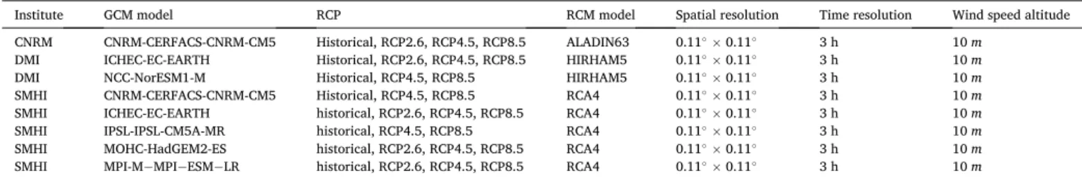
Overview of EURO-CORDEX Climate models used in this study.
Institute GCM model RCP RCM model Spatial resolution Time resolution Wind speed altitude CNRM CNRM-CERFACS-CNRM-CM5 Historical, RCP2.6, RCP4.5, RCP8.5 ALADIN63 0.11◦×0.11◦ 3 h 10 m
DMI ICHEC-EC-EARTH Historical, RCP2.6, RCP4.5, RCP8.5 HIRHAM5 0.11◦×0.11◦ 3 h 10 m
DMI NCC-NorESM1-M Historical, RCP4.5, RCP8.5 HIRHAM5 0.11◦×0.11◦ 3 h 10 m
SMHI CNRM-CERFACS-CNRM-CM5 Historical, RCP4.5, RCP8.5 RCA4 0.11◦×0.11◦ 3 h 10 m
SMHI ICHEC-EC-EARTH historical, RCP2.6, RCP4.5, RCP8.5 RCA4 0.11◦×0.11◦ 3 h 10 m
SMHI IPSL-IPSL-CM5A-MR historical, RCP4.5, RCP8.5 RCA4 0.11◦×0.11◦ 3 h 10 m
SMHI MOHC-HadGEM2-ES historical, RCP2.6, RCP4.5, RCP8.5 RCA4 0.11◦×0.11◦ 3 h 10 m
SMHI MPI-M− MPI− ESM− LR historical, RCP2.6, RCP4.5, RCP8.5 RCA4 0.11◦×0.11◦ 3 h 10 m
Fig. 1. Illustration of the EPPCF method: (a) Wind speed and load factor CDF. (b) EPC obtained by wind speed and load factor CDF match. (c) EPPCF derived by
fitting the EPC using Eq. (3), and manufacturer PPCF derived by fitting manufacturer PC using the same parametric equation which serves as a reference to quantify the deviation of the EPPCF. (d) Future wind turbine adapted EPPCF using current EPPCF adjusted by manufacturer PPCF.
power curve (lf ↔ v) should have the identical probability when
computing the Cumulative Distribution Function (CDF) curve (Fig. 1a).
Hence, by computing the CDF of the model’s wind speed and the observed load factor and matching the two distributions, we can obtain
an Empirical Power Curve (EPC; Fig. 1b). However, it is more practical
to manipulate an analytical function. In addition, there may be some noise in the data which may be smoothed by an analytical fit. For these reasons, we adjust the parameters of an analytical function to fit the EPC and derive an Empirical Parametric Power Curve Function (EPPCF,
Fig. 1c).
The analytical function that we use is
LF(v) =εa* 2 π*arcsin ( 1 − exp [ − ( v c0*εc )k0*εk] ) (3) It computes the load factor as a function of wind speed ν, with three
free parameters (εa, εc, εk). In order to better quantify the power curve
deviation degree compared to a manufacturer’s Power Curve (PC), the parameters are expressed as a standard manufacturer PC shape
param-eters (c0,k0)weighted by coefficients (εc,εk). The nominal value for these
coefficients is 1, and we shall analyze their deviation from this value. Per construction, EPPCF is close to zero for low wind speeds and
saturates to εa for high wind speed. The two other free parameters,
(εc,εk) can be adjusted to fit the shape of the empirical function between
these two extremes, which control the load factor inflection point in wind speed axis and the growth rate of the power curve respectively. When the coefficients vary, the power curve changes in different ways as
illustrated in Fig. 2. In the analysis below, we will see how these
co-efficients vary among regions and meteorological models.
By construction, the load factor that is adjusted by our method has proper statistical properties. Another advantage of this method is that it does not require the load factor and wind speed time series, that are used for the calibration of the function, to be over the same periods, as long as they are long enough to be statistically representative. Also, the EPPCF can be calibrated against current climate values, and then used to esti-mate the load factor from future cliesti-mate simulations. Furthermore, a wind turbine technology improvement, quantified by the change in the manufacturer PC, can also be accounted for through an adjustment of
the EPPCF as illustrated in Fig. 1d.
2.2.4. Technology improvement
One of the objectives of this study is to propose a method that can be used to evaluate future wind power production, accounting for both the change in atmospheric circulation and the improvement of the wind turbines. The EPPCF that can be obtained as described above corre-sponds to the current wind fleet characteristics. In the future, technology will evolve as has been observed in the last decade in rated power, rotor diameter and hub height increase, and a slight decrease in specific
power (i.e. rated power capacity per swept rotor area) [60,61]. Along
with increasing wind turbine hub height, advanced specific power is considered as a promising way to increase load factor and reduce LCOE
cost [60,62–64]. Note that the power curve shape is very sensitive to the
specific power value; a smaller specific power wind turbine reaches the rated power for smaller wind speeds than that with larger specific power
[62]. Since we focus on the load factor, we shall study two important
aspects to measure its potential improvement: (i) the improved power curve shape due to the decrease of specific power (linked to the rotor diameter), and (ii) the increased wind speed due to the increase of hub height. Note that the low specific power wind turbines are designed for sites with low wind speed site, as a larger rotor captures more kinetic energy for such conditions. Conversely, large rotor is poorly suited for sites with high wind speed, as it experiences more mechanic stress in high and turbulent wind conditions. Nevertheless, material improve-ment and better controlling system may make it feasible in the future. In the following, we describe how we account for both the expected decrease in specific power and the expected increase in hub height to correct the EPPCF. As a prior estimate, we use the EPPCF that is derived from the current wind turbine fleet. The impact of the change in specific
power is estimated on the basis of the parameters (c0,k0); i.e. we change
the values from those of the current fleet to those of the expected fleet (manufacturer values). As for the impact of the increased hub height, we
use a traditional power law (Eq. (4)) [65] to estimate the change in
typical wind speed:
v2=v1* ( h2 h1 )α (4)
Where the exponent α is the wind shear coefficient that depends on
the surface roughness and velocity [65,66] as:
α=( z0
h1
)0.2
*[1 − 0.55*log(v1)] (5)
Where v1 is the wind speed corresponding to current hub height h1,
v2 is the increasing wind speed corresponding to a higher hub height h2.
The surface roughness for onshore wind turbines in open flat terrain, grass, few isolated obstacles is approximately 0.03, which could be used as a general surface roughness value in our onshore wind study. The
offshore surface roughness is approximately equal to 0.0061 [67].
In conclusion, an improved EPPCF can be expressed as:
LF(v) =εa* 2 π*arcsin ⎛ ⎜ ⎜ ⎜ ⎝1 − exp ⎡ ⎢ ⎢ ⎢ ⎣− ⎛ ⎜ ⎜ ⎝ v* ( h2 h1 )α c*0*εc ⎞ ⎟ ⎟ ⎠ k*0*εk⎤ ⎥ ⎥ ⎥ ⎦ ⎞ ⎟ ⎟ ⎟ ⎠ (6)
where (εa, εc,εk) are obtained from the current fleet and atmospheric
model adjustment, k*
0 and c*0 are derived from the manufacturer PC and
h1 and h2 are the typical hub heights for the current and future
technologies.
2.2.5. Intermittency and spatial de-correlation quantification metrics
To quantify the regional spatial decorrelation effects, we first investigate the Pearson’s correlation coefficient to statistically measure the linear correlation of wind production time series among regions.
We then use the method proposed by Suchet et al [36] to quantify the
regional/national wind production intermittency. For a given temporal interval Δt, we first evaluate the statistics of the variation P(t +Δt) − P(t) normalized by the mean of P. We define the intermittency as the dif-ference between the 5 and 95 percentiles of the distribution. Low values indicate power stability whereas large values indicate a high variability.
I(Δt) = interpercentile5;95 ({ P(t + Δt) − P(t) P } ) (7) Another indicator of the wind power intermittency, useful for power system planning, is the capacity credit, i.e. the power fraction that can be reasonably expected when needed. The capacity credit is defined in
[68] as “the amount of firm conventional generation capacity that can
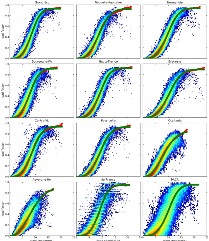
Fig. 3. France onshore wind power curve hourly validation by region. The density histogram shows the ERA5 wind speed at 100 m for the year of 2013–2019
together with the regional wind load factor provided by RTE. The red curve is the EPC derived by matching the wind speed and load factor CDF, whereas the green curve is the fitted curve of EPC using EPPCF method.
be replaced with wind generation capacity, while maintaining the existing levels of security of supply”. A full evaluation of this capacity credit requires a detailed analysis of power system load and wind pro-duction profiles, accounting for the conventional generation capacity, and reliability level. Such analysis is beyond the scope of the paper. In
[68], a simple method focuses on the periods of high demand (highest
10%) and computes the mean wind load factor below the 15 percentile. It provides a quantification of the wind potential during periods of high demand and low wind. This can be done either over the year, or for each month. Here, we make a similar analysis although we search for even calmer (no wind) conditions, i.e. we consider high demand (highest 10% demand) and the lowest 5% wind power percentile. Although this cannot be seen as the true capacity value, it provides a metric that fo-cuses on the most problematic cases of demand-production balance for a high penetration of wind power in the electricity mix.
3. Onshore wind power output potential and intermittency
3.1. Method validation
We simulate the load factor time series for the 12 administrative regions of continental France using the EPPCF method and based on the reported wind load factors and ERA5 reanalysis and EURO-CORDEX data from 2013 to 2019. The simulated result is then compared to the observed data.
3.1.1. Hourly validation
We first look at the ERA5 reanalysis data whose wind field is
representative at a given time. Fig. 3 below illustrates the EPC and
EPPCF compared to historical hourly data of 12 administrative regions in France. The historical scatter plot of load factor as a function of wind speed is based on the observed load factor and a representative regional
wind speed calculated using Eq. (2). It shows the expected shape of a
power curve with a saturation at 0 for low wind and a saturation at a value close to 1 for large winds. There are a few hourly outliers that may result from errors in the atmospheric model or wind power losing fac-tors. For the PACA and Ile de France region, the scatter is larger than for other regions, which is most likely due to the low installed capacity
(<=100 MW). Based on the method described is Section 2.2, we derive
two empirical power curves, here shown in red and green, that, as ex-pected, goes through the data points. The red curve corresponds to the EPC, based on the cumulative histograms of wind speed and load factor,
whereas the green curve shows its analytical fit using Eq. (3). The fit
provides the parameters that are discussed below. In particular, the
saturation value εa shows significant variability among regions, as it
ranges from 0.84 to 0.95. Similarly, the rated wind speed and growth rate of the power curve also show regional variability which is most likely the result of different model bias between regions, due to the surface roughness among other possible causes.
A statistical analysis of the capacity of the empirical model to
reproduce the observed load factors is presented in Table 2. As
mentioned above, the installed capacity in PACA and Ile de France are comparatively low so that the sample is less representative and leads to significant uncertainty in the statistics. Apart from these two regions, the region Auvergne-RA also performs worse than other regions. A large fraction of this region is located in mountain areas, so the complexity of the terrain makes it difficult to estimate a representative wind speed at the regional scale in our method. Apart from the 3 regions mentioned above, the Root Mean Square Error (RMSE) of observed historical versus EPPCF-simulated load factor ranges from 0.055 to 0.068 and the cor-relation varies from 0.93 to 0.97. The observed and simulated regional load factors can also be aggregated at the national scale. The aggrega-tion reduces the statistical noise which leads to significant improvement in the statistics. Indeed, at the national scale, the RMSE is lower than at the regional scale, while the correlation between observed and simu-lated load factors is larger.
We also evaluate the distribution property of the simulated load factor with the whole nation as an example. The statistics of the load factor are important for the planning of the electricity mix with a large share intermittent renewable source, in particular regarding the
fre-quency of periods with very low load factor. As expected, (Fig. 4), the
distribution of the load factor as represented by the analytical model compares well with the empirical distribution. Quantitatively, the fraction of time when the load factor is less than 0.02, 0.05, 0.10 and 0.20 in simulation are 1.5%, 8.8%, 25%, 53.6% compared to 1%, 7.6%, 24.7% and 55.3% respectively.
We then look at EURO-CORDEX models whose statistical property is expected to be realistic but with no attempt to represent reality at a
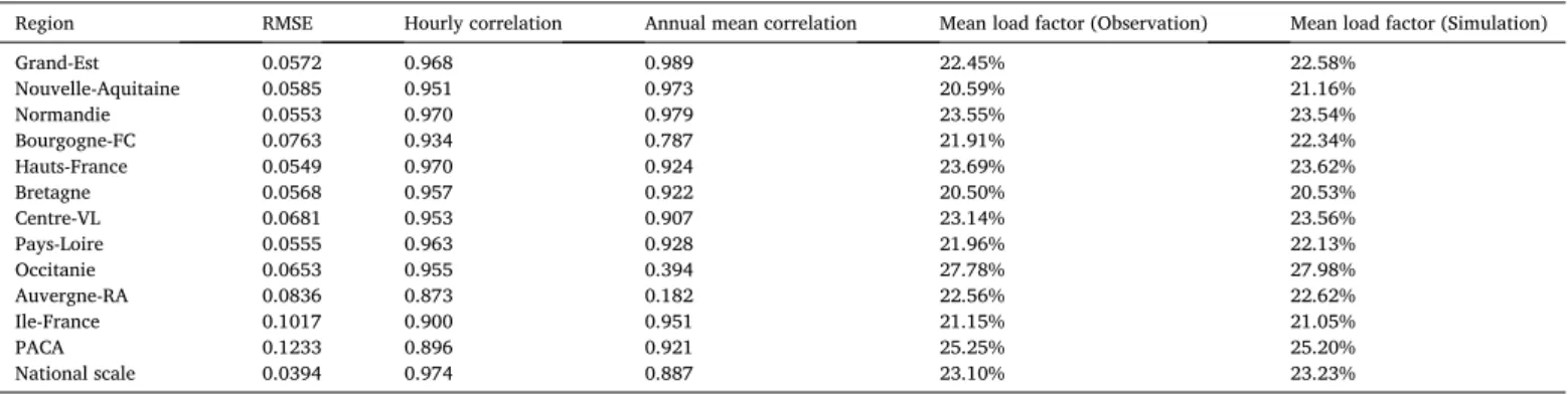
Table 2
Summary of the EPPCF model performance of hourly data from 2013 to 2019. For each region, one provides the RMS difference between the observed and modeled load factor, the hourly and annual mean correlation between these two variables, and the mean load factor, both observed and simulated.
Region RMSE Hourly correlation Annual mean correlation Mean load factor (Observation) Mean load factor (Simulation) Grand-Est 0.0572 0.968 0.989 22.45% 22.58% Nouvelle-Aquitaine 0.0585 0.951 0.973 20.59% 21.16% Normandie 0.0553 0.970 0.979 23.55% 23.54% Bourgogne-FC 0.0763 0.934 0.787 21.91% 22.34% Hauts-France 0.0549 0.970 0.924 23.69% 23.62% Bretagne 0.0568 0.957 0.922 20.50% 20.53% Centre-VL 0.0681 0.953 0.907 23.14% 23.56% Pays-Loire 0.0555 0.963 0.928 21.96% 22.13% Occitanie 0.0653 0.955 0.394 27.78% 27.98% Auvergne-RA 0.0836 0.873 0.182 22.56% 22.62% Ile-France 0.1017 0.900 0.951 21.15% 21.05% PACA 0.1233 0.896 0.921 25.25% 25.20% National scale 0.0394 0.974 0.887 23.10% 23.23%
Fig. 4. The cumulative distribution of observed (black solid line) and simulated
given time. To validate its short-term scale (3 h) statistical property, we compare their distributions and mean load factor to observation. We
only show the national result below. As shown in Fig. 4, all EURO-
CORDEX models show a statistical distribution of the load factor that is well represented by the analytical model, although there are some small differences among models. Quantitively, the average difference of the fraction of time when the load factor is less than 0.02, 0.05, 0.10 and 0.20 in simulations are 0.5%, 3.4%, 3.6% and − 0.8%. The biggest dif-ference we find is the load factor frequency between 0.02 and 0.05 with a small underestimate in the simulation. The average mean in EURO- CORDEX models range from 0.227 to 0.232 compared to 0.231 in observation, which is minimal.
3.1.2. Seasonal-diurnal validation
Wind power presents a significant seasonal and diurnal pattern in observation, it is therefore necessary that the simulated wind can represent well these patterns for the reason that electricity demand also
shows a seasonal and diurnal trend which may somehow different. Fig. 5
shows the combined seasonal and diurnal properties of the whole nation. The left panel compares the simulated wind based on ERA5 reanalysis with observations. The right panel shows the result of EURO- CORDEX model with an example of CERFACS-CNRM-CM5-ALADIN63 in RCP4.5 emission scenario, other EURO-CORDEX models show similar trend. Overall, ERA5 outperforms EURO-CORDEX models in both sea-sonal and diurnal trend. Nonetheless, the seasea-sonal pattern is well replicated in both ERA5 reanalysis and EURO-CORDEX models, with a load factor that is about twice large in winter than it is in summer, with spring and autumn in between. However, the EURO-CORDEX models show a diurnal cycle that is notably different than what is observed; while ERA5 shows a much better agreement with the observations. This
diurnal difference is further discussed in Section 6.
3.1.3. Inter-annual validation
Let us first point out that the observed wind production period (7 years) is somewhat short for a proper inter-annual analysis. Nonetheless, we attempt to evaluate ERA5 inter-annual statistical property by computing the correlation between observed and simulated annual
mean load factor. The result is shown in Table 2. On the whole, most of
the regions present a high correlation between the simulation and observation (i.e. > 0.9). While for some regions, notably in Occitanie and Auvergne-RA where the terrain is complex, the simulation result is not as good. Again, this indicates that ERA5 reanalysis data cannot reproduce accurately the wind field in regions with complex terrain. For EURO-CODDEX models, whose data does not aim at providing real values at a given time, the year-to-year variations are not expected to correlate, although the inter-annual statistical variability can be
compared. The observed inter-annual variability (standard deviation) at the national level for the year of 2013–2019 is 0.01. The EURO-CORDEX models’ inter-annual variability ranges from 0.009 to 0.023, which is therefore larger than what is observed for most models. One should however interpret this result with caution due to the limited time period (7 years) which is insufficient for a proper statistical evaluation.
3.2. Measuring technology improvement
There has been a gradual improvement of wind turbine in the last decade, and this is expected to continue in the future. Therefore, it is important to integrate the wind turbine technology improvement in the near-term and long-term simulation of wind power production. The
reduced specific power is a mean to improve the load factor [63] and
then to decrease the mean cost of wind electricity. Here, we analyze the
impact of technology improvement using the method described in
Sec-tion 2.2.4.
In France, most wind turbine hub height are around 80–100 m, while the rotor diameter varies between 80 m and 110 m, with an average
rated power of around 2.5 MW [73]. We have therefore chosen the wind
turbine model GE 2.5–100, with a hub height of 75/85 m, rotor diameter
of 100 m, rated power of 2.5 MW, and specific power of 318.3 W/m2 as
representative of the current technology. For a representative descrip-tion of the future, we have chosen a wind turbine with 3.75 MW rated capacity, hub height of 115 m, rotor diameter of 130 m and specific
power of 282.5 W/m2 as suggested in [63]. We suppose that in 2020, the
average new installed wind turbine hub-height is 90 m and the specific
power is 318.3 W/m2. These values are extrapolated linearly to 2050.
Assuming that the reduction of the specific power is linear each year, with an average installed wind power capacity of 2 GW each year, along with the current installations, we can estimate the distributions of the wind turbine hub height and specific power in 2030. While in 2050, we only account for the last 25 years installations considering the lifetime of wind turbine. The wind turbine specific power and average hub height
are summarized in Table 3. The correspondent power curve is generated
by a parametric model [69] and is then fitted using the EPPCF model.
Fig. 5. France national onshore wind power seasonal-diurnal validation of ERA5 (left) and CERFACS-CNRM-CM5-ALADIN63 RCP4.5 as an example of EURO-
CORDEX model (right). The dash lines and solid lines are observed and simulated respectively from 2013 to 2019.
Table 3
Summarize of new installed and cumulative wind turbine characteristics in 2020, 2030 and 2050.
2020 2030 2050 New installed hub height (m) 90 115 165 New installed specific power (W/m2) 318.3 282.5 210.9
Mean hub height of installed park (m) 80 93 135 Cumulative specific power (W/m2) 318.3 307.5 253.9
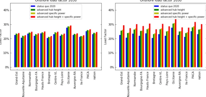
In Fig. 6, we estimate how the average load factor of onshore wind may improve in the near-term (2030) and long-term (2050) future with an advanced hub-height and an advanced specific power in France. The result shows that in the near term, the increased hub-height leads to an improvement of load factor by about 4%, the simulated decrease of specific power similarly leads to an increase of 3%, for a total of 7% (i.e. from 0.231 to 0.246 in absolute at a national level). Assuming that this tendency continues after 2030 (a strong assumption given the un-certainties in further development at this temporal horizon) the national load factor may be improved from 0.231 to 0.301.
3.3. Intermittency and spatial de-correlations
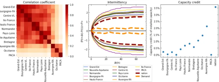
Fig. 7 presents the intermittency and spatial correlation results of the current wind power fleet in France. The left panel shows the Pearson correlation coefficient among regions for onshore wind production. Interestingly, the correlation is close to zero between Mediterranean regions and other regions. Conversely, some regions that are geographically close to each other show a strong correlation (e.g. northeast regions Hauts-de-France and Normandie, northwest regions Grand-Est and Bourgogne-FC, central regions Ile-France and Centre-VL, west and southwest regions Pay-Loire and Bretagne with Nouvelle- Aquitaine). The correlation coefficients decrease with the distance,
which is consistent with the findings of previous studies (e.g. [32–35]).
Fig. 7 (center) quantifies the regional and national intermittency for both the wind power production and the demand. Let us recall that it shows the 5 and 95 percentiles of the relative changes in production. Thus, the curves on the upper part of the figure depict an increasing power, whereas the lower part show cases with a decreasing power. Interestingly, the figure is highly symmetrical, indicating that the large wind power increases are as large as the decreases. As with other results shown above, the results over Ile-de-France and PACA appear less reli-able due to the low number of wind farms in these two regions. The two regions in the south of the country (i.e. Occitanie and Auvergne-RA) show less intermittency than the others. As expected, the aggregation at the national scale does significantly reduce the intermittency. The average regional intermittency can be decreased by 53% for Δt = 1h, 38% for Δt = 6h, 29% for Δt = 24h and 29% for the whole studies period. However, it remains large compared to that of the demand.
Quantitatively, the intermittency metric is ± 15% for national onshore wind production compared to ± 7% for the demand variation for Δt = 1h; ±63% compared to ± 24% for Δt = 6h, and ± 125% compared to ± 16% for Δt = 24h (note that the demand variation at 24 h is lower than it is at 6 h due to the diurnal cycle). These results demonstrate that the intermittency of the wind production is much larger than that of the demand so that the current mid-load and peak-load installations designed to cope with the fluctuations of the demand may not be suf-ficient to face similar variations of the productions if the wind power fleet is developed significantly to replace the baseload nuclear power.
Fig. 7 (right) shows the capacity credit, as defined above, which provides some indication of the minimal wind load factor in conditions of high demand. The regional values are on the order of 1%; Occitanie and Auvergne-RA show the highest value, which is consistent with the previous finding that these two regions are less intermittent than the others. The capacity credit for the national scale (3.6%) remains low but is very much larger than those at the regional scale, which confirms the impact of spatial de-correlation to reduce the intermittency of the wind power production.
A question of interest is whether the intermittency, at the national scale, could be reduced by an optimal spatial distribution of the wind farms. Currently, a large fraction of the wind farms is located in a few regions that show significant correlation. Could a better distribution lead to reduced intermittency? To answer this question, we use four
metrics of the intermittency (i.e. the temporal variability as in Fig. 5b for
Δt = 1, 6, and 24 h, and the capacity credit as defined above). One as-sumes that the wind farm distribution within a region is fixed, but optimize the relative fraction of farms between regions. Compared to the current distribution, the optimization decreases the wind power vari-ability by 14%, 22%, 23% at 1 h, 6 h, 24 h intervals respectively, and increases the capacity credit up to ≈5.5%. Note that the wind farm distribution is rather different from the current situation, and depends
strongly on the optimization criteria (Fig. 8 left). Thus, the positive
impact of region-to-region decorrelation can be optimized so as to reduce the intermittency at the national scale, but the improvement remains modest. In fact, the impact of the spatial distribution on the criteria is so small that the optimization procedure struggles for finding the “best” distribution, and the result may depend on the hypothesis and the period that is chosen for the optimization. One robust result is that
Fig. 6. Load factor improvement including advanced hub-height effect (green bar), advanced specific power effect (yellow), and combined effects of hub-height and
specific power improvement (red), compared to current status in 2020 (blue), as derived from EPPCF model using ERA5 reanalysis wind speed data for regional and national onshore wind in 2030 (left), and 2050 (right).
the wind production in southern regions is less variable than in the North, so that more wind farms should be installed there when aiming at a more stable production. Another robust result is that the variability of the wind production, at the national scale, remains high, even for an optimized distribution. Finally, we acknowledge that this analysis is rather theoretical as the placement of wind farms are limited by factors other than the national production optimization, such as the maximized yearly production of the wind farm, land availability and social acceptance.
4. Offshore wind power output potential and intermittency
4.1. Load factor estimation
There are currently no operational offshore wind farms in France. We therefore do not have empirical power production data representative of the French coasts. To calibrate the relationships between modeled wind
speed and wind power production (i.e. the EPPCF), we shall therefore use data available for the German coasts, but corrected by country- specific wind turbine generation profile. According to the Germany
offshore wind energy development status report [70], at mid-2019,
Germany offshore wind turbine has an average hub height of 94 m,
rotor diameter of 130 m, and specific power of 368 W/m2. In France, the
Saint-Nazaire offshore wind project uses GE Haliade 150–6 MW wind turbine (hub height: 100 m, rotor diameter: 150 m, rated power: 6 MW,
and specific power: 335.9 W/m2). We shall use the characteristics of this
turbine to analyze the potential of offshore wind production in France. We first apply the EPPCF method to the wind farms off the coast of Germany, which allows an empirical estimate of the offshore power curve, with respect to the modeled wind. The validity of the empirical function can be compared to the true load factor at the hourly scale. The accuracy of the empirical fit is acceptable, with an RMSE of 0.10 and a
correlation of 0.93. The comparison plots (Fig. 9) confirm the fair
agreement between the modeled and measured load factor but show that Fig. 7. Onshore wind intermittency and spatial decorrelation current state quantification. Pearson correlation coefficients of onshore wind load factor time series
among regions (left). Regional wind load factor (solid line), national wind load factor (dashed line in darkred) and national demand (dashed line in orange) intermittency quantification with regard to rapidity and amplitude of wind power variation; namely, the 5th and 95th percentile of relative wind load factor or demand change relative to average wind load factor or demand at intervals (Δt) from 1 h to 70 h (center). Regional and national onshore intermittency quantification with regard to equivalence of ‘firm’ capacity in long-term system planning; namely, the capacity credit measured by the average load factor exceeding 95th percentile over top 10% load periods (right). The data is based on hourly historical observations from 2013 to 2019 provided by RTE.
Fig. 8. Results of the optimization of the Onshore wind regional distribution aiming at a reduction of the national production intermittency, based on different
metrics (i.e. Metric1: lowest relative wind power change for Δt = 1, Metric2: same as metric1 but for Δt = 6, Metric3: same as metric1 but for Δt = 24, Metric4: highest capacity credit). Left: Regional distribution of the installed capacities for the present and the various criteria. Center: Representation of the intermittency for the current and the optimized distribution. Right: Capacity credit for the current and optimized distributions.
the model often leads to large over-estimates in case of strong wind. The most likely hypothesis for these overestimates is curtailment of the wind farms for protection when a storm affects the area. These cases with high wind speeds are rare, so that the impact on the overall statistic is not significant.
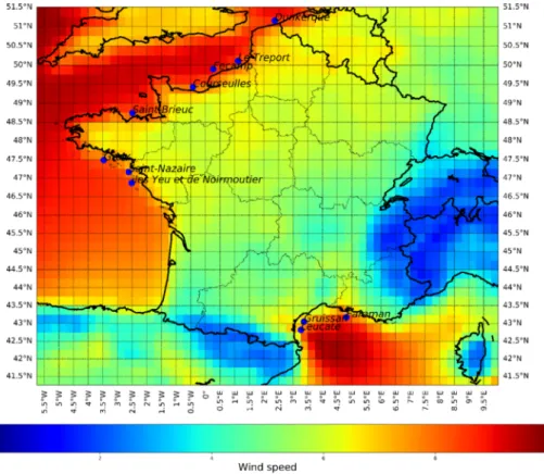
For the development of offshore wind power in France, several sites are considered in the English Channel, the Atlantic, and the
Mediterra-nean, as shown in Fig. 10. The potential developments in the
Mediter-ranean are not as advanced as those over the west coast because the waters are deeper which then requires the use of a floating technology, which is less mature than the grounded technology.
The EPPCF that was calibrated against the offshore wind farms of Germany is then applied to the modeled wind at the location of wind projects off the coast of France. Both ERA5 reanalysis and EURO- CORDEX modeled wind are used. One may question the ability of the model to accurately reproduce the wind gradient close to the coast. In
addition, ERA5 and EURO-CORDEX have a spatial resolution of 0.25◦
and 0.11◦ respectively, which is similar or larger than the typical
dis-tance of the offshore wind farms to the coast (around 15 km). As a consequence, the model wind may be representative of a surface that contains both land and sea surface. We therefore investigate how the distance to the coast impacts the calculated mean load factor. This also appears necessary as offshore wind installations may be further away from the coast in the future. We therefore analyzed how the mean load factor increases as the wind farm location is moved away from the coast in the model. For ERA5, we simulated locations away from the original
position 1 and 2 times the 0.25◦spatial resolution (i.e. 28 km and 56 km)
and searched for the highest value. For EURO-CORDEX models, we used a similar procedure but with 5 distances (i.e. 12 km, 24 km, 36, 48 km and 60 km).
Fig. 11 shows the results of this analysis. First, there is a large dispersion among the EURO-CORDEX models with a full range of low factor that is close to 0.1, for a mean value of 0.36. Second, the load factor increases, as expected as the theoretical location of the wind farm moves away from the coastline.
There is evidence for outliers in the load factor derived from the costal wind speed in EURO-CORDEX models. Some of the load factor computed for the true location of the wind farm, where the distance to the coast is on average 15 km, are surprisingly low, as for Saint-Nazaire according to ERA5 (25%), the Dunkerque site according to IPSL-CM5A- MR-RCA5 (<22%) and most sites according to HadGEM2-ES-RCA5. Most of ERA5 derived load factors are around 30%, and do not exceed 34%. The load factors from the EURO-CORDEX ensemble of models are quite dispersed, and the median load factors for most sites are below 30%. As expected, the load factors increase with the distance from the coastline. The estimates based on the ERA5 simulation increase from Fig. 9. Comparison of the observed and modeled load factor for offshore wind
power off the coast of Germany. The colored scatterplot is a density histogram of reported load factor and ERA5 wind speed at 100 m for the year of 2016–2018; the red curve is the derived EPC by matching the wind speed and load factor CDF; the green curve is the EPPCF method obtained though the best fit procedure.
30.5% to 35.1% in average with an addition grid move (28 km) from its original location. The EURO-CORDEX increases from 28.2% to 33.7% in average of 1st quartile, from 30.9% to 35.9% in median, and from 33.4% to 37.8% in 3rd quartile with two additional grids move (24 km). There is a tendency for saturation (limited further improvement), with an extra increase of 1.9% in average for ERA5 with a further additional grid move (28 km), and 1.6% in average for EURO-CORDEX with 3 additional grids away from the coast (36 km).
The findings that the average load factor increases significantly away from the coast is consistent with the results of wind speed variation near
the coast observed from satellite Synthetic Aperture Radar [71] that
focus on the Baltic sea. It indicates variation is significant when the coast distance is less than 20 km, with a variation of 0.7 m/s compared to 7 m/ s mean wind speed. While beyond 20 km, the change is only 0.2 m/s with respect to 8.1 m/s mean wind speed. The question remains whether the large gradient of the wind speed within ≈20 km of the coast is a true feature or whether this is a result based on simulations with a resolution that is similar or coarser. Indeed, for the sites at Le Treport, Courseulles, Saint–Nazaire and Gruissan, the ERA5 estimates are very much different when considering the true location and a simulated one just one pixel away in the model grid. The EURO-CORDEX model show similar fea-tures, when computing one or two pixels away from its original model grid. Because the French sites are close to the coastline, the model res-olution may not be able to capture the true offshore wind, so that we use, in the following, a location away (ERA5) and 2 locations away (EURO- CORDEX) from the coast for a less-biased estimate of the wind that is used to compute the load factor and its variability.
Under such hypothesis, the simulated average load factor in ERA5 is 35.1%, although the sites in English Channel and Mediterranean tend to have a higher load factor than those over the Atlantic Ocean. The average (between sites) median (among models) load factor in CORDEX ensemble is 35.9%. Note that the annual mean load factors are lower
than those of the German wind farms (around 39%) even considering optimistic hypothesis regarding the ‘effective’ distance to the coast indicating that the wind resource for the French sites is not as high as it is in the North Sea.
4.2. Measuring technology improvement
According to [63], the reduction in specific power is a secondary
factor for the LCOE cost reduction for offshore wind projects. We thus
assume no change in the specific power at 335.9 W/m2, as in 2020, but
consider an increase of the hub height from 100 m to 125 m in 2030 [63]
and then 175 m in 2050. Assuming a constant installation rate and a lifetime of 25 years, the mean hub-height is then estimated as 114 m and 145 m in 2030 and 2050 respectively. The wind speed increase at hub
height is modeled using the method as described in Section 2.2.4.
Fig. 12 shows the expected improvement in averaged load factor due hub height in 2030 and 2050. The load factor increase is very limited,
≈0.005 in 2030 and ≈0.014 in 2050, because the vertical wind shear in
the ocean is not as large as it is over land due to the lower surface roughness. The other factors, such as reducing wake effects, or better controlling system, have not been studied, since there are expected to have a limited contribution.
4.3. Intermittency and spatial de-correlations
This section analyzes the offshore intermittency and spatial de- correlations over the planned wind farms off the coast of France. We use the simulation result of ERA5 assuming that the installation is equally distributed among the chosen sites. The method is the same as
for onshore wind. As shown in Fig. 13 (left), the load factor from the
Atlantic and English Channel sites are strongly correlated, and so are those over the Mediterranean basin. Conversely, there is no correlation Fig. 11. France offshore wind farm estimated mean load factor under different distances away from the coast in both ERA5 and EURO-CORDEX from 2013 to 2019.
d0 marks its original location, d1 marks a location away one times spatial resolution (i.e. 0.11◦for EURO-CORDEX model and 0.25◦for ERA5) from its original
location, d2 marks two times spatial resolution and so on and so forth. The boxplot represents the distribution of the estimated load factor of a wind farm among EURO-CORDEX simulations under RCP4.5 (“*” marker) and RCP8.5 (“o” marker) scenario. ERA5 simulated load factor is represented using diamond marker.
of the wind power production between the two regions. The intermit-tency of the power is reduced when aggregated at a national level for
both metrics as shown in Fig. 13 (center and right). The average regional
intermittency can be reduced by 49% for Δt = 1 h, 47% for Δt = 6 h, 42% for Δt = 24 h and 40% for the whole studies period. The decrease is more significant than onshore wind is probably due to the small size offshore wind farm that without any spatial decorrelation. However, the variability of the production remains high when compared to that of the demand. Even though the Mediterranean sites show a larger intermit-tency than those over the west coast, the capacity credit shows a huge increase from a single site to the national aggregated value, thanks to the de-correlation between the two main regions. All the metrics shown here
are better (lower variability, higher capacity credit) for the offshore than for the onshore, which confirms previous claims that the former is less intermittent than the latter. Quantitatively, the intermittency metric is
±15% for national onshore wind production compared to ± 11% for the
offshore wind variation for Δt = 1 h; ±63% compared to ± 48% for Δt = 6 h, and ± 125% compared to ± 94% for Δt = 24 h, which is a decrease of around 25%. The capacity credit is 3.6% for onshore wind compared to 6.8% for the offshore wind, that is almost a factor of 2.
We further investigate the possibility to reduce intermittency by changing the installation distribution using the same metrics as for onshore wind. Using an optimized distribution of the offshore capacity,
there is a small reduction of the power variability as shown in Fig. 14
(center). Similarly, the distribution can be changed so that the capacity
credit is somewhat improved (Fig. 14 right). This potential improvement
is relative to a hypothetical case where all 11 offshore wind projects contain the same power capacity. The various optimization criteria lead to different distribution of installed power, but with a significant share for all three sectors, English Channel, Atlantic and Mediterranean. Based on our simulation result, Dunkerque is the preferable site in English Channel, Groix in the Atlantic sector and Faramen in Mediterranean. The optimized variability is by 11%, 45%, 88% at 1 h, 6 h, 24 h intervals respectively, and the optimized capacity credit is up to 8.3%.
5. Changes in wind power characteristics in the context of climate change
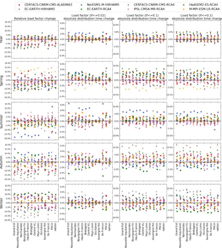
In the long-term future, climate change may impact the wind power potential and its intermittency, which could consequently influence the electricity system operation and planning. In this section, we investigate the impact of climate change on the French wind power production by comparing the load factor during one future period (2046–2055) and one historical period (2006–2015) using 8 EURO-CORDEX simulations under two different emission scenarios (RCP4.5 and RCP8.5). The choice of these two periods is driven by the long-term electricity system tran-sition studies projected on 2050, while 2006–2015 is representative of the present climate. We analyze the long-term change at a regional level and also at the aggregated national scale. The onshore wind distribution is assumed to be the same as that at the end of 2019. The offshore wind power is assumed to be distributed equally over the 11 sites discussed above. We first analyze the changes in annual and seasonal mean and distribution, and then focus on the changes in intermittency.
Fig. 12. Annual-average Load factor for various sites where offshore wind
farms are planned in France, for the improvement due to advanced hub-height effect in 2030 (green bar) and 2050 (red bar), compared to current status in 2020 (blue), as derived from EPPCF model using ERA5 reanalysis wind speed data for regional and national offshore wind.
Fig. 13. Same as Fig. 5 but for the Offshore wind projects. The data used is based on simulation result in using EPPCF method applying ERA5 wind speed data from