In situ terminal settling velocity measurements at Stromboli volcano: Input from physical characterization of ash

HAL Id: hal-02057537

https://hal.uca.fr/hal-02057537

Submitted on 24 Jan 2020

HAL is a multi-disciplinary open access

archive for the deposit and dissemination of sci-entific research documents, whether they are pub-lished or not. The documents may come from teaching and research institutions in France or abroad, or from public or private research centers.

L’archive ouverte pluridisciplinaire HAL, est destinée au dépôt et à la diffusion de documents scientifiques de niveau recherche, publiés ou non, émanant des établissements d’enseignement et de recherche français ou étrangers, des laboratoires publics ou privés.

In situ terminal settling velocity measurements at

Stromboli volcano: Input from physical characterization

of ash

V. Freret-Lorgeril, F. Donnadieu, Julia Eychenne, C. Soriaux, T. Latchimy

To cite this version:

V. Freret-Lorgeril, F. Donnadieu, Julia Eychenne, C. Soriaux, T. Latchimy. In situ ter-minal settling velocity measurements at Stromboli volcano: Input from physical characteriza-tion of ash. Journal of Volcanology and Geothermal Research, Elsevier, 2019, 374, pp.62-79. �10.1016/j.jvolgeores.2019.02.005�. �hal-02057537�

In situ terminal settling velocity measurements at Stromboli

volcano: Input from physical characterization of ash

V. Freret-Lorgeril1_{, F. Donnadieu}1,2_{, J. Eychenne}1_{, C. Soriaux}1_{, T. Latchimy}2_.

3

1_{Université Clermont Auvergne, CNRS, IRD, OPGC, Laboratoire Magmas et Volcans,}

F-4

63000 Clermont-Ferrand, France 5

2_{CNRS, UMS 833, OPGC, Aubière, France}

6

Corresponding author: valentin.freretlo@gmail.com 7

8

ABSTRACT

9

Ash particle terminal settling velocity is an important parameter to measure in order to 10

constrain the internal dynamics and dispersion of volcanic ash plumes and clouds that emplace 11

ash fall deposits from which source eruption conditions are often inferred. Whereas the total 12

Particle Size Distribution (PSD) is the main parameter to constrain terminal velocities, many 13

studies have empirically highlighted the need to consider shape descriptors such as the 14

sphericity to refine ash settling velocity as a function of size. During radar remote sensing 15

measurements of weak volcanic plumes erupted from Stromboli volcano in 2015, an optical 16

disdrometer was used to measure the size and settling velocities of falling ash particles over 17

time, while six ash fallout samples were collected at different distances from the vent. We focus 18

on the implications of the physical parameters of ash for settling velocity measurements and 19

modeling. Two-dimensional sizes and shapes are automatically characterized for a large 20

number of ash particles using an optical morpho-grainsizer MORPHOLOGI G3. Manually 21

sieved ash samples show sorted, relatively coarse PSDs spanning a few microns to 2000 μm 22

with modal values between 180-355 μm. Although negligible in mass, a population of fine 23

particles below 100 μm form a distinct PSD with a mode around 5-20 μm. All size distributions 24

are offset compared to the indicated sieve limits. Accordingly, we use the diagonal of the upper 25

mesh sizes as the upper sieve limit. Morphologically, particles show decreasing average form 26

factors with increasing circle-equivalent diameter, the latter being equal to 0.92 times the 27

average size between the length and intermediate axes of ash particles. Average particle 28

densities measured by water pycnometry are 2755 ± 50 kg m-3 and increase slightly from 2645 29

to 2811 kg m-3 with decreasing particle size. The measured settling velocities under laboratory 30

conditions with no wind, < 3.6 m s-1, are in agreement with the field velocities expected for 31

particles with sizes < 460 μm. The Ganser (1993) empirical model for particle settling velocity 32

is the most consistent with our disdrometer settling velocity results. Converting disdrometer 33

detected size into circle equivalent diameter shows similar PSDs between disdrometer 34

measurements and G3 analyses. This validates volcanological applications of the disdrometer 35

to monitor volcanic ash sizes and settling velocities in real-time with ideal field conditions. We 36

discuss ideal conditions and the measurement limitations. In addition to providing 37

sedimentation rates in-situ, calculated reflectivities can be compared with radar reflectivity 38

measurements inside ash plumes to infer first-order ash plume concentrations. Detailed PSDs 39

and shape parameters may be used to further refine radar-derived mass loading retrievals of the 40

ash plumes. 41

Highlights:

42

• An optical disdrometer is used to measure ash sizes and settling velocities at Stromboli. 43

• Collected ash samples show sorted and coarse particle size distributions. 44

• Ash particles density and sphericity slightly decrease with augmenting size. 45

• Ganser’s law (1993) best fits disdrometer field measurements of settling velocities. 46

• Volcanological applications of disdrometers to monitor ash fallout are validated. 47

48

Keywords: Terminal Settling Velocity; Ash fallout; Particle size; Morphology;

49

Disdrometer; Stromboli.

50 51

1. Introduction

Constraining volcanic ash plume dynamics, dispersion and fallout processes is of 53

paramount importance for the mitigation of related impacts, such as those on infrastructure, 54

transportation networks, human health (Baxter, 1999; Wilson et al., 2009; Wilson et al., 2012). 55

The terminal settling velocity (VT) of particles transported in volcanic ash plumes influences

56

plume dispersal in the atmosphere, controls the sedimentation pattern in space and time, and in 57

turn, the formation of ash deposits (Beckett et al., 2015; Bagheri & Bonadonna, 2016a). VT is

58

used to estimate ash mass deposition rates (Pfeiffer et al., 2005; Beckett et al., 2015) and it 59

mainly depends on the total grain size distribution (TGSD), and the density and the shape of 60

ash particles. Retrieving the TGSD in real-time is currently impossible for operational purpose 61

owing to the lack of direct measurements of the in situ Particle Size Distribution (PSD; e.g., 62

inside the plume). It is generally obtained from post-eruption analyses of ash deposits 63

(Andronico et al., 2014) or from a multi-sensor strategy (Bonadonna et al., 2011; Corradini et 64

al., 2016) comprising, for instance, satellite images (Prata, 1989; Prata & Grant, 2001; Prata & 65

Bernardo, 2009) and radar remote sensing (Marzano et al., 2006a, 2006b), coupled to ground 66

sampling. Meteorological optical disdrometers, although originally designed for hydrometeors, 67

can be used to record volcanic ash fallout, and provide particle number density, settling 68

velocities and sizes in near real-time at a single location. Disdrometer measurements can be 69

used to calibrate dispersion model outputs, as well as radar observations from an empirical law 70

relating derived radar reflectivity factors and associated particle mass concentrations. First-71

order estimates of their mass loading parameters, of primary importance for hazard evaluation, 72

can then be made by comparing the calculated reflectivities to radar measurements inside ash 73

plumes (Maki et al., 2016). 74

Volcanic Ash Transport and Dispersion (VATD) models require equations relating VT

75

to particle size distribution in order to make accurate forecasts of ash dispersion and deposition. 76

As VT also depends on particle shape parameters and densities, these need to be characterized

77

as a function of sizes. Ash particles are highly heterogeneous in shape and size due to a variety 78

of fragmentation processes (Cashman & Rust, 2016), leading to the development of empirical 79

laws describing the aerodynamic drag of the particles, from which terminal velocity depends. 80

Initially this was done for spherical grains (Gunn & Kinzer, 1947; Wilson & Huang, 1979 and 81

references therein) and then for non-spherical particle shapes based on laboratory experiments 82

(Kunii & Levenspiel, 1969; Ganser, 1993; Chien, 1994; Dellino et al., 2005; Coltelli et al., 83

2008; Dioguardi & Mele, 2015; Bagheri & Bonadonna, 2016b; Del Bello et al. 2017; Dioguardi 84

et al., 2017). Such studies have revealed the need to consider the morphological aspects of ash 85

particles to refine VT estimates, in addition to the total grain size distribution.

86

A geophysical measurement campaign at Stromboli volcano was carried out between 87

the 23rd of September and the 4th of October 2015 to characterize the mass load of ash plumes 88

and their dynamics using radars at different wavelengths, including a millimeter-wave radar for 89

ash tracking (Donnadieu et al., 2016). In addition, falling ash particles were measured in-situ 90

and in real-time using an optical disdrometer and samples from ground tarps, in order to 91

constrain the PSD. The PSD is required to quantify the mass load parameters of the plume from 92

the radar reflectivity measurements. 93

In this paper, we present a physical characterization of ash particles from Strombolian 94

weak plumes using ash samples collected from ground tarps and near-ground disdrometer 95

measurements of the falling ash. Section 2 focuses on the instruments and methodologies 96

utilized to characterize ash samples and these results are presented in section 3. In section 4 we 97

present VT measurements of ash particles obtained in the field and under laboratory conditions

98

and compare them to existing empirical models. We discuss the results and limitations and then 99

give conclusive remarks of this study in section 5 and 6, respectively. 100

2. Materials and methods

2.1 Ash sampling in the field

102

Ash samples from ash-laden plumes of Stromboli volcano were collected on the ground 103

from a 0.4 m2 tarp (0.45 m × 0.9 m) and a collector (0.6 m × 0.6 m) during a Doppler radar 104

measurement campaign between the 23rd September and the 4th October 2015 (Donnadieu et 105

al., 2016). During this period, Stromboli eruptive activity was weak, producing type 2a and/or 106

2b eruptions (Patrick et al., 2007), which are characterized by the emission of ash plumes rising 107

200 to 400 m high above the active vents, and drifted towards the North to the North-East with 108

prevailing winds. Six ash samples from different ash fallout events were collected on a ground 109

tarp at different locations and distances from the area of the craters: (i) two on the NE flank 110

(Roccete) 500 to 600 m from the summit vents (white cross in Figure 1), (ii) three near Pizzo 111

Sopra la Fossa, ~320-330 m northeast of the SW crater (blue cross in Figure 1), next to the 112

optical disdrometer (white square in Figure 1), and (iii) one in a collector at Punta Labronzo 113

~2 km to the North (green cross in Figure 1). Details on ash sample collection dates and 114

locations are summarized in Table 1. 115

Table 1: Date and locations of the six collected ash samples.

116 Date (mm/dd/yyyy) Eruption time UTC (HH:MM)

location Sample names GPS point (UTM)

Collected mass (g)

09/25/2015 16:36 near Pizzo

Sopra la Fossa 1636_summit

33 S 0518663 UTM 4293821 0.642 10/02/2015 12:46 NE flank (Roccete) 1246_roc 33 S 0518774 UTM 4294327 4.971 10/02/2015 15:30 Punta Labronzo 1530PL 33 S 0518720 UTM 4295743 0.259 10/02/2015 15:50 near Pizzo

Sopra la Fossa 1550_summit

33 S 0518663 UTM 4293821 0.068 10/03/2015 10:42-12:52 NE flank (Roccete) 1042-1252_roc 33 S 0518774 UTM 4294327 6.801 10/03/2015 16:01 near Pizzo

Sopra la Fossa 1601_summit

33 S 0518663

UTM 4293821 25.230 117

119

Figure 1: Map of Stromboli Island. The Optical disdrometer was set up next to Pizzo Sopra la Fossa at

120

900 m a.s.l. (white square), 320 m and 330 m away from the NE (white triangle) and the SW crater (red

121

triangle), respectively. Ash samples were collected at Pizzo Sopra la Fossa next to the disdrometer (blue

122

cross), on the NE flank (Roccete) 500-670 m NE from the vents (white cross) and at Punta Labronzo

123

(1530PL sample, green cross) about 2 km North from the vents.

124

2.2 Grain-size and morphological analyses

125

The samples were manually sieved twice to determine their PSDs at 1/2 Φ and 1/4 Φ 126

intervals. The mass of each fraction was measured with a 10-4 g accuracy weighing scale. The 127

relation between Φ scale and circle equivalent diameters (D) is given by Φ = - log2(D (mm)).

128

In total, less than 0.5% of the mass of ash collected was lost during the 1/2 Φ mechanical 129

sieving. We calculated the sorting coefficient S0 from Folk & Ward (1957):

130 0 84 16 95 5 4 6.6 S =  −  + −  , (1) 131

with Φ84, Φ16, Φ95 and Φ5 being the Φ values corresponding to the 84th_{, the 16}th_{, the 95}th _and

132

the 5th _{percentiles, respectively, of the calculated PSD. The lower the S}

0, the more sorted the

133

PSD. 134

To study the size and shapes of ash particles, we use the MORPHOLOGI G3TM 135

automated optical analyzer (named G3 is this study) designed by Malvern InstrumentsTM_.

136

Particles from a given sieve are placed on a glass plate and illuminated from below (diascopic 137

illumination). The G3’s microscope measures the 2-D projected areas and shapes of a sample 138

of particles, allowing an automatic analysis of morphological parameters such as the size and 139

2-D shape parameters. We used a × 5 magnification leading to an image resolution of 3.3 140

pixel/µm2 (i.e. less than 0.5 µm of minimum resolution). Typically, tens of particles of size 1 141

Φ up to 18000 particles of size < 4 Φ can be processed in 35 minutes (fast and routine analyzes, 142

Leibrandt & Le Pennec, 2015). In order to reduce the size range of the individual particles 143

analyzed while keeping them optically focused, the half- Φ fractions were sieved at a 1/4 Φ. 144

Obtained sieving results are presented in Appendix A. 145

We measure the following size parameters: (i) the longest axis (L) and (ii) intermediate 146

axis (I) in the 2-D plane orthogonal to the light direction; (iii) the circle-equivalent diameter 147

DCE = 2 × (Ap/π)1/2 measured from the particle section area Ap; and (iv) the sphere-equivalent

148

volume calculated with diameter DCE. Due to the 2-D imaging inherent to the methodology, we

149

assume that particles always show the maximum projection area (Bagheri & Bonadonna, 2016) 150

and, hence, their short (S) axes are always oriented orthogonal to the image plan, i.e. S ≤ I. 151

From the measurements of L, I and Ap, the following morphological parameters are

152

defined: (i) the Elongation e = I/L (Bagheri & Bonadonna, 2016b); (ii) the Convexity Cv =

153

PCH/Pp, corresponding to the textural roundness of the particles with perimeter Pp (Liu et al.,

154

2015), and PCH being the convex hull perimeter (i.e. the smallest convex polygon containing all

155

pixels of the analyzed particle); (iii) the solidity Sd= Ap/ACH (Cioni et al., 2014), indicative of

156

the high wavelength (i.e., morphological) roughness of the particles (Cioni et al., 2014; Liu et 157

al., 2015b) with ACH being the convex hull area; and (iv) the sphericity φ = 4πAp/Pp2 as an

158

indicator of the roughness and the shape of the particles (Riley et al., 2003). The sphericity φ is 159

equal to the square of the circularity Cc (i.e. equal to 2(πAp)1/2/Pp) defined by Leibrandt & Le

160

Pennec (2015). According to Liu et al. (2015a), the shape parameters associated to the convex 161

hull, such as Sd and Cv, characterize the roughness of particles independently of their form.

These parameters range from 0 to 1 (e.g., a perfect sphere has a value of 1) and are all described 163

in Leibrandt & Le Pennec (2015), Liu et al. (2015a, 2015b) and Riley et al. (2003). 164

A complete PSD from G3 analyses, comprising all analyzed 1/4 Φ sieved fractions, is 165

estimated by combining (i) the measured mass fractions from 1/4 Φ sieving with (ii) the sphere-166

equivalent volume (VSE) of particles measured by the G3 for each analyzed fraction:

167

(

)





where subscript i denotes the size bin containing individual particles analyzed by the G3 having 169

a DCE diameter within the upper and lower bounds of the bin, whereas subscript j stands for the

170

sieve size fraction from manual sieving. Each bin i has a 5 µm resolution and the uncertainty 171

associated with the G3 image resolution is thus considered as negligible. miwt% is the weight

172

fraction of particles in the ith bin size, and mjwt% is the mass percentage of the analyzed sieve

173

fraction j of the total sample mass. The ratio i j_, /

(

)

E i

S j

V



ratio of particles belonging to the ith bin size with respect to all particles from a sieved fraction 175

j. We use the sphere-equivalent volume derived from the G3, rather than the number of 176

particles, to minimize the error propagation in the mass calculation due to the large increase in 177

particle number with decreasing size. 178

2.3 Ash density measurements

179

The average densities of ash particles of 1/4 Φ sieved fractions of the two samples with 180

the largest mass (1601_summit and 1246_roc) are measured by water pycnometry (Eychenne 181

& Le Pennec, 2012). This method allows the estimation of ash particle density by volume 182

difference between a 9.5 × 10-6 m3 boro-silicate pycnometer filled with distilled and degassed 183

water and then filled with water and a known mass of ash sample. 184

The density of particles is given by: 185 1 2 i w i w w m m m   = − , (3) 186

with ρi the density of the ith ash size class in kg.m-3, ρw the density taken to be 1000 kg m-3, mi

187

the mass of ash incorporated into the pycnometer (0.4 to 2 g), mw1 the mass of water required

188

to fill the reference pycnometer volume and mw2 the mass of water required to fill the

189

pycnometer once the ash sample has been added. 190

By using water pycnometry, we measure the average particle density of a given sieved 191

fraction. For particles between 125 μm and 700 μm, we assume that water surface tension can 192

be considered as sufficiently strong to avoid vesicle and asperity filling. For this hypothesis to 193

be verified, the particles are dried in an oven before being incorporated into the water (Eychenne 194

& Le Pennec, 2012). Thus, the measured densities correspond to the apparent densities of the 195

particles, which represents their mass divided by their solid volume and the volume linked to 196

their porosity. 197

2.4 The optical disdrometer and particle settling experiments

198

The optical disdrometer Parsivel2, designed by OTT, uses a 780 nm wavelength laser 199

beam emitted from a transmitter to a receiver, which converts the transmitted laser light into a 200

voltage signal. Described in Löffler-Mang & Jürg (2000) and Tokay et al. (2014), the 201

disdrometer measures the settling velocities and sizes of particles when as they pass through 202

the laser sheet. The laser obscuration time is used to estimate the settling velocities. The longer 203

a particle takes to cross the beam, the lower the settling velocity. Then, the amplitude of the 204

laser light extinction is used to calculate the size of the particles. By measuring the number of 205

falling particles and their settling velocity class values (Appendix B), the disdrometer 206

calculates the number density of particles crossing the beam as: 207 ( ) d i i i i i n N D v A t D =  , (4) 208

with Ni(Di) the particle number density (mm-1 m-3) of the ith disdrometer size class, ni the

209

number of detected particles with measured settling velocity vi (m s-1), A the laser sheet area

210

(54 × 10-4 m2), Δt the sampling interval (10 s) and dDi the size range (mm) of the disdrometer

211

ith size class. The disdrometer measures settling velocities between 0.05 and 20.8 m s-1 212

distributed among 32 classes (Classes 1 to 22 are displayed in Appendix B) and detects 213

particles with diameter from 250 µm to 26 × 103 µm. 214

We performed in-situ measurements of falling ash during the field campaign at 215

Stromboli. The disdrometer was set up about 80 cm above the ground close to Pizzo Sopra La 216

Fossa (Figure 1), 320-330 m northeast of the SW crater. The disdrometer recorded the ash 217

fallout events from weak Strombolian plumes that produced the two ash samples collected from 218

ground tarps next to the disdrometer (1601_summit) and lower down the NE flank (1246_roc). 219

In order to establish the ash fallout detection limits of the disdrometer and to estimate 220

the influence of the wind on particle settling velocities in the field, disdrometer retrievals are 221

tested under laboratory conditions of no horizontal nor vertical wind. Sieved ash particles from 222

the 1601_summit sample are dropped from heights between 3 m and 11 m above the 223

disdrometer laser sheet in order to verify that terminal settling velocities were reached for each 224

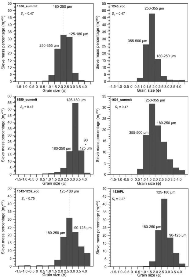
sieved size fraction. 225

2.5 Terminal settling velocity models

226

The terminal settling velocity depends on the size, the shape and the density of falling 227

particles that affect their drag forces and hence the flow regime adopted by the ambient carrier 228

fluid. For individual particle settling, VT is defined by the following equation (Wilson & Huang,

229

1979; Woods & Bursik, 1991; Sparks et al., 1997): 230 4 ( ) 3 a T CE a D g V D C    − = , (5) 231

where VT is the terminal settling velocity of the particle (m s-1), DCE is the circle-equivalent

232

diameter corresponding to the diameter of a circle (applicable to a sphere) with area measured 233

by the G3 for each particle, g is the gravitational acceleration (m s-2), ρ and ρa are the particle

234

and air densities, respectively, in kg m-3. Here, ρa is equal to 1.2 kg m-3 at a temperature of 15

235

°C at sea level (similar to laboratory conditions) and equals to 1.12 kg m-3 at 900 m a.s.l. (similar 236

to field conditions). Finally, CD is the drag coefficient and depends on the shapes of the settling

237

particles and the Reynolds number Re, which describes the flow regime in which particles fall: 238 T a V D Re   = , (6) 239

where VT corresponds to the settling velocity of a particle within a non-moving ambient fluid

240

(i.e. the air in this case) with a viscosity μ (Pa s) equals to 1.85 × 10-5 _{Pa s at a temperature of}

241

15 °C at sea level (similar to laboratory conditions) and equals to 1.786 × 10-5 _{Pa at 900 m a.s.l.}

242

(similar to field conditions). 243

To verify that ash particles were falling at their VT, we compared the disdrometer

244

measurements with empirical VT laws that are based on the following assumptions.

245

First, for particle Reynolds Number between 0.4 and 500 at an altitude of 5 km above 246

sea level (a.s.l.) and assuming spherical particle diameters less than 1500 µm, VT of a particle

247

can be expressed as (Kunii & Levenspiel, 1969; Bonadonna et al., 1998; Coltelli et al., 2008): 248 1 2 2 ₃ 4 255 T a g V D     =     , (7) 249

Then, we compare our results with the models of Ganser (1993) and Bagheri & 250

Bonadonna (2016b) based on Equation 5, which account for non-spherical particle shapes. In 251

such a case, the drag equations are derived from empirical analyses of particle settling velocities 252

and are not related to the same particle shape parameters. 253

In Ganser (1993), CD is determined as follows:

254

(

)

K1 and K2 being the Stokes' shape factor and the Newton's shape factor, respectively:

256 1 1 2 1 1 2 3 3 K  − −   =_ + _   , (9) 257 ( )0.5743 1.8148 log 2 10 K = −  , (10) 258

where φ is the G3-derived sphericity (Riley et al., 2003) of particles considered as isometric (I 259

=S) and is the best shape parameter to be used in the Ganser model (Alfano et al., 2011). 260

In Bagheri & Bonadonna (2016b), CD is calculated as: 261 2 3 24 0.46 1 0.125 1 5330 S N D S N S k k C Re Re k k Re k    _{ }        = _ + _{   }+ _     ₊              , (11) 262

with kS and kN, being shape factors equal to:

263 k (F1/ 3 F 1/ 3) / 2 S s s − = + , (12) 264 where 1.3 3 CE S D F f e L I S   = _{ }   and 3 2 CE N D F f e L I S   = _{ }   265 and 266

( )

where2 =0.45 10 / exp(2.5log+ ( / a)+30) and 2 = −1 37 / exp(3log( / a)+100)

268

These shape factors depend on 3-D ash particle axes such as L, I, S and also the 269

elongation (I/L) and flatness (S/I). 270

Because CD, Re and VT are dependent on each other, we use an iterative approach to

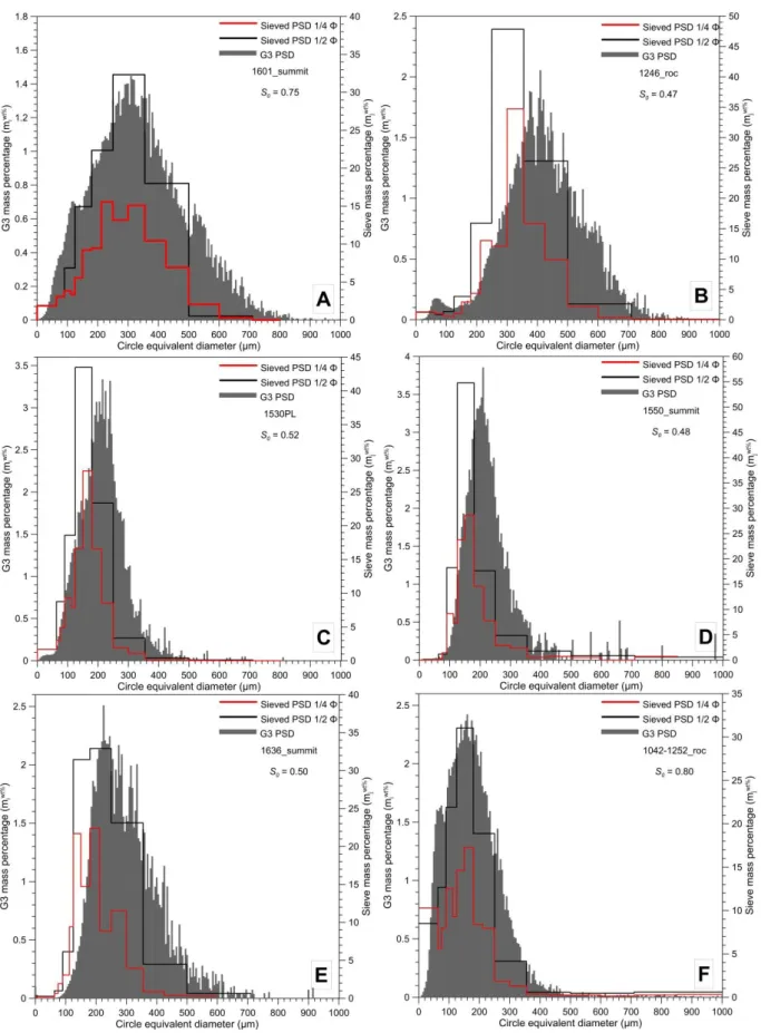
271

determine the settling velocities with both aforementioned models. We initialize VT using the

272

Stokes law, where VTStokes = (g DCE2 (ρ- ρa))/18μ, and then iteratively calculate Re, CD, and VT

273

(Equation 5). The iterations are stopped when the velocity difference is less than 10-8. 274

Finally, we calculate VT using the Dellino et al. (2005) relationship:

275

(

)

(

)



  





where ψ is a shape factor defined as the ratio between the particle sphericity (Riley et al., 2003) 277

and 1/Cc. Thus, the combination of Equation 5 and the drag coefficient of spherical particles

278

leads to the equation of Dellino et al. (2005), which does not depend on CD and Re. Equation

279

14 is only valid for Reynolds number > 60-100 (Dioguardi et al., 2018).

Ash morphological parameters are required in order to compare models of VT for

non-281

spherical particles to ash settling velocities measured in the field or under laboratory conditions. 282

These parameters are characterized in the following section for Strombolian ash. 283

3 Ash characteristics

3.1 Particle size distribution by mechanical sieving and morpho-grainsizer

285

Here we present sieving results obtained for the six ash samples. Values are available in 286

Appendix A. The PSD from 1/2 Φ sieving for the proximal samples collected on the summit

287

have modal values ranging from 125-180 μm (1550_summit) to 250-355 μm (1601_summit) 288

(Figure 2). The same range of PSD modes is observed for the proximal samples collected lower 289

down on the East flank at Roccete (1042-1252_roc and 1246_roc). The 1530PL sample 290

collected 2 km to the North of the summit vent at Punta Labronzo shows a mode at 125-180 291

μm. Particle sizes range from < 63 μm to 1400 µm in 1246_roc and from < 63 μm to 2000 µm 292

in 1601_summit (Figure 2). Therefore, there is no obvious correlation between sample location 293

and PSD, an observation also made by Lautze et al. (2013) on ash samples from type 2 eruptions 294

at Stromboli in 2009. Sorting coefficients S0 of 0.27-0.47 indicate sorted PSDs for all ash

295

samples from a single ash plume (Figure 2). The higher sorting coefficient S0 of 0.75 for the

296

1042-1252_roc sample is due to the collection of a 2-hour long succession of fallout events 297

with potentially variable PSDs, the sum of which leads to a less sorted PSD. We cannot exclude 298

some dust contamination from this sample. 299

Following the 1/4  sieving, the particle number frequency histogram of each sieved 300

fraction is calculated from the G3 analyses. As observed by Leibrandt & Le Pennec, 2015, 301

PSDs from the sieve fractions show a large offset toward DCE values larger than the sieve mesh

302

sizes. In particular, the modal DCE can lay well beyond the sieve mesh limits as shown for the

303

1601_summit sample (fractions < 63 μm to 425-500 μm; Figure 3). For example, the 250-300 304

μm sieve fraction (red PSD in Figure 3) actually ranges between 248-551.78 μm in DCE, with

305

a mode at 350 μm, leading to 95.1% of the PSD lying above the upper sieve limit. 306

307

Figure 2: 1/2  Particle size distributions determined by manual sieving for the six ash samples of

308

Table 1. S0 is the Folk & Ward (1957) sorting coefficient. Lower S0 indicates better sorting. 309

311

Figure 3: Individual particle number frequency histograms retrieved from the G3 analyses of 1/4

312

 sieved fractions from the 1601_summit ash sample. Shaded red areas highlight the sieve intervals in

313

circle-equivalent diameter and the percentage of the PSD larger than the upper sieve mesh is displayed

314

in red. The vertical purple dashed lines indicate the diagonal dimension of the sieve upper mesh size, a

315

better fit to the true PSD upper bound, as shown by the small residual percentage of the PSD (in black)

316

larger than the diagonal of the sieve upper mesh. The intervals of the corrected sieve mesh sizes (down

317

mesh size to diagonal of the upper mesh size) are indicated in color above each histogram.

318

The number proportion of the PSD lying above the upper sieve limit increases with sieve 319

mesh size, with a minimum value of 26.2% for the < 63 μm fraction and up to 96.2% for the 320

425-500 μm fraction. This discrepancy is explained by the fact that sieve mesh sizes (side 321

dimension of the squared mesh) are given for supposedly spherical particles, whereas ash 322

particles are non-spherical and often depart significantly from a spherical shape. Therefore, 323

many particles with their largest and intermediate axes higher than the mesh size can be found 324

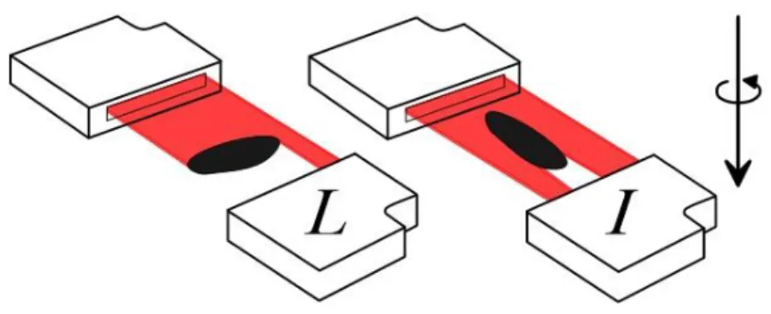
in the sieved fraction depending on their orientation while passing through the mesh. The length 325

of the squared mesh diagonal, as opposed to the mesh size, represents the true sieve upper limit 326

when dealing with non-spherical particles, as shown by the small residual percentages of the 327

PSD (1-6%) above the upper mesh diagonal length. Consequently, we use the lower mesh size 328

and the diagonal length of the upper mesh, i.e. the upper mesh side length multiplied by 2 329

(vertical purple dashed line in Figure 3), to characterize the circle-equivalent diameter 330

distributions of ash particles. These bounds of DCE contain more than 94% of the ash particles

331

in each fraction and are thus representative. In this new reference frame, for example, the 250-332

300 μm sieve fraction (i.e. Φ=2) has DCE lower and upper limits of 250 and 424.3 μm.

333

334

Figure 4: Comparison of mass- and number-based PSD in the 125-254.6 μm sieve fraction from the

335

1601_summit ash sample. The right axis represents the number frequency measured by G3 (blue

336

histogram). The left axis represents the particle mass percentage mi% (orange bars) using sphere-337

equivalent volumes measured by the G3.

338

Every sieved fraction of the six ash samples, when analyzed in number frequency, shows 339

a distinct population of very fine ash particles with a relatively constant modal value between 340

5-20 μm. For example, in the 125-254.6 μm fraction of the 1601_summit sample (blue 341

histogram in Figure 4), the secondary PSD of fine ash represents 73% of the total sieved 342

fraction PSD in terms of particle number frequency (blue histogram in Figure 4), whereas these 343

very fine particles represent only 3% of the whole PSD in mass or volume percentage. Likewise, 344

in the other sieve fractions, the population of very fine ash appears as a decoupled PSD with a 345

high contribution to the particle number frequency, but negligible in terms of mass or volume. 346

Finally, because DCE distributions among successive sieve fractions exhibit a dramatic

347

overlap (Figure 3), we calculate mass percentages (Equation 2) over the whole PSD in 5 μm 348

bins by weighting the high resolution sphere-equivalent volume from the G3 analyses with the 349

mass percentage of each sieved fraction at 1/4 Φ. This calculation leads to high resolution (5 350

μm) mass percentage PSDs for the six ash samples (Figure 5). They show a unimodal 351

distribution whereas the 1/4 Φ sieves displaytwo close maxima, the latter due to splitting of a 352

unique mode at the bin transition (250 μm) into adjacent bins in Figures 5A and 5F. For the 353

1601_summit and the 1042-1252_roc samples (Figure 5A and Figure 5F), the PSD obtained 354

from the 1/2 Φ sieving broadly matches the corrected high resolution PSD in terms of modal 355

value, whereas the 1/4 Φ PSDs tend to show a mode lower than that of the corrected PSD. 356

Unlike the 1601_summit and 1042-1252_roc calculated PSD, the other calculated PSDs are 357

well sorted (0.47-0.52). 358

The aforementioned artificial offset of the sieving PSDs toward smaller DCE is more

359

obvious in the other ash samples (Figures 5B, 5C, 5D and 5E), emphasizing the significant 360

bias on resulting PSD introduced by sieving non-spherical particles. Indeed, whereas spherical 361

particles would be blocked by a sieve squared mesh having its side length corresponding to 362

their diameter, coarser particles with some degree of elongation can cross the squared mesh 363

along its diagonal (side length times 2) and appear in lower (smaller mesh-sized) sieves. As 364

sieve mesh size intervals increase with diameter (i.e. decreasing Φ), the shift in diameter 365

increases for coarser particles. Therefore, the sieving-derived PSDs agree more closely with 366

high resolution PSDs derived from optical measurements for finer particles. 367

368 369

370

Figure 5: Comparison of the PSDs calculated from G3 analyses with the PSDs inferred from manual

371

sieving (1/4 Φ, red step line; 1/2 Φ, black step line) for the six ash samples 1601_summit (A), 1246_roc

372

(B), 1530PL (C), 1550_summit (D), 1636_summit (E), and 1042-1252_roc (F).

373 374

3.2 Ash densities

375

To constrain VT, we use water pycnometry to measure the density of ash samples from

376

the fallout detected by the optical disdrometer. Samples 1246_roc and 1601_summit have 377

similar density trends (Figure 6). The average particle density of all measurements from the 378

two summit samples is equal to 2755 ± 58 kg m-3. The density trend beyond Φ  2.5 is uncertain 379

because the measurement’s accuracy is lower for fine particles and small sample mass, as seen 380

from the increased spread of the 1601_summit measurements for Φ  2.5. For this reason, we 381

mixed the 3.5 to 2.5 Φ fractions of the 1246_roc sample to calculate a more representative 382

average density of 2811 ± 55 kg m-3. In both samples, average densities slightly decrease with 383

increasing diameter from Φ=2.5 to Φ=1 (i.e. 180-500 µm) from a maximum value of 2811 ± 384

55 kg m-3 to 2645 ± 35 kg m-3. Over a particle size distribution, tephra densities typically form 385

a sigmoidal trend that was previously described for andesitic, dacitic and rhyolitic ash 386

(Eychenne & Le Pennec, 2012; Cashman & Rust, 2016). This sigmoidal trend is apparent for 387

Φ ≤ 0.5 (i.e. DCE  710 µm) and the slight density decrease with increasing diameter might

388

represent the beginning of a sigmoidal trend in density variation. 389

390

Figure 6: Ash densities determined by water pycnometry for the two samples 1601_summit (grey dots)

391

and 1246_roc (red diamonds) as a function of the 1/4 Φ fractions. Dashed lines correspond to the

392

average density of each grain size class.

393 394

3.3 Particle shapes

395

A comparison between Sd and Cv of the modal PSD classes of the six distinct ash

396

samples (Figures 2 and 5) shows homogeneous average distributions of textural and 397

morphological roughness among all samples (Figure 7A and Table 2). This observation is 398

similar to morphometric analyses done by Lautze et al. (2011, 2013) at Stromboli showing no 399

obvious relationship between particle shapes and the relatively short distance travelled from the 400

source vent. In all samples, the average values of Sd and Cv are similar (Table 2) except for the

401

1042-1252_roc sample, which records several fallout events over a longer collection time, as 402

opposed to the other samples, and is possibly contaminated by wind-drifted dust. Particles show 403

high average solidity and convexity of 0.954 and 0.943, respectively (snapshot in Figure 7A). 404

Though rare, irregular shaped particles can be found in several samples. Such particles, 405

characterized by the lowest values of Cv and Sd (i.e. 0.747 in sample 1530PL and 0.545 in

406

sample 1246_roc), are displayed in Figure 7A. In total, and among all the samples, more than 407

90% of the analyzed particles show Cv and Sd values higher than 0.9, which characterize dense

408

ash fragments (Liu et al., 2015b). 409

Among the 6 samples, there is no clear systematic trend in sphericity as a function of 410

particle size (Figure 7B). Sieved fraction average φ are within a narrow range between 0.7 and 411

0.92 (< 63 to 750 μm fractions) and decrease under 0.7 to minimum values of 0.5 in the 1530PL 412

sample. Nevertheless, with respect to the standard deviation of sphericity in the 1601_summit 413

sample, there is no significant variation of φ with DCE up to 750 μm, beyond which values

414

decrease slightly. 415

Table 2: Average Convexity Cv, Solidity Sd and Sphericity φ values of the modal sieved fractions (1/4 416

Φ) of the PSD for the six ash fallout samples.

417 Sample names Corrected Mesh (μm) mean Cv Standard deviatio n Mean Sd Standard deviation mean φ Standard deviation 1246_roc 300-502 0.956 ± 0.020 0.947 ± 0.027 0.770 ± 0.067 1601_summit 300-502 0.945 ± 0.020 0.947 ± 0.026 0.765 ± 0.068 1530PL 150-254.6 0.955 ± 0.022 0.943 ± 0.031 0.762 ± 0.076 1550_summit 150-254.6 0.957 ± 0.023 0.939 ± 0.034 0.759 ± 0.081 1636_summit 180-299.8 0.955 ± 0.024 0.938 ± 0.034 0.757 ± 0.081 1042-1252_roc 150-254.6 0.921 ± 0.032 0.927 ± 0.033 0.707 ± 0.081

418

Figure 7: A) Clustergram of Convexity (Cv) as a function of the Solidity (Sd) of particles pertaining to 419

the modal sieved fraction of the PSD for the 6 ash fallout samples. Average values of each population

420

and their standard deviations are indicated in red bars and symbols. B) Average Sphericity (φ) of the

421

sieved fractions as a function of their average circle-equivalent diameter (DCE). C) Average Circle-422

equivalent diameter (DCE) as a function of the average Length (L) and average Width (I). D) Average 423

elongation (I/L) as a function of sieved fractions average DCE. Errors bars (standard deviation) are 424

shown in grey for the 1601_summit average values.

425

The observation of particle shapes is essential to understand the measurements of the 426

optical disdrometer in terms of VT and sizes. Here, we assume that detected ash particles tend

427

to fall perpendicularly to the plane defined by their maximum (L) and intermediate (I) axes 428

(Bagheri & Bonadonna, 2016). Therefore, the disdrometer should measure sizes ranging 429

between L and I, and an average value statistically approaching (I+L)/2 if a random orientation 430

of the particle L (or I) axis in the beam plane is assumed (see Figure 8). Taking into account 431

the linear relationships of axes dimensions with particle DCE found in Figure IV.7C for all

432

analyzed ash particles at Stromboli, DCE can be equated on average to 0.92 (I+L)/2 with a high

433

correlation (R2 _{= 0.999). This relationship is used thereafter to find the circle-equivalent}

434

dimension of the disdrometer sized classes recording non-spherical ash particles. Hence, the 435

lower detection limit of the disdrometer of 250 μm corresponds to 230 μm in circle-equivalent 436

diameter. 437

438

Figure 8: Schematic representation of particle orientation when crossing the disdrometer laser 439

beam. Assuming random rotating motion and no tumbling, particles may present a length, 440

which is assumed to be equal to (I+L)/2. 441

With increasing DCE, the I/L ratio (i.e. the particle elongation of Bagheri & Bonadonna,

442

2016b) increases non-linearly from 0.66 for DCE < 63 μm to 0.83 for DCE > 710-1414 μm

443

(Figure 7D). Particles tend to be more elongated with decreasing DCE. This result supports the

444

idea of an increasing proportion of particles passing through smaller sieves during manual 445

sieving, as already suggested by Figures 3 and 5. 446

Figures 7A, 7B, 7C, 7D and Table 2 show the overall morphological similarity among

447

all the ash samples (i.e. overlap in morphological parameter space) and the consistent variation 448

of the morphological parameters as a function of size. However, there is an intrinsic 449

heterogeneity existing inside each sample and each sieved fraction is characterized by: (i) the 450

individual scattering of average values of Cv as a function of Sd (Figure 7A) and (ii) the

451

increased spread of all shape parameter standard deviations (Figures 7B, 7C and 7D). This 452

needs to be considered when interpreting disdrometer field measurements of falling ash. 453

In the next section, we use the G3’s capability to measure individual particle shape 454

parameters, in order to compare VT measured in the field by the disdrometer, as a function of

455

particle size, with existing VT models.

4. Terminal settling velocities

4.1 Field measurements

458

The disdrometer recorded two ash fallout events on October 2 at 12:46 UTC (Figure 459

9A) and October 3 at 16:01 UTC (Figure 9B) totaling 355 and 2684 detected particles,

460

respectively, which were also sampled from ground tarps (1246_roc and 1601_summit 461

samples). Ash particles are detected in the first five size classes (i.e. 230 < DCE < 804 μm) and

462

the maximum number of particles (i.e. the mode of the PSD) occurs in the 345-460 μm class. 463

Settling velocities ranges from 0.6 to 3.6 m s-1 and tends to increase with particle size, as tracked 464

from their modal value across the size classes. For both events, modal VT are comparable:

465

particles of 230-345 μm show 1.2 < VT < 1.6 m s-1 and those of 345-460 μm (PSD mode) show

466

2 < VT < 2.4 m s-1. Particles bigger than 574 μm show VT ≤ 3.6 m s-1 in Figure 9A and 1.6 < VT

467

< 2 m s-1 in Figure 9B, and are present in a small amount (see PSD values in Figures 2 and 5). 468

Despite its lower detection limit of 230 μm (in DCE), the disdrometer was able to detect at least

469

75% and 94% (in vol. %) of the particles present in the 1601_summit and 1246_roc samples 470

analyzed by the G3. In every size class, the spread of VT around the modal value is remarkably

471

wide. In the next two sections, we focus on results of VT obtained with a representative sample

472

with the highest collected mass (1601_summit). 473

474

Figure 9: Settling velocity as a function of particle size classes measured by disdrometer during two

475

ash fallout events at Stromboli. A) at 12:46 UTC (10/02/2015) and B) at 16:01 (10/03/2015). The color

476

code represents the sum of the detected number of particles inside each class of velocities (y axis) and

477

sizes in circle-equivalent diameter (DCE, x axis). 478

4.2 Laboratory experiments on ash settling velocity

479

VT of dropped individual ash particles from the different sieved fractions is measured by

480

the disdrometer under laboratory conditions of no wind. As expected, VT distributions for each

481

sieved fraction (Figure 10A and 10B) are unimodal. The most frequently measured VT increases

482

with increasing DCE from 0.95 m s-1 ± 0.05 m s-1 for 125-212 μm, to 3.8 m s-1 ± 0.1 m s-1 for

483

600-1000 μm (Black dashed line in Figure 10A). Nevertheless, the spread of VT above and

484

under the modal VT values in each size class (grey dashed line in Figure 10A) highlights the

485

aforementioned heterogeneity of PSDs and particle shapes shown by Figures 3 and Figure 7, 486

respectively, in each sieved fraction (Figure 10D). Moreover, the individual detected PSDs 487

from the disdrometer are in broad agreement with the G3 PSDs, taking into account the ratio 488

between DCE and (L+I)/2 (Figure 10C and 10D). Likewise, a comparison of the mode and

489

adjacent values of VT of each sieved fraction (Figure 10B and dashed lines in Figure 10A), or

all measurements of VT, shows broad agreement between values recorded in control experiments

491

and in the field (blue and red histograms in Figure 10A, respectively). This highlights, in turn, 492

the quality of the disdrometer data and the broad agreement between field and laboratory 493

measurements. However, the distribution of field VT of the 575-690 μm class appears to be

494

bimodal: modal VT measured in the lab matches the field mode at 3 m s-1 while most of the

495

coarse particles in the field fell at lower VT (mode at VT = 1.9 m s-1).

496

497

Figure 10: A) Settling velocities measured by disdrometer in laboratory conditions (blue histograms)

498

and in the field (red histograms) for every sieved fraction from the 1601_summit sample. Dashed lines

499

encompass the most frequently measured velocities (mode, bold black line) and adjacent classes (grey

500

line). B) Histogram of settling velocities recorded by the disdrometer in each sieve class. C) Detected

501

PSD (in percentage) and D) G3-derived PSDs (in frequency) of each sieve fraction.

503

Figure 11: A) Average settling velocities measured by disdrometer in laboratory conditions (red area

504

encompassing mode and adjacent velocity values, blue histograms for all measured velocities) and

505

calculated with empirical models (curves) using the morphological parameters’ average values

506

obtained from the G3 optical analyses. Best match of the Ganser (1993) model (red curve) with the

507

disdrometer data. VT calculated with the Ganser (1993) model for all analyzed particles of the

508

1601_summit sample in each sieve fraction are displayed with colored dots. Error bars correspond to

509

the standard error of the mean for every size class of particle VT. B) Individual Reynolds number

510

calculated with the Ganser (1993) drag equation as a function of all analyzed particle sizes of the

511

1601_summit sample.

512

4.3 Empirical modeling

513

We compare 1601_summit ash VT measured under laboratory conditions against the four

514

empirical models described in section 2 (Figure 11A). Using the average φ, DCE values and

densities found for each sieved fraction (Appendix C), we find that the Ganser model best 516

describes the increase in VT for particles with DCE from 125 to more than 800 μm in our data.

517

As shown in the preceding sections, the heterogeneity of particle shapes, sizes and densities is 518

the cause of the spread of settling velocity measurements either in the field or under laboratory 519

conditions. Therefore, we used the G3-inferred individual particle shape parameters to initialize 520

the Ganser model. 521

5. Discussion

5.1 Empirical model validation

523

The combination of empirical models describing VT of non-spherical particles permits

524

identification of the effects of physical ash particle characteristics such as size, density and 525

shape on the VT calculation and also highlights the limits and strengths of each model. As

526

described in Beckett et al. (2015), VT empirical models are mainly sensitive to ash PSD, whereas

527

their sensitivity to the shape and density is of lesser importance, but still relevant for precise VT

528

modeling. Knowing the PSDs of ash fallout samples at high size-resolution allows 529

quantification of the sensitivity of such models to particle shape and density with a higher 530

precision. For the models of Ganser (1993) and Bagheri & Bonadonna (2016b), the main 531

parameter controlling VT is the shape parameter used to calculate the drag coefficient. Ganser’s

532

model requires the particle sphericity φ, whereas the Bagheri & Bonadonna model requires 3-533

D particle measurements such as lengths of L, I and S axes. Because the short axis (S) is not 534

measured by the G3 optical analysis in 2-D, we had to hypothesize S as equal to the intermediate 535

(I) axis. This assumption tends to overestimate VT in the Bagheri & Bonadonna model.

536

Nevertheless, in order to obtain similar VT values between both models, S must be between 0.4I

537

and 0.1I. Such S/I ratios, no matter the L values, would correspond to thin or tabular particle 538

shapes, which do not characterize the average shape of our analyzed dense ash particles. Hence, 539

the methodology and analyzed particles used in this study do not permit us to use the Bagheri 540

& Bonadonna model for modeling terminal settling velocities. 541

There are two explanations for the better agreement between our measurements and the 542

velocities of Ganser (1993). First, regarding the abundant presence of dense ash fragments with 543

regular and rounded shapes (Figures 7A, 7B, 7C and 7D), the sphericity φ of Riley et al. (2003) 544

appears to be the optimal parameter to describe our grain population among the 6 ash samples. 545

Such a parameter is known to be well suited for the accuracy of Ganser's VT equation (Alfano

546

et al., 2011). 547

Secondly, values of VT calculated from empirical models depend on the accuracy of the

548

shape factors used to determine the drag coefficient. φ is calculated from the particle area (i.e. 549

linked to its shape) but also its perimeter, which strongly depends on the small scale particle 550

roughness. For example, in Dioguardi et al. (2017), a 3-D sphericity is defined using X-ray 551

microtomography. Their sphericity values are much lower (φ < 0.434) than those obtained by 552

2-D analyses owing to the high spatial resolution that takes into account the particle roughness 553

at a very small scale. The G3 is less precise than X-ray microtomography for measuring small 554

scale particle asperities, indicating that the variations of φ are mainly due to changes in particle 555

shapes rather than in their roughness (Dioguardi et al., 2018). Moreover, Strombolian ash 556

particles have small-scale roughness as in the study of Ganser (1993). Taken together, these 557

observations explain why, using our methodology, the best model describing VT, measured by

558

the disdrometer over the largest interval of ash sizes, is the Ganser model. Using the 559

morphological parameters from our G3 optical analyses, Equation 14 in Dellino et al. (2005) 560

is thus valid for coarse ash and lapilli, which remain sparse at Stromboli. Indeed, Equation 14 561

is established for a set of particles having a Reynolds Number > 60-100 (Dioguardi et al., 2018), 562

a range which corresponds to 5-10% of ash particles among the 1601_summit sample with DCE

563

larger than 360 to 560 μm (Figure 11B). 564

VT calculated with the Ganser model for every analyzed particle for the 1246_roc and

565

1601_summit samples is in good agreement with ash VT measured in the field (Figures 12A

566

and 12B) and under laboratory conditions. However, as observed in Figures 9 and 10, small VT

567

are also observed in the upper disdrometer classes above 460 μm in both contexts. Those VT

568

can be due to several effects: (i) the VT being calculated from the crossing times of particles.

569

Ash particles might not have fallen perpendicularly to the laser sheet, i.e. non-vertical 570

trajectories, possibly due to the wind, causing longer crossing periods and thus lower VT. (ii)

571

As shown by Bagheri & Bonadonna (2016b), particles may fall with their longest axis 572

perpendicular to their settling axis but may also oscillate and rotate according to this axis 573

resulting in varying crossing times corresponding to one of the 3-D axes of the particles. It is 574

unclear why any of these processes would have affected mainly coarser particles. 575

576

Figure 12: Individual particle VTcalculated with the model of Ganser (1993) based on sphericities (φ)

577

and particle sizes measured by G3 in each sieved fraction (color code) for the October 2 2015 at 12:46

578

UTC (A) and October 3 2015 at 16:01 UTC (B) fallout events. Associated ash deposits, 1246_roc and

579

1601_summit samples respectively, were collected from ground tarps immediately after each fallout

580

event. The distribution of disdrometer velocities measured in the field is shown in histograms for

581

comparison.

5.2 Application of particle shape and disdrometer measurements to radar retrievals

583

During our measurement campaign, a 3 millimeter-wave Doppler radar was used in 584

addition to the disdrometer to record ash plumes dynamics and quantify ash concentrations 585

(Donnadieu et al., 2016). Inside a radar beam, when a continuously emitted electromagnetic 586

wave encounters ash particles, its backscatter towards the radar induces a signal, the power of 587

which is used to calculate a reflectivity factor Z. By assuming that the target PSD in the probed 588

radar volume is composed of homogeneously distributed spherical ash particles with known 589 diameter D (Sauvageot, 1992): 590 max min 6 ( ) D D Z=



Z characterizes the volcanic mixture remotely probed by the radar beam and directly 593

reflects the particle volume concentration, however the strong contribution of spherical particle 594

sizes (D6) and lesser contribution of particle amounts (N(D)) of each size cannot be isolated 595

without further constraints. One potential application of accurately characterizing volcanic 596

particle sizes is to refine radar retrievals. Disdrometer measurements of the number of 597

individually detected particles, their VT and sizes allows estimation of radar reflectivity factors

598

and associated ash concentrations. Thus, the coupling of radar and optical disdrometer methods, 599

as implemented in meteorology (Marzano et al., 2004; Maki et al., 2005), will refine ash mass 600

load retrievals from radar remote sensing of ash plumes and their fallout. 601

The methodology applied in this study to characterize volcanic particle shapes improves 602

the interpretation of disdrometer outputs for a more accurate radar reflectivity estimation. The 603

combination of disdrometer measurements of vi = VT and number of detected particles is used

604

to infer a particle number density per unit volume N(D) (Equation 4), which is used, in turn, 605

to automatically calculate Z from the measured sizes of particles detected by the disdrometer. 606

Under the assumption that particles fall with their L and I axes in the beam plane (i.e. 607

horizontal), the raw disdrometer reflectivity, Zdisdro, is calculated directly from the detected

608

diameter, therefore assuming spherical particles, so that Zdisdro is biased for non-spherical

609

particles depending on their orientation when crossing the beam. For example, the size of 610

particles crossing the beam with their longest axis (L) normal to the detectors alignment are 611

overestimated, and so is Z. Contrastingly, Z is underestimated when the intermediary axis is 612

seen by the beam. From our morphological study, carried out statistically on a large number of 613

ash particles, we conclude that the conversion of DCE = 0.92 (L+I)/2 is appropriate (R2 of 0.999

614

in Figure 7C) and can be used to constrain disdrometer reflectivities of Strombolian ash. 615

616

Figure 13: Disdrometer reflectivity factor (Zdisdro, dot lines) and ash concentration (line with squares) 617

calculated from disdrometer measurements as a function of time during an ash fallout event on October

618

3 2015 (event 16:01 UTC corresponding to the sample 1601_summit). The black dot line corresponds

619

to the raw Zdisdro calculated with no particle shape conversion, whereas the grey area represents the raw 620

reflectivity if the disdrometer detected all particles respectively along their longest and intermediate

621

axis. Purple line and purple dashed lines indicate Z and concentration values by correcting,

622

respectively, only particle sizes in circle-equivalent diameter (DCE inferred from G3 analyses), or both 623

DCE and settling velocities using the Ganser model (1993). 624

Comparing Zdisdro with and without (i) conversions for circle-equivalent diameter and

625

(ii) model-derived VT (Figure 13) shows the respective influence of these two parameters (that

626

are used to calculate Ni(Di) in Equation 4 and Equation 15) on the reflectivities. Correcting

627

the PSD by using the ratio (L+I)/2 shows a decrease of 2.18 dBZ in average (Figure 13). This 628

highlights the necessity to physically characterize non-spherical particles, such as volcanic ash, 629

and then to correct disdrometer data accordingly when comparing with reflectivities measured 630

in situ inside the ash mixtures (i.e. plume and fallout). 631

Furthermore, the best fitting Ganser (1993) model VT measured by the disdrometer in

632

the field can be used to calculate VT and correct for the data scattering, in particular the outlying

low VT of coarse ash measured in the field (Figures 9 and 10). This results in a further average

634

difference of 1.8 dBZ compared to the PSD correction using the conversion of (L+I)/2, i.e. a 635

total decrease of 4 dBZ using PSD and VT correction with respect to reflectivities calculated

636

from raw data. 637

Finally, detected ash concentration Cash may be calculated using the following equation:

638 max min 3 ( ) 6 i i D i ash i i i i D C =





As a result, disdrometer-derived ash concentrations span between 2.23 and 874.52 mg 640

m-3 without any correction for diameters (Figure 13). Using the (L+I)/2 conversion leads to 641

smaller ash concentrations to 1.73-680.79 mg m-3 (average difference of 22.155 ± 0.003%). 642

Moreover, the use of Ganser's equation (1993) decreases conversion-derived and initial 643

concentrations of 14.32% and 33.3%. 644

Despite the main dependence of ash reflectivity factors and concentrations on particle 645

size (D6 _{in Equation 15 and D}3 _{in Equation 16), low velocities measured by the disdrometer}

646

in the field seem to have a non-negligible impact on the quantitative retrievals obtained from 647

disdrometer retrievals. 648

Thus, as in meteorology, considering similar PSDs between the atmospheric volumes 649

possibly probed by the radar and fallout measurements at ground level (Marzano et al., 2004; 650

Maki et al., 2005), the disdrometer-inferred reflectivity factors provide a reasonable first-order 651

quantification of ash concentrations inside volcanic ash plumes. The next step is to compare 652

disdrometer-inferred reflectivity factors with reflectivity factors measured by radar inside the 653

ash plumes and then estimate the spatial distribution of the ash mass load, one of the most 654

crucial source term parameters. 655

5.3 Validation and limitation of disdrometer data

656

Despite a disdrometer lower detection limit of 230 μm in DCE (i.e. only coarse ash is

657

detected), the morpho-grainsizer G3 measurements and disdrometer measurements yield 658

similar PSD modes. The low proportion of coarse ash larger than 690 μm detected by the 659

disdrometer can be explained by the difference of spatial resolution between the instrument and 660

the tarp used to sample the fallout (i.e. a laser sheet surface of 0.0054 m2 compared to a 0.4 m2 661