HAL Id: hal-03142945
https://hal.archives-ouvertes.fr/hal-03142945
Submitted on 16 Feb 2021HAL is a multi-disciplinary open access archive for the deposit and dissemination of sci-entific research documents, whether they are pub-lished or not. The documents may come from teaching and research institutions in France or abroad, or from public or private research centers.
L’archive ouverte pluridisciplinaire HAL, est destinée au dépôt et à la diffusion de documents scientifiques de niveau recherche, publiés ou non, émanant des établissements d’enseignement et de recherche français ou étrangers, des laboratoires publics ou privés.
Expectations of Predator Responses to Short- and
Long-Term Climate Fluctuations
Aïssa Morin, Simon Chamaillé-Jammes, Marion Valeix
To cite this version:
Aïssa Morin, Simon Chamaillé-Jammes, Marion Valeix. Climate Effects on Prey Vulnerability Modify Expectations of Predator Responses to Short- and Long-Term Climate Fluctuations. Frontiers in Ecology and Evolution, Frontiers Media S.A, 2021, 8, �10.3389/fevo.2020.601202�. �hal-03142945�
Climate effects on prey vulnerability modify expectations of predator
responses to short- and long-term climate fluctuations
1
Aïssa Morin1*, Simon Chamaillé-Jammes2,3,4, Marion Valeix1,4,5 2
3
1 Laboratoire de Biométrie et Biologie Evolutive, UMR 5558, Centre National de la Recherche
4
Scientifique (CNRS), Université Lyon 1, Université de Lyon, Villeurbanne Cedex, France. 5
6
2 CEFE, Univ. Montpellier, CNRS, EPHE, IRD, Univ. Paul Valéry Montpellier 3, Montpellier, France.
7 8
3 Mammal Research Institute, Department of Zoology and Entomology, Faculty of Natural and
9
Agricultural Sciences, University of Pretoria, Pretoria, South Africa. 10
11
4 Long-Term Socio-Ecological Research site (LTSER) France, Zone Atelier “Hwange”, Hwange
12
National Park, Bag 62, Dete, Zimbabwe - CNRS HERD (Hwange Environmental Research 13
Development) program. 14
15
5 Wildlife Conservation Research Unit, Department of Zoology, Recanati-Kaplan Centre, Oxford
16
University, Tubney, United Kingdom. 17 18 *Correspondance: 19 Aïssa Morin, 20 [email protected] 21 22
Format: British English
23
Keywords: Climate changes, population dynamics, predator-prey interactions, traits,
24
vulnerability.
25 26
1 Abstract
27
Climate changes affect the distribution and abundance of organisms, often via changes in species 28
interactions. Most animals experience predation, and a number of models have investigated how 29
climate fluctuations can influence predator-prey dynamics by affecting prey abundance through 30
changes in resource availability. However, field studies have shown that prey vulnerability is a key 31
feature determining the outcome of predator-prey interactions, which also varies with climatic 32
conditions, via changes in prey body condition or in habitat characteristics (e.g. vegetation cover). In 33
this theoretical work, we explore, with large mammals of African savannas in mind, how the interplay 34
between climate-induced changes in prey abundance and climate-induced changes in prey vulnerability 35
affects the immediate and long-term responses of predator populations. We account for prey body 36
condition and habitat effects on prey vulnerability to predation. We show that predictions on how 37
predator abundance responds to climate fluctuations differ depending on how climate influences prey 38
vulnerability (habitat characteristics vs. prey body condition). We discuss how species traits influence 39
the relative importance of the different sources of vulnerability. For example, our results suggest that 40
populations of cursorial predators (such as spotted hyaenas) are expected to fare better than populations 41
of ambush predators (such as African lions) in African ecosystems that will be characterized by an 42
aridification. This study highlights the importance of understanding, and accounting for, the 43
vulnerability factors associated to a given predator-prey pair, and improves our comprehension of 44
predator-prey relationships in a changing climate. 45
2 Introduction
46
The Earth’s climate is changing rapidly, largely because of human activities (IPCC 2014a). 47
Temperature is rising globally and will continue to do so, precipitation regimes are, or will be, locally 48
altered, and extreme climatic events will become more common (IPCC 2014a). Climate changes 49
already have ecological impacts and are, or will soon be, a major driver of species dynamics and 50
survival (Maclean & Wilson, 2011; Pacifici et al., 2017). So far, most studies on the impacts of climate 51
changes have focused on describing changes in population distribution and abundance (e.g. Martay et 52
al., 2017; Parmesan et al., 1999), phenology and demography (e.g. Inouye et al., 2000; Moyes et al., 53
2011) or behaviour (Candolin & Wong, 2012). Even though these changes can sometimes emerge from 54
the direct effect of climate on individuals, they often result from cascading effects occurring through 55
biotic interactions, such as trophic interactions (e.g. Visser et al., 2006). Therefore, understanding how 56
climate changes will affect species through their biotic interactions is fundamental to grasp the full 57
picture of the impacts of climate changes. 58
Climate changes have the potential to modify predator-prey interactions, which are central in the 59
functioning of populations, communities and ultimately ecosystems (Bastille-Rousseau et al., 2018). 60
First, by altering primary production quality and quantity, climatic conditions influence the body 61
condition of large mammalian herbivores (rainfall: Bourgarel et al., 2002; Owen-Smith, 2002, NAO: 62
Mysterud et al., 2001; snow: Saether & Gravem, 1988). Herbivore body condition, in turn, influences 63
demographic parameters, such as survival (Bender et al., 2007) or fecundity (Cook et al., 2004), which 64
ultimately affect herbivore population abundance. As a result, climate indirectly influences prey 65
abundance through density-dependent processes (Forchhammer et al., 1998; Saether, 1997). For 66
example, several studies linked rainfall to herbivore abundance in savanna ecosystems (East, 1984; 67
Ogutu et al., 2008), or showed the influence of climatic variations on the dynamics of several 68
populations of Northern ungulates (Forchhammer et al., 1998; Post & Stenseth, 1999). Extreme 69
climatic conditions also affect herbivore demographic parameters and ultimately population 70
abundances (e.g. drought: Foley et al., 2008; Mduma et al., 1999). These changes in herbivore 71
abundance originating from climate fluctuations will affect predator populations, as the maintenance 72
of predator populations largely depends on prey abundance (East, 1984; Carbone & Gittleman, 2002). 73
Prey body condition is thus a first pathway through which climate changes may alter predator-prey 74
interactions and such climate-driven impact on prey demography has already been taken into account 75
in pioneering predator-prey modelling works (e.g. Wilmers et al., 2007a; blue arrows in Fig. 1). 76
Predator-prey relationships are also influenced by prey vulnerability, which may arise from 77
intrinsic (inherent to the prey) or extrinsic (arising from the environment) sources. Prey body condition 78
is typically an intrinsic factor that can determine prey vulnerability to predators. Indeed, several studies 79
pointed out that predators tend to select the weakest individuals among prey, and that prey in poorer 80
body condition are more likely to be preyed upon (in savanna ecosystems: FitzGibbon & Fanshawe, 81
1989; Pole et al., 2004; in temperate ecosystems: Atwood et al., 2007; Husseman et al., 2003). On the 82
other hand, habitat characteristics are extrinsic factors that can modulate prey vulnerability to their 83
predators and that can be influenced by climatic conditions. Several studies stressed out the importance 84
of vegetation structure and cover, which interact with the predator hunting technique and the prey 85
escape technique to ultimately affect the hunting outcome. This was shown in savanna (Funston et al., 86
2001; Hopcraft et al., 2005) and temperate ecosystems (Husseman et al., 2003, Lone et al., 2014). Other 87
habitat characteristics can interfere with the predator hunting success. For example, prey were either 88
more vulnerable to predators with increasing amount of snow (Mech et al., 1971; Post et al., 1999) or 89
less vulnerable to predators as snow hardness decreased (Stenseth et al., 2004). 90
Hence, the true prey availability to predators results from the interplay between prey abundance 91
and prey vulnerability, which is characterized by different sources of vulnerability (red arrows in Fig. 92
1). Little is known on the relative importance of climate-induced changes on the different components 93
of prey availability to predators, and particularly on the different sources of prey vulnerability. Here, 94
we integrate both prey abundance and vulnerability effects (Fig. 1) in a theoretical study investigating 95
the immediate response of predator populations to a year of a specific climatic condition, as well as the 96
long-term response of predator populations to changes in average climatic conditions. This study aims 97
at providing general insights on the interplay between climate-induced changes in prey abundance and 98
prey vulnerability. The model is, on purpose, not designed for a specific predator-prey system, so that 99
people studying predator-prey interactions worldwide can adapt the model to fit the system there are 100
interested in. However, we designed our study with large mammalian herbivores and carnivores of 101
African savannas in mind so that the parameters and the functional relationships used are easy to relate 102
to a real world. Annual rainfall is expected to decrease in southern Africa and increase in eastern Africa, 103
and generally to become more variable (IPCC, 2014b). We therefore specifically focused on the 104
influence of rainfall conditions on predator-prey interactions in African savanna ecosystems. We 105
modelled the population dynamics of a predator preying on a density-dependent age-structured prey 106
population following the model described in Wilmers et al. (2007a, b), but we further and originally 107
accounted for prey body condition and environmental effects on prey vulnerability to predation (Fig. 108
1). 109
3 Materials and methods
110
3.1 The predator-prey model
111
3.1.1 The prey population model without predation
112
We considered a female-only prey population (Caswell, 2001) which, in any year t, had a total 113
population size of N(t) made of J(t) juveniles and A(t) adults. Fluctuations from year to year were 114
driven by survival and reproduction of individuals, which are now described. 115
Body condition is a critical individual characteristic, as it links environmental conditions to 116
demography. For simplicity, we assumed a linear relationship between body condition and survival, 117
and thus only modelled the latter. We modelled the effect of body condition on reproduction using a 118
relationship between the probability to reproduce and the probability of survival.Each year, individual 119
survival probabilities pji(t) and pai(t), for juveniles and adults respectively, were drawn from Beta
120
distributions with shape parameters αj and βj and αa and βa for juvenile and adult prey respectively, and
121
differed from one individual to another, allowing to integrate individual heterogeneity. However, new 122
probabilities were drawn each year and were not preserved through the individual’s life, and thus varied 123
randomly within individuals from year to year. The method-of-moments gives: 124 125 𝛼𝑗 = 𝑝𝑗 (𝑝𝑗 (1− 𝑝𝑗) 𝑆𝑑𝑝𝑗2 − 1) (1a) 126 127 𝛽𝑗 = (1 − 𝑝𝑗) (𝑝𝑗(1− 𝑝𝑗) 𝑆𝑑𝑝𝑗2 − 1) (1b) 128 129 130
for juvenile prey, and 131 132 𝛼𝑎 = 𝑝𝑎 (𝑝𝑎 (1− 𝑝𝑎) 𝑆𝑑𝑝𝑎2 − 1) (1c) 133 134
𝛽𝑎 = (1 − 𝑝𝑎) (
𝑝𝑎 (1− 𝑝𝑎)
𝑆𝑑𝑝𝑎2 − 1) (1d)
135 136
for adult prey, where pj and pa are mean survival rates and Sdpj and Sdpa arestandard deviations for
137
juvenile and adult prey population respectively. In any year t, mean survival rates pj and pa were:
138 139 𝑝𝑗(𝑡) = 𝑃𝑗× 𝑔𝑗(𝑡) (2a) 140 141 𝑝𝑎(𝑡) = 𝑃𝑎× 𝑔𝑎(𝑡) (2b) 142 143
where Pj and Pa are parameters defining the maximum survival rates for juveniles and adults
144
respectively (see Table 1 for all default values of model parameters), and gi and ga are scaling functions
145
allowing to account for density- and resource-dependence in survival. These scaling functions 146
(bounded between 0 and 1) are those used by Wilmers et al. (2007b) and follow: 147 148 𝑔(𝑁(𝑡)) = 𝛾𝛿 𝛾𝛿+𝑁(𝑡) 𝑅 (3) 149 150
where R is the annual rainfall of the site. R varied from 300mm to 900mm by 100 mm increment, 151
which are coherent values for annual rainfall in African savannas (Sankaran et al., 2005; Chamaillé-152
Jammes & Fritz, 2009). We assumed that rainfall determined directly and linearly prey resource 153
availability (Rutherford, 1980). We thus considered rainfall as a proxy of the resource availability and 154
the ratio N(t)/R as a number of individuals sharing the amount of available resource for year t. The 155
half-saturation parameter γ determined the per capita resource availability at which the maximum 156
survival rate was reduced by half. Finally, δ was a shape parameter setting the beginning and the 157
strength of the density-dependence (as in Wilmers et al., 2007b). 158
Juvenile survival is expected to be the first demographic parameter affected by increasing density, 159
followed by age at first reproduction, reproductive success and finally adult survival (Eberhardt, 1977). 160
This hypothesis has found support in large ungulate studies (Bonenfant et al., 2009). As our model was 161
conceptualized for large mammals (as for the one of Wilmers et al., 2007b), we assumed a greater 162
sensitivity of juvenile survival to increasing density by assuming that γj was lower than γa.
163
In summary, both rainfall R and population size N determined g and ultimately the average survival 164
rates pj and pa in the population (Fig. 2A). Once mean survival probability had been computed, we
165
determined the fate of each individual by randomly drawing a value from a uniform distribution on the 166
[0-1] interval, and comparing it to the individual’s survival probability. If the value was lower than the 167
survival probability, the individual survived; if not, it died. 168
We assumed that juveniles became adults in one year (a realistic assumption for some herbivore 169
species; Estes, 1991) and only adults were able to reproduce. Therefore, the number of juveniles at the 170
beginning of a given year depended only on the fecundity of adults the year before. We also considered 171
that, for each adult, the probability of reproducing (Pf) was a function of its survival probability pai(t),
172
and the link between Pf and pai(t) was as follows:
173 174 𝑃𝑓(𝑝𝑎𝑖(𝑡)) = 1 1+𝑓𝑙𝑜𝑤×𝑒−𝑓𝑔𝑟𝑜𝑤𝑡ℎ×𝑝𝑎𝑖(𝑡) (4) 175 176
where flow is a parameter determining the probability of reproduction Pf of individuals whose survival
177
probability is close to 0 and fgrowth a parameter defining the speed at which Pf reaches the value of 1
178
with increasing pai (Fig. 2B). We compared, for each individual, values drawn randomly from a uniform
distribution on the [0-1] interval with their reproduction probability. If the value was lower than the 180
reproduction probability, the individual produced one offspring; if not, it did not reproduce. 181
182
3.1.2 Integrating predation into the prey model
183
We modelled an unstructured predator population (similarly to Wilmers et al., 2007a), which, in any 184
year t, had a total population size of Y(t). Predator population dynamics resulted from the combination 185
of a functional response, which describes how the intake rate of a predator varies with prey abundance 186
(Abrams & Ginzburg, 2000; Holling, 1959), and a numerical response, which relates predator intake 187
to changes in its abundance (Bayliss & Choquenot, 2002). 188
189
We integrated the influence of prey body condition by accounting for the fact that only adult prey in 190
poor condition, i.e. with a low survival probability, were vulnerable to predators, whereas all juvenile 191
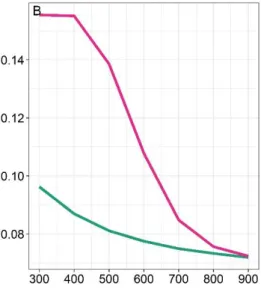
prey were vulnerable to predators, irrespectively of their body condition. To do so, we defined a 192
threshold of survival probability Th. Any adult prey with an individual survival probability pai(t) below
193
this threshold was integrated to the pool of adult prey vulnerable to predators Avuln. Rainfall and prey
194
density both affected ga(t) and thus pa(t), the mean survival probability within the population.
195
Consequently, they played a crucial role in determining the proportion of adult prey in poor body 196
condition. As pa(t) decreased, there were more adult prey with low individual survival probabilities,
197
and therefore more adult prey with a survival probability under the vulnerability threshold and exposed 198
to predation. 199
200
We integrated the influence of habitat characteristics that could affect prey vulnerability through the 201
manipulation of the handling time h, which is classically defined as the time needed by a predator to 202
subdue and consume a prey and during which the predator cannot capture another prey (Abrams & 203
Ginzburg, 2000). In our model, this time to subdue one prey corresponded to all predation attempts 204
(with one predation attempt being a predation sequence: search, encounter, and attack) leading to a 205
successful prey capture. For African savannas, we assumed that an increase in annual rainfall leads to 206
a greater vegetation cover (taller grass, more leaves in bushes and trees) and hence better concealment 207
opportunities for predators to approach their prey undetected (Hopcraft et al., 2005). Hence, we 208
considered that an increase in the climatic variable R would increase prey vulnerability, and 209
consequently decrease the number of attempts leading to a successful attack, i.e. lead to lower handling 210
time h values (an alternate situation were handling time increases with rainfall is presented in the 211
Appendix A of the Supplementary material). Therefore, h varied with rainfall according to the 212 following equation: 213 214 𝐻(𝑅) = ℎ𝑚𝑖𝑛+ℎ𝑚𝑎𝑥−ℎ𝑚𝑖𝑛 1+𝑒𝐵(𝑅−𝑉) (5) 215 216
with H(R) the value of handling time for a given year t and the rainfall value R, hmin is the lowest value
217
of h, hmax is the maximum value of h, B is the maximum rate of change, V is the rainfall value at which
218
the rate of change of h is maximum (or inflexion point). This equation allowed the handling time to 219
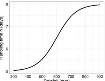
vary non-linearly and negatively with rainfall (Fig. 2C). One value of h was calculated for each rainfall 220
value and was then incorporated into the functional response I(t). 221
For the functional response, we assumed that the number of prey killed and consumed by one predator 222
during a given year t followed a type II Beddington-DeAngelis functional response. This equation 223
allows the integration of interference between predators when searching for and capturing prey and is 224
formulated as follows: 225
𝐼(𝑃(𝑡), 𝑌(𝑡)) = 𝜇𝑃(𝑡)
1+𝜏𝑌(𝑡)+𝜇ℎ𝑃(𝑡) (6)
227 228
where P(t) is the number of vulnerable prey, Y(t) the number of predators, µ a parameter defining the 229
encounter rate between predators and their prey, h the parameter defining the handling time and τ the 230
interference between predators (Abrams & Ginzburg, 2000). Finally, this type of functional response 231
allows both prey and predator densities to impact predators’ intake and therefore the regulation of 232
predator populations. 233
Predation occurs all year around. Consequently, to account for the depletion of prey that occurred 234
throughout the year and could affect the estimation of the number of prey actually captured, we 235
recursively applied the functional response presented in (6) over daily time steps, adjusting prey 236
number at each time step. We named M(t) the total number of prey killed by predators and calculated 237 it as follows: 238 239 𝑀(𝑡) = 𝑃(𝑡) − ∑365𝑑=1𝐼(𝑃(𝑑)𝑌(𝑡)) (7) 240 241
where P(t) is the number of vulnerable prey to predation, P(d) the pool of prey vulnerable to predation 242
at the beginning of day d and Y(t) the number of predators at the beginning of year t. 243
The numbers of juvenile and adult prey killed by a given predator during a year are given by: 244 245 𝑀𝑗(𝑡) = 𝑀(𝑡) × 𝐽(𝑡) 𝑃(𝑡) (8) 246 247 𝑀𝑎(𝑡) = 𝑀(𝑡) − 𝑀𝑗(𝑡) (9) 248 249
The Mj(t) juveniles killed in year t were randomly removed from the J(t) juveniles present at the
250
beginning of the year t. Similarly, the Ma(t) adults killed in year t were randomly removed from the
251
pool of vulnerable adults Avuln, i.e. individuals whose survival probabilities were below the threshold
252
of survival probability Th. For simplification, we assumed that adult and juvenile prey were equally 253
profitable to predators. Similar assumption can be found in other modelling studies (e.g. Wilmers et al. 254
2007a). 255
Finally, the predator numerical response was given by: 256
257
𝑌(𝑡 + 1) = 𝜆𝑚𝑎𝑥 × 𝑃𝑟𝑒𝑙(𝑡) × 𝑌(𝑡) (10)
258 259
where Y(t) is the number of predators present in year t, λmax is the maximum growth rate of the predator
260
population and Prel(t) was calculated as follows:
261 262 𝑃𝑟𝑒𝑙(𝑀(𝑡), 𝑌(𝑡)) = 1 𝑀(𝑡) ℎ𝑚𝑖𝑛×365×𝑌(𝑡) (11) 263
with hmin the smallest value possible for the handling time. Prel was therefore bounded between 0 and
264
1 and quantified predators hunting efficiency over a year by expressing the amount of prey actually 265
eaten in year t as a proportion of the maximum amount of prey that predators could have eaten. 266
267
3.2 Simulations
268
To study how climatic conditions may impact predator populations through their influence on prey 269
body condition or habitat characteristics, we designed 4 scenarios: 270
Scenario 1: climatic conditions influence prey availability through their effect on prey body condition 271
and ultimately on prey abundance. Prey vulnerability to predators did not vary with prey body condition 272
(all prey were vulnerable to predators) nor with habitat characteristics. Climatic conditions therefore 273
influenced predator-prey interactions only through their impacts on prey survival and fecundity, i.e. 274
through prey abundance only (blue arrows in Fig. 1). This demographic effect of climate is present in 275
all scenarios. 276
Scenario 2: prey vulnerability was affected by climatic conditions through their influence on prey body 277
condition (red arrows in Fig. 1). The poorer a prey body condition, the more vulnerable to predators 278
the prey was. Therefore, climatic conditions influence prey availability through their effect on prey 279
body condition affecting both abundance and prey vulnerability to predation. 280
Scenario 3: prey vulnerability was affected by climatic conditions through climate-driven changes in 281
habitat characteristics (e.g. vegetation) (red arrows in Fig. 1). Therefore, climatic conditions influence 282
prey availability through their effect on prey body condition affecting prey abundance and on habitat 283
characteristics affecting prey vulnerability to predation 284
Scenario 4: prey vulnerability was affected by both prey body condition and climate-driven changes 285
in habitat characteristics. In this scenario combining scenarios 2 and 3, climatic conditions influence 286
prey availability through their effect on prey body condition and habitat characteristic and, ultimately, 287
prey abundance and vulnerability to predation. 288
While in scenarios 1 and 3 predators could capture any prey individual, in scenarios 2 and 4 289
predators could capture any juvenile, but could only subdue adult prey that were in poor body 290
condition. These differences between scenarios were modelled by setting the value of the threshold of 291
survival probability Th at 1 in scenario 1 and 3, and at 0.5 in scenario 2 and 4 (Table 1). As vulnerability 292
to predators was independent from habitat characteristics in scenarios 1 and 2, the handling time was 293
set constant and equal to h = 5 in these scenarios. In scenarios 3 and 4, prey vulnerability to predators 294
was dependent on habitat characteristics and handling time h varied with climatic conditions following 295
equation 5 (for a summary of the model functioning see Fig. 3). 296
We focused on these 4 scenarios only, as the goal of this study was to assess how the addition 297
of prey vulnerability to traditional predator-prey models that considered prey abundance only would 298
change the expectations in terms of responses of predator populations to climatic changes. 299
300
For simulations, parameters were given default values considered realistic for African large mammals. 301
These default values and initial values for state variables are presented Table 1. The sensitivity of the 302
main results to some of these parameter values was investigated by sensitivity analyses (see section 303
below). As we were mostly interested in how the link between climatic conditions and prey 304
vulnerability could affect predator dynamics, predators were characterized by identical parameter 305
values in the different scenarios, but for the threshold Th and handling time h values. Therefore, in our 306
work, all differences in predator dynamics between scenarios emerged from differences in these two 307
parameters. 308
3.2.1 Immediate response of predator populations to specific rainfall conditions
309
We assessed, for each scenario, the immediate response of the predator population to specific rainfall 310
conditions. We simulated over 198 years the dynamics of the predator population under the long-term 311
annual rainfall 600 mm, then imposed a predefined rainfall in year 199 (different values were tested: 312
from 300mm to 900mm, by 100mm increments), and calculated the predator population growth rate 313
over that year (calculated as λ = Yt+1/Yt). To obtain robust estimates of predator population growth
314
rates and account for within-simulation variability in prey demographic rates, each simulation, 315
characterized by a long-term annual rainfall value of 600mm and one predefined rainfall for the last 316
year, was replicated 1000 times. 317
3.2.2 Long-term response of predator populations to changes in mean annual rainfall
318
We assessed, for each scenario, how a change in mean annual rainfall may affect predator populations 319
on the long run. We compared the average predator population size (over the last twenty-one years of 320
a 200-year simulation) across simulations run under different long-term rainfall averages. The mean 321
annual rainfall values varied from 300mm to 900mm, by 100mm increments. For each value, 322
simulations were replicated 1000 times, allowing again to account for within simulation variability in 323
prey demographic rates. 324
3.2.3 Sensitivity analyses
325
Because model outcomes can be sensitive to the choice of parameter values, we conducted sensitivity 326
analyses for some model parameters. We first investigated the effect of changes in parameter hmin and
327
Th, which are of importance because differences between scenarios originate from these two 328
parameters. In addition, we also tested for the influence of changes in λmax values, which is a central
329
parameter of the predator numerical response. Finally, we carried out a sensitivity analysis for the δ 330
parameter, which describes the shape of density dependence and determines the magnitude of the prey 331
population response, the number of individuals per resource units, and ultimately prey dynamics. We 332
always varied this parameter simultaneously for adult and juvenile, ensuring that juvenile survival 333
never exceeded adult survival (see Fig. 2A). Sensitivity analyses were conducted by increasing or 334
decreasing each of these parameters, one at a time, by 20 percent around its default value. For each 335
parameter value, simulations were replicated 500 times. Results of the sensitivity analyses are 336
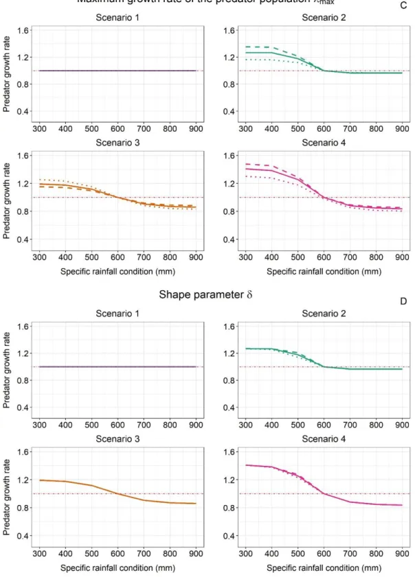
presented in the Appendix B of the Supplementary Material. 337
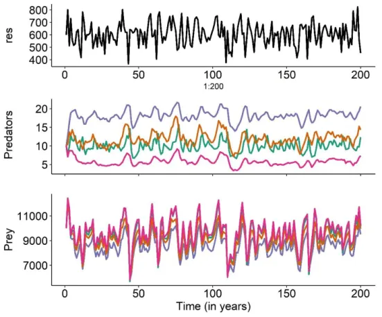
An example of the behaviour of the model for one run showing fluctuations of rainfall, prey and 338
predator population size over 200 years is presented in Fig. S7 (Appendix C of the Supplementary 339
Material) and a summary of the key steps of the modelling process and of the different scenarios can 340
be found in Fig. 3. All simulations were conducted in R 4.0.2 (R Core Team, 2020). 341
4 Results
342
4.1 Immediate response of predator populations to specific rainfall conditions
343
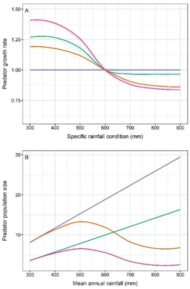
In scenario 1, i.e. when climatic conditions influenced prey abundance only (through survival and 344
fecundity) and not prey vulnerability, the population growth rate of predators was not influenced by 345
the specific climatic condition of the year (Fig. 4A). This result was not surprising as according to the 346
model design, the demographic consequences of climate are expected to be visible in prey population 347
the following year (t+1) and, therefore, would only impact predator growth rate calculated over the 348
year t+1 and t+2. In contrast, in the three other scenarios, i.e. when climatic conditions influenced prey 349
vulnerability, either through changes in prey body condition (scenario 2) or through changes in habitat 350
characteristics (scenario 3) or both (scenario 4), the population growth rate of predators one year was 351
influenced by the specific climatic condition of the year. Population growth rates in scenarios 2 and 3 352
showed opposite patterns (Fig. 4A). Predators from scenario 2 benefited from below-average rainfall 353
(600mm) and their populations increased, as shown by the growth rate being greater than 1, but there 354
was a negative effect of above-average rainfall (Fig. 4A). In scenario 3, there was a negative effect of 355
below-average rainfall and a positive effect of above-average rainfall on predator growth rate (Fig. 356
4A). Because scenario 4 is a combination of scenarios 2 and 3, the population growth rate of predators 357
from scenario 4 was intermediate between those of scenarios 2 and 3 (Fig. 4A). 358
4.2 Long-term response of predator populations to changes in mean annual rainfall
Our results showed an effect of mean annual rainfall on the size of predator populations for all 360
scenarios, but the shape of the relationships varied. In scenario 1 (when climatic conditions influenced 361
prey abundance only), the size of predator populations increased near-linearly with rainfall (Fig. 4B). 362
As expected because all individuals were vulnerable to predation, the size of predator populations in 363
this scenario was always greater than the one observed in other scenarios. The size of predator 364
populations in scenario 2 (when climatic conditions influenced prey vulnerability through changes in 365
prey body condition only) also increased near-linearly with mean annual rainfall. It was consistently 366
lower than the size of the predator population in scenario 1 because only a fraction of the prey 367
population is vulnerable to predation in scenario 2. However, the effect of climatic conditions on 368
predator population sizes was weaker in scenario 2 than in scenario 1: as the amount of rainfall 369
increased, the difference between scenarios 1 and 2 in the size of predator populations increased (Fig. 370
4B). Conversely, the size of predator populations varied non-linearly with increasing rainfall in 371
scenario 3, when climatic conditions influenced prey vulnerability through changes in habitat 372
characteristics only, and in scenario 4, when climatic conditions influenced prey vulnerability through 373
both changes in prey body condition and habitat characteristics. More specifically, the size of predator 374
populations in scenario 3 were smaller than those from scenario 2 up until mean annual rainfall reached 375
values around 600mm, but were greater for values above (Fig. 4B). In addition, for mean annual rainfall 376
of 900mm, the size of predator populations in scenario 1 and 3 were almost equal. In scenario 4, 377
changes in the size of predator populations with increasing mean annual rainfall generally followed a 378
similar pattern than those observed from the scenario 3. However, the difference in the size of predator 379
populations between scenario 4 and 3 increased with increasing rainfall (Fig. 4B). Conversely, the size 380
of predator populations were virtually identical between scenario 4 and 2 at the wettest end of the 381
rainfall gradient (Fig. 4B). In all cases, the size of predator populations in scenario 4 was always equal 382
or lower than in the other scenarios (Fig. 4B). 383
5 Discussion
384
Our work shows how predator populations could respond differently to changing climatic conditions 385
depending on how climate influences prey vulnerability (habitat characteristics vs. body condition). 386
For example, in a context of aridification, a predator-prey system where prey vulnerability depends 387
mainly on prey body condition (scenario 2) would be characterized by larger predator populations than 388
a system where prey vulnerability is mainly affected by the habitat (scenario 3) (see section 5.1 for the 389
role of species traits). It thus highlights the importance of having a good understanding of the processes 390
determining vulnerability at play within the predator-prey pair studied, as integrating climate influence 391
on prey vulnerability, in addition to resource-mediated climate effects on prey abundance, leads to 392
different responses of predator populations (on the short- and the long-term) to changes in climatic 393
conditions. 394
5.1 How species traits influence the relative importance of the different sources of
395
vulnerability
396
Ultimately, whether the predator-prey pair studied will respond according to one scenario or another 397
will depend upon the traits of the species involved. Here, we will illustrate the importance of the 398
predator hunting mode and the prey escape tactics, as well as the importance of the relative size of the 399
predator and the prey. Predator hunting mode (cursorial or ambush) and prey escape tactics (fleeing, 400
fighting or freezing) are key behavioural traits involved in predator-prey interactions that can affect 401
how climatic conditions contribute, indirectly via forage resources or vegetation cover, to determine 402
the vulnerability of prey to predation. For example, cursorial predators, such as spotted hyaenas 403
Crocuta crocuta (Cooper, 1990) and wild dogs Lycaon pictus (Pole et al., 2004) in African savannas, 404
or wolves in temperate ecosystems (Mech et al., 2015), are active predators, i.e. they can chase down 405
their prey over long distances and are more likely to kill individuals in poor body condition. They 406
therefore exemplify predators from scenario 2 (climatic conditions influence prey vulnerability through 407
changes in prey body condition only), as prey in poorer condition because of a shortage of food will 408
be particularly more vulnerable to predation from these predators (Atwood et al., 2007; Mills, 1995; 409
Pole et al., 2004). Conversely, ambush predators, such as African lions Panthera leo and leopards 410
Panthera pardus in African savannas, or cougars Puma concolor and lynx Lynx lynx in temperate 411
ecosystems, stalk their prey before attacking them by surprise when they come within short distance 412
(Elliott et al., 1977; Husseman et al., 2003). As such, they rely less on prey body condition. However, 413
to approach their prey undetected, ambush predators need concealment. Therefore, their hunting 414
success is prone to be influenced by vegetation (Funston et al., 2001; Lone et al., 2014), and negatively 415
affected by an increased aridity and a subsequent decrease in vegetation density (scenario 3, climatic 416
conditions influence prey vulnerability through changes in habitat characteristics only). Whereas prey 417
escape tactics might not be that crucial for the outcome of an encounter with an ambush predator, a 418
climate-driven decrease in prey body condition will negatively influence prey fleeing capacity leading 419
to an overall disadvantage against cursorial predators (scenario 2). 420
Predator body size influences the prey body size targeted by the predator (Owen-Smith & Mills, 421
2008a; Radloff & du Toit, 2004) and climate-driven changes in prey body condition can interfere with 422
the chance of successfully subduing an adult prey depending on the relative size of the predator and 423
the prey considered (Mech et al., 2001; Metz et al., 2012). For example, for lion-impala interactions, it 424
is very likely that climatic conditions will not affect the likelihood of lions to capture an adult impala 425
Aepyceros melampus, while in the case of lion-buffalo Syncerus caffer interactions, lions are expected 426
to successfully hunt adult buffaloes, which are dangerous prey for them, in dry conditions only 427
(scenario 2, Owen-Smith, 2008). This is also true at the interspecific level: prey species that are usually 428
inaccessible because they are too difficult to be captured under normal climatic conditions may become 429
vulnerable due to unfavourable conditions, allowing predators to kill young individuals of larger 430
species (e.g. with elephants: Loveridge et al., 2006; Salnicki et al., 2001). 431
432
5.2 Importance of integrating climate-driven changes in prey vulnerability
433
Our results show how predator population responses to changes in climatic conditions differ when we 434
take into account climate-driven changes in prey vulnerability in addition to climate-driven changes in 435
prey abundance (existing work take into account climate-driven changes in prey abundance only – Fig. 436
1). For example, while the overall trend depicted in all 4 scenarios on the long-term is that there are 437
more predators when rainfall increases, because of an overall increase in prey population abundance, 438
the originality of our study is to illustrate how prey vulnerability and its drivers influence the link 439
between predator populations and climate. 440
When changes in climatic conditions influence prey vulnerability through changes in prey body 441
condition (scenario 2), a below average rainfall event leads to poorer herbivore body condition, and 442
hence results in an increase in the pool of adult prey vulnerable to predators (Fig. S8A). Unsurprisingly, 443
this, in turn, favours the immediate growth rate of the predator population. This result is in accordance 444
with field observations, which reported a positive effect of drought conditions over the short-term on 445
large carnivore populations (Mills, 1995). These dry-condition increases in prey vulnerability can be 446
assimilated to “resource pulses” for the predators and to be beneficial to them (Holt, 2008; Yang et al., 447
2008). Contrarily, above average rainfall events negatively affects the population growth rate of 448
predators, as very few prey adults are vulnerable in years characterized by high levels of resources 449
(Fig. S8A). Over the long term, predator populations benefit from the overall increase in prey 450
populations associated with increasing rainfall (Fig. S9). However, predators in scenario 2 can only 451
subdue a portion of adult prey and have a smaller pool of available prey than predators in scenario 1. 452
They are therefore maintained at smaller population size. In addition, the proportion of vulnerable adult 453
prey decreases with increasing rainfall (Fig. S8B), which leads to the observed increase in the 454
difference between the size of predator populations in scenario 1 and 2. 455
When changes in climatic conditions influence prey vulnerability through changes in habitat 456
characteristics and habitat-driven hunting success increases with rainfall (scenario 3), predator growth 457
rates are negatively impacted by below average rainfall and positively influenced by above average 458
rainfall. This is typically the case in African savannas where grass height is related to rainfall 459
(Rutherford, 1980) and lions are hunters that are more successful in tall grass (Funston et al., 2001). 460
Over the long term, predator populations benefit from the combined linear increase of prey abundance 461
(Fig. S9) and non-linear increase of hunting success (i.e. decrease of handling time, Fig. 2C), leading 462
to an overall non-linear increase as rainfall increases. 463
Finally, when changes in climatic conditions influence prey vulnerability through changes in 464
both prey body condition and habitat characteristics (scenario 4), the growth rate of predator 465
populations combines the effects of both sources of vulnerability and predators are affected by opposite 466
effects of different sources of vulnerability. For below average rainfall, predators benefit from the 467
positive effect of lower prey body conditions, which buffers the negative effect of a lower hunting 468
success due to habitat characteristics, and inversely for above rainfall level, leading to the observed 469
intermediate pattern of predator growth rate (Fig. 4A, Fig. 2C, Fig. S8A). Over the long term, predator 470
populations of scenario 4 follow the same patterns as the populations in scenario 3 with the exception 471
that they can only subdue a proportion of adult prey. They subsequently remain at a smaller population 472
size. 473
5.3 Contrasting predator responses to short- and long-term climate fluctuations
474
Our study highlights the importance of the temporal scale considered as the patterns observed differed 475
whether we considered the short- or long-term temporal scale. While a sudden arid event can be 476
beneficial to predator population, increasing aridity over time leads to an overall decrease in predator 477
population size. The explanation of such differences lies in the fact that a predator response over the 478
long term integrates the predator responses over the short-term, along with the long-term response of 479
prey, which declines with increasing aridity (Fig. S9). Therefore, our results illustrate that the long-480
term response of predator populations to changes in mean annual rainfall cannot be predicted only from 481
the immediate response of predator populations to specific rainfall conditions. 482
483
5.4 Considerations on the model
484
Modelling studies are difficult exercises where one walk on a thin line between complexity/realism 485
and simplification that is required for conceptualization, i.e. building some theoretical understanding. 486
We have tried to do this successfully but we want to underline here a few simplifications made in this 487
study (and already made in classical models of predator-prey interactions – e.g. Wilmers et al., 2007a, 488
b). It is noteworthy that the code of the model is available (https://github.com/aissamorin/climate-prey-489
vulnerability-and-predators) so that one can parametrize it for a specific system and add the complexity 490
that would be considered critical. First, in our model, juvenile prey contribute as much energy as adult 491
prey. Second, the predator population is not age-structured. Third, the predator-prey system modelled 492
here involves one prey and one predator only, yet multi-species assemblages often characterize both 493
prey and predator communities. Predators often prey on several prey species, with primary and 494
secondary prey and display prey switching depending on prey availability and catchability (Owen-495
Smith & Mills 2008b, Elbroch et al. 2013). The presence of an alternative prey could influence model 496
outcomes for scenarios 2, 3 and 4: when the vulnerability of the primary prey decreases, if the predator 497
can switch to an alternate prey species available and more vulnerable, the decrease in predator 498
population growth rate or over the long term may be weaker or not observed. In contrast, the presence 499
of competitors preying on the same prey could intensify the decrease in the number of vulnerable prey 500
available to each predator owing to additive effects (Melis et al. 2009), and negatively influence 501
predator population size. 502
5.5 Conclusion
503
Despite its general simplicity, this theoretical study highlights the importance of understanding, and 504
accounting for, the vulnerability factors in predator-prey relationships, and sheds light on the 505
complexity of predicting predator-prey relationships in a changing climate. We believe it is a 506
prospective study that suggests interesting future research directions. Based on our work, we advise 507
that future theoretical and empirical works should integrate climate-driven changes in prey 508
vulnerability if we want to grasp the full picture of the impacts of climate changes on predator-prey 509
interactions. 510
6 Conflict of Interest
511
The authors declare that the research was conducted in the absence of any commercial or financial 512
relationships that could be construed as a potential conflict of interest. 513
7 Funding
514
This work was partly funded by the Agence Nationale de la Recherche (project Landthirst ANR-16-515
CE02-0001-01 and FUTURE-PRED ANR-18-CE02-0005-01) and was further supported by a grant 516
from the “Ministère français de lʼEnseignement supérieur, de la Recherche et de lʼInnovation” through 517
the “Ecole Doctorale E2M2” of “Université Claude Bernard Lyon 1”. 518
8 Author contributions
519
MV and SC conceived the ideas; AM and SC designed the model. All authors analysed the results, 520
wrote the manuscript, and gave approval for publication. 521
9 Acknowledgments
522
We thank C. Wilmers for providing the code of the published model that serves as the basis of ours. In 523
addition, this work benefited from the computing cluster platform of the Centre d’Ecologie 524
Fonctionnelle et Evolutive and from Biosphere, the IFB cloud for life sciences. We thank Bruno 525
Spataro and Stéphane Delmotte from the LBBE computing services for their help in using computing 526
facilities. Finally, we thank two anonymous reviewers for their fruitful comments on a previous draft 527
of this manuscript. 528
529
10 Data availability statement
530
The code used for the model and the simulations is available from a GitHub repository: 531
https://github.com/aissamorin/climate-prey-vulnerability-and-predators. 532
11 Literature cited
Abrams, P. A., and Ginzburg, L. R. (2000). The nature of predation: prey dependent, ratio dependent or 534
neither? Trends Ecol. Evol. 15, 337–341. doi:10.1016/S0169-5347(00)01908-X. 535
Atwood, T. C., Gese, E. M., and Kunkel, K. E. (2007). Comparative patterns of predation by cougars and 536
recolonizing wolves in Montana’s Madison Range. J. Wildl. Manage. 71, 1098–1106. 537
doi:10.2193/2006-102. 538
Bastille-Rousseau, G., Schaefer, J. A., Peers, M. J. L., Ellington, E. H., Mumma, M. A., Rayl, N. D., et 539
al. (2018). Climate change can alter predator-prey dynamics and population viability of prey. 540
Oecologia 186, 141–150. doi:10.1007/s00442-017-4017-y. 541
Bayliss, P., and Choquenot, D. (2002). The numerical response: rate of increase and food limitation in 542
herbivores and predators. Philos. Trans. R. Soc. B Biol. Sci. 357, 1233–1248. 543
doi:10.1098/rstb.2002.1124. 544
Bender, L. C., Lomas, L. A., and Browning, J. (2007). Condition, survival, and cause-specific mortality 545
of adult female Mule deer in North-Central New Mexico. J. Wildl. Manage. 71, 1118–1124. 546
doi:10.2193/2006-226. 547
Bonenfant, C., Gaillard, J. M., Coulson, T., Festa-Bianchet, M., Loison, A., Garel, M., et al. (2009). 548
“Empirical Evidence of Density-Dependence in Populations of Large Herbivores,” in Advances 549
in Ecological Research, 313–357. doi:10.1016/S0065-2504(09)00405-X. 550
Bourgarel, M., Fritz, H., Gaillard, J. M., De Garine-Wichatitsky, M., and Maudet, F. (2002). Effects of 551
annual rainfall and habitat types on the body mass of impala (Aepyceros melampus) in the Zambezi 552
Valley, Zimbabwe. Afr. J. Ecol. 40, 186–193. doi:10.1046/j.1365-2028.2002.00377.x. 553
Candolin, U., and Wong, B. B. M. (2012). Behavioural Responses to a Changing World. First. Oxford: 554
Oxford University Press. 555
Carbone, C., and Gittleman, J. L. (2002). A Common Rule for the Scaling of Carnivore Density. Science 556
. 295, 2273–2276. doi:10.1126/science.1067994. 557
Caswell, H. (2001). Matrix population models: construction, analysis, and interpretation. Second edi. 558
Sunderland, Massachusetts: Sinauer Associates. 559
Chamaillé-Jammes, S., and Fritz, H. (2009). Precipitation-NDVI relationships in eastern and southern 560
African savannas vary along a precipitation gradient. Int. J. Remote Sens. 30, 3409-3422. doi: 561
10.1080/01431160802562206. 562
Cook, J. G., Johnson, B. K., Cook, R. C., Riggs, R. A., Delcurto, T., Bryant, L. D., et al. (2004). Effects 563
of Summer-Autumn Nutrition and Parturition Date on Reproduction and Survival of Elk. Wildl. 564
Monogr. 155, 1–61. doi:10.2193/0084-0173(2004)155[1:EOSNAP]2.0.CO;2. 565
Cooper, S. M. (1990). The hunting behaviour of spotted hyaenas (Crocuta crocuta) in a region containing 566
both sedentary and migratory populations of herbivores. Afr. J. Ecol. 28, 131–141. 567
doi:10.1111/j.1365-2028.1990.tb01145.x. 568
East, R. (1984). Rainfall, soil nutrient status and biomass of large African savanna mammals. Afr. J. Ecol. 569
22, 245–270. doi:10.1111/j.1365-2028.1984.tb00700.x. 570
Eberhardt, L. L. (1977). Optimal policies for conservation of large mammals, with special reference to 571
marine ecosystems. Environ. Conserv. 4, 205–212. doi:10.1017/S0376892900025819. 572
Elbroch, L. M., Lendrum, P. E., Newby, J., Quigley, H., and Craighead, D. (2013). Seasonal foraging 573
ecology of non-migratory cougars in a system with migrating prey. PLoS One 8, 1–14. 574
doi:10.1371/journal.pone.0083375. 575
Elliott, J. P., Cowan, I. M., and Holling, C. S. (1977). Prey capture by the African lion. Can. J. Zool. 55, 576
1811–1828. doi:10.1139/z77-235. 577
Estes, R. (1991). The behavior guide to African mammals: including hoofed mammals, carnivores, 578
primates. University of California Press. 579
Fitzgibbon, C. D., and Fanshawe, J. H. (1989). The condition and age of Thomson’s gazelles killed by 580
cheetas and wild dogs. J. Zool. 218, 99–107. doi:10.1111/j.1469-7998.1989.tb02528.x. 581
Foley, C., Pettorelli, N., and Foley, L. (2008). Severe drought and calf survival in elephants. Biol. Lett. 582
4, 541–544. doi:10.1098/rsbl.2008.0370. 583
Forchhammer, M. C., Stenseth, N. C., Post, E., and Langvatn, R. (1998). Population dynamics of 584
Norwegian red deer: density-dependence and climatic variation. Proc. R. Soc. B Biol. Sci. 265, 585
341–350. doi:10.1098/rspb.1998.0301. 586
Funston, P. J., Mills, M. G. L., and Biggs, H. C. (2001). Factors affecting the hunting success of male and 587
female lions in the Kruger National Park. J. Zool. 253, 419–431.
588
doi:10.1017/S0952836901000395. 589
Grange, S., Barnier, F., Duncan, P., Gaillard, J. M., Valeix, M., Ncube, H., et al. (2015). Demography of 590
plains zebras (Equus quagga) under heavy predation. Popul. Ecol. 57, 201–214. 591
doi:10.1007/s10144-014-0469-7. 592
Holling, C. S. (1959). The Components of Predation as Revealed by a Study of Small-Mammal Predation 593
of the European Pine Sawfly. Can. Entomol. 91, 293–320. doi:10.4039/Ent91293-5. 594
Holt, R. D. (2008). Theoretical perspectives on resource pulses. Ecology 89, 671–681. doi:10.1890/07-595
0348.1. 596
Hopcraft, Grant, J. C., Sinclair, A. R. E., and Packer, C. (2005). Planning for success: Serengeti lions seek 597
prey accessibility rather than abundance. J. Anim. Ecol. 74, 559–566. doi:10.1111/j.1365-598
2656.2005.00955.x. 599
Husseman, J. S., Murray, D. L., Power, G., Mack, C., Wenger, C. R., and Quigley, H. (2003). Assessing 600
differential prey selection patterns between two sympatric large carnivores. Oikos 101, 591–601. 601
doi:10.1034/j.1600-0706.2003.12230.x. 602
Inouye, D. W., Barr, B., Armitage, K. B., and Inouye, B. D. (2000). Climate change is affecting altitudinal 603
migrants and hibernating species. Proc. Natl. Acad. Sci. 97, 1630–1633.
604
doi:10.1073/pnas.97.4.1630. 605
IPCC. (2014a). Summary for Policymakers. Geneva, Switzerland: IPCC
606
doi:10.1017/CBO9781107415324. 607
IPCC. (2014b). “Climate Change 2014: Impacts, Adaptation, and Vulnerability. Part B: Regional Aspects. 608
Contribution of Working Group II to the Fifth Assessment Report of the Intergovernmental Panel 609
on Climate Change,” in (Cambridge: Cambridge University Press), 688. 610
Lone, K., Loe, L. E., Gobakken, T., Linnell, J. D. C., Odden, J., Remmen, J., et al. (2014). Living and 611
dying in a multi-predator landscape of fear: roe deer are squeezed by contrasting pattern of 612
predation risk imposed by lynx and humans. Oikos 123, 641–651. doi:10.1111/j.1600-613
0706.2013.00938.x. 614
Loveridge, A. J., Hunt, J. E., Murindagomo, F., and Macdonald, D. W. (2006). Influence of drought on 615
predation of elephant (Loxodonta africana) calves by lions (Panthera leo) in an African wooded 616
savannah. J. Zool. 270, 523–530. doi:10.1111/j.1469-7998.2006.00181.x. 617
Maclean, I. M. D., and Wilson, R. J. (2011). Recent ecological responses to climate change support 618
predictions of high extinction risk. Proc. Natl. Acad. Sci. 108, 12337–12342. 619
doi:10.1073/pnas.1017352108. 620
Martay, B., Brewer, M. J., Elston, D. A., Bell, J. R., Harrington, R., Brereton, T. M., et al. (2017). Impacts 621
of climate change on national biodiversity population trends. Ecography (Cop.). 40, 1139–1151. 622
doi:10.1111/ecog.02411. 623
Mduma, S. A. R., Sinclair, A. R. E., and Hilborn, R. (1999). Food regulates the Serengeti wildebeest: A 624
40-year record. J. Anim. Ecol. 68, 1101–1122. doi:10.1046/j.1365-2656.1999.00352.x. 625
Mech, D. L., Smith, D. W., Murphy, K. M., and MacNulty, D. R. (2001). Winter severity and wolf 626
predation on a formerly wolf- free elk herd. J. Wildl. Manage. 65, 998–1003. 627
doi:10.2307/3803048. 628
Mech, L. D., Frenzel, D. J., and Karns, P., D. (1971). “The effect of snow conditions on the vulnerability 629
of white-tailed deer to wolf predation,” in Ecological studies of the timber wolf in northeastern 630
Minnesota, eds. L. D. Mech and D. J. Frenzel (North Central Forest Experimental Station, St. 631
Paul, Minnesota: USDA Forest Service Research Paper NC-52), 51–59. 632
Mech, L. D., Smith, D. W. and MacNulty, D. R. (2015). “Introduction The Wolf as a Killing Machine,” 633
in Wolves on the hunt the behavior of wolves hunting wild prey, eds. D. R. Mech, L. D., Smith, 634
D. W. and MacNulty (Chicago: The University of Chicago Press), 1–9. 635
Melis, C., Jȩdrzejewska, B., Apollonio, M., Bartoń, K. A., Jȩdrzejewski, W., Linnell, J. D. C., et al. 636
(2009). Predation has a greater impact in less productive environments: Variation in roe deer, 637
Capreolus capreolus, population density across Europe. Glob. Ecol. Biogeogr. 18, 724–734. 638
doi:10.1111/j.1466-8238.2009.00480.x. 639
Metz, M. C., Smith, D. W., Vucetich, J. A., Stahler, D. R., and Peterson, R. O. (2012). Seasonal patterns 640
of predation for gray wolves in the multi-prey system of Yellowstone National Park. J. Anim. 641
Ecol. 81, 553–563. doi:10.1111/j.1365-2656.2011.01945.x. 642
Mills, M. G. L. (1995). Notes on wild dog Lycaon pictus and lion Panthera leo population trends during 643
a drought in the Kruger National Park. Koedoe 38, 95–99. doi:10.4102/koedoe.v38i1.309. 644
Moyes, K., Nussey, D. H., Clements, M. N., Guinness, F. E., Morris, A., Morris, S., et al. (2011). 645
Advancing breeding phenology in response to environmental change in a wild red deer population. 646
Glob. Chang. Biol. 17, 2455–2469. doi:10.1111/j.1365-2486.2010.02382.x. 647
Mysterud, A., Stenseth, N. C., Yoccoz, N. G., Langvatn, R., and Steinheim, G. (2001). Nonlinear effects 648
of large-scale climatic variability on wild and domestic herbivores. Nature 410, 1096–1099. 649
doi:10.1038/35074099. 650
Ogutu, J. O., Piepho, H.-P., Dublin, H. T., Bhola, N., and Reid, R. S. (2008). Rainfall influences on 651
ungulate population abundance in the Mara-Serengeti ecosystem. J. Anim. Ecol. 77, 814–829. 652
doi:10.1111/j.1365-2656.2008.01392.x. 653
Owen-smith, N. (1990). Demography of a large herbivore, the greater kudu tragelaphus strepsiceros, in 654
relation to rainfall. J. Anim. Ecol. 59,893-829. doi:10.2307/5021. 655
Owen-smith, N. (2008). Changing vulnerability to predation related to season and sex in an African 656
ungulate assemblage. Oikos 117, 602–610. doi: 10.1111/j.0030-1299.2008.16309.x. 657
Owen-Smith, N. (2002). Adaptive herbivore ecology from resources to populations in variable 658
environments. Cambridge: Cambridge University Press doi:10.1017/CBO9780511525605. 659
Owen-Smith, N., and Mills, M. G. L. (2008a). Predator-prey size relationships in an African large-660
mammal food web. J. Anim. Ecol. 77, 173–183. doi:10.1111/j.1365-2656.2007.01314.x. 661
Owen-Smith, N., and Mills, M. G. L. (2008b). Shifting prey selection generates contrasting herbivore 662
dynamics within a large-mammal predator-prey web. Ecology 89, 1120–1133. doi:10.1890/07-663
0970.1. 664
Pacifici, M., Visconti, P., Butchart, S. H. M., Watson, J. E. M., Cassola, F. M., and Rondinini, C. (2017). 665
Species’ traits influenced their response to recent climate change. Nat. Clim. Chang. 7, 205–208. 666
doi:10.1038/nclimate3223. 667
Parmesan, C., Ryrholm, N., Stefanescu, C., Hill, J. K., Thomas, C. D., Descimon, H., et al. (1999). 668
Poleward shifts in geographical ranges of butterfly species associated with regional warming. 669
Nature 399, 579–583. doi:10.1038/21181. 670
Pole, A., Gordon, I. J., Gorman, M. L., and MacAskill, M. (2004). Prey selection by African wild dogs 671
(Lycaon pictus) in southern Zimbabwe. J. Zool. 262, 207–215. doi:10.1017/S0952836903004576. 672
Post, E., Peterson, R. O., Stenseth, N. C., and McLaren, B. E. (1999). Ecosystem consequences of wolf 673
behavioural response to climate. Nature 401, 905–907. doi:10.1038/44814. 674
Post, E., and Stenseth, N. C. (1999). Climatic Variability, Plant Phenology , and Northern ungulates. 675
Ecology 80, 1322–1339. doi: 10.1890/0012-9658(1999)080[1322:CVPPAN]2.0.CO;2. 676
Radloff, F. G. T., and Du Toit, J. T. (2004). Large predators and their prey in a southern African savanna: 677
a predator’s size determines its prey size range. J. Anim. Ecol. 73, 410–423. doi:10.1111/j.0021-678
8790.2004.00817.x. 679
R Core Team (2020). R: A language and environment for statistical computing. R Foundation for 680
Statistical Computing, Vienna, Austria. 681
Rutherford, M. C. (1980). Annual plant production precipitation relations in Arid and Semi-arid regions. 682
S. Afr. J. Sci. 76, 53–57. 683
Saether, B.-E. (1997). Environmental stochasitcity and population dynamics of large herbivores: a search 684
for mechanisms. Trends Ecol. Evol. 12, 143–149. doi:10.1016/S0169-5347(96)10068-9. 685
Saether, B.-E., and Gravem, A. J. (1988). Annual variation in winter body condition of Norwegian moose 686
calves. J. Wildl. Manage. 52, 333–336. doi:10.2307/3801245. 687
Salnicki, J., Teichmann, M., Wilson, V., and J. and Murindagomo, F. (2001). Spotted hyaenas Crocuta 688
crocuta prey on new-born elephant calves in Hwange National Park, Zimbabwe. Koedoe 44, 79– 689
83.doi: 10.4102/koedoe.v44i2.177. 690
Sankaran, M., Hanan, N. P., Scholes, R. J., Ratnam, J., Augustine, D. J., Cade, B. S., et al. (2005). 691
Determinants of woody cover in African savannas. Nature 438, 846–849.
692
doi:10.1038/nature04070. 693
Schaller, G. B. (1972). The Serengeti Lion A study of Predator-Prey Relations. First. Chicago: The 694
University of Chicago Press. 695
Stenseth, N. C., Shabbar, A., Chan, K., Boutin, S., Rueness, E. K., Ehrich, D., et al. (2004). Snow 696
conditions may create an invisible barrier for lynx. Proc. Natl. Acad. Sci. 101, 10632–10634. 697
doi:10.1073/pnas.0308674101. 698
Visser, M. E., Holleman, L. J. M., and Gienapp, P. (2006). Shifts in caterpillar biomass phenology due to 699
climate change and its impact on the breeding biology of an insectivorous bird. Oecologia 147, 700
164–172. doi:10.1007/s00442-005-0299-6. 701
Wilmers, C. C., Post, E., and Hastings, A. (2007a). The anatomy of predator-prey dynamics in a changing 702
climate. J. Anim. Ecol. 76, 1037–1044. doi:10.1111/j.1365-2656.2007.01289.x. 703
Wilmers, C. C., Post, E., and Hastings, A. (2007b). A perfect storm: The combined effects on population 704
fluctuations of autocorrelated environmental noise, age structure, and density dependence. Am. 705
Nat. 169, 673–683. doi:10.1086/513484. 706
Yang, L. H., Bastow, J. L., Spence, K. O., and Wright, A. N. (2008). What can we learn from resource 707
pulses? Ecology 89, 621–634. doi:10.1890/07-0175.1. 708
12 Table
710
Table 1: Definitions and values of the state variables and parameters for prey and predators used in the model.
711
Variables Definition/description Values
𝑁(𝑡) Prey population size at the beginning of year t N1=10000
𝐽(𝑡) Number of juvenile prey at the beginning of year t J1=2500
𝐴(𝑡) Number of adult prey at the beginning of year t A1=7500
𝑌(𝑡) Predator population size at the beginning of year t Y1=10
𝑃(𝑡) Pool of prey vulnerable to predation for year t Calculated at each time step
𝑀(𝑡) Pool of prey consumed at the end of year t Calculated at each time step
𝛼𝑎 First shape parameter of the Beta distribution from which are drawn adult prey
individual survival rate Calculated at each time step
𝛼𝑗 First shape parameter for Beta distribution from which are drawn juvenile prey
individual survival rate Calculated at each time step
𝛽𝑎 Second shape parameter for Beta distribution from which are drawn adult prey
individual survival rate Calculated at each time step
𝛽𝑗
Second shape parameter for Beta distribution from which are drawn juvenile
prey individual survival rate Calculated at each time step
𝑃𝑎 Maximum adult prey survival probability 0.95
𝑃𝑗 Maximum juvenile prey survival probability 0.8
𝑆𝑑𝑝𝑎 Standard deviation, variation of adult prey survival 0.05
𝑆𝑑𝑝𝑗 Standard deviation, variation of juvenile prey survival 0.05
𝑔𝑎 Effect of increased population density on adult survival 𝑔(𝑁(𝑡)) =
𝛾𝑃𝑎𝛿𝑃𝑎
𝛾𝑃𝑎𝛿𝑃𝑎+𝑁(𝑡)
𝑅
𝑔𝑗 Effect of increased population density on juvenile survival 𝑔(𝑁(𝑡)) =
𝛾𝑃𝑗𝛿𝑃𝑗 𝛾𝑃𝑗𝛿𝑃𝑗+𝑁(𝑡)𝑅
𝑝𝑗 Mean juvenile prey survival probability 𝑝𝑗 = 𝑃𝑗 × 𝑔𝑗
𝛾𝑃𝑎 Adult half-saturation, point at which adult prey survival is lowered by half 30
𝛾𝑃𝑗 Juvenile half-saturation, point at which juvenile prey survival is lowered by half 20
𝛿𝑃𝑎 Shape parameter, defines the onset of density-dependence for adult prey 2
𝛿𝑃𝑗 Shape parameter, defines the onset of density-dependence for juvenile prey 2
𝑅 Annual level of rainfall Varies between 300 & 900mm,
by 100mm increment
𝐹𝑙𝑜𝑤 Value determining fecundity value when adult survival is close to 0 100
𝐹𝑔𝑟𝑜𝑤𝑡ℎ Rate at which fecundity value reaches 1 15
𝑇ℎ Prey threshold of survival probability below which predators can catch and consume the prey.
𝑇ℎ = 1 for scenarios 1 & 3; 𝑇ℎ = 0.5 for scenarios 2 & 4
𝐻𝑚𝑖𝑛 Lowest value that can be taken by the handling time across all scenarios 5
𝐻𝑚𝑎𝑥 Highest value that can be taken by the handling time across all scenarios 8
𝐵 Maximum rate of change of the handling time 0.015
𝑉 Rainfall value for which the rate of change of the handling time is maximum (or
inflexion point) 600
𝜇 Encounter rate in the predator functional response 0.0002
ℎ Predator handling time for one prey in the predator functional response
ℎ = 5, for scenarios 1 & 2; ℎ defined by
𝐻 = ℎ𝑚𝑖𝑛+ℎ𝑚𝑎𝑥−ℎ𝑚𝑖𝑛
1+𝑒+𝐵(𝑅−𝑉), for
scenarios 3 & 4
𝜏 Interference between predators in the predator functional response 0.3
𝜆𝑚𝑎𝑥 Predator maximum growth rate 1.8
712
For herbivore demographic parameters, we chose values that were consistent with values reported in the literature on African large 713
herbivores (e.g. Owen-Smith et al., 1990; Grange et al., 2015). For large carnivore parameters, we chose values that were either consistent 714
with the published literature (e.g. Schaller, 1972), or consistent with our field knowledge of lion and hyaena ecology, or, for parameters that 715
have never been estimated, we adjusted them to allow the model to run and give realistic outcomes. 716