A tool for obtaining information on DTN traces

(1)

HAL Id: hal-00742993

https://hal.inria.fr/hal-00742993

Submitted on 17 Oct 2012

HAL is a multi-disciplinary open access

archive for the deposit and dissemination of

sci-entific research documents, whether they are

pub-lished or not. The documents may come from

teaching and research institutions in France or

abroad, or from public or private research centers.

L’archive ouverte pluridisciplinaire HAL, est

destinée au dépôt et à la diffusion de documents

scientifiques de niveau recherche, publiés ou non,

émanant des établissements d’enseignement et de

recherche français ou étrangers, des laboratoires

publics ou privés.

A tool for obtaining information on DTN traces

Alfredo Goldman, Paulo Floriano, Afonso Ferreira

To cite this version:

Alfredo Goldman, Paulo Floriano, Afonso Ferreira. A tool for obtaining information on DTN traces.

4th Extreme Conference on Communication (ExtremeCom 2012), Mar 2012, Zurich, Switzerland.

pp.6. �hal-00742993�

(2)

A tool for obtaining information on DTN traces

∗

Alfredo Goldman

Institute of Mathematics and Statistics - USP R. do Matão, 1010 São Paulo, SP - Brazil

gold@ime.usp.br

Paulo Floriano

Institute of Mathematics and Statistics - USP R. do Matão, 1010 São Paulo, SP - Brazil

floriano@ime.usp.br

Afonso Ferreira

INRIA - MASCOTTE route des Lucioles B.P. 93

-F-06902

Sophia Antipolis Cedex, France

afonso.ferreira@cnrs-dir.fr

ABSTRACT

The applications for dynamic networks are growing every day, and thus, so is the number of studies on them. An important part of such studies is the generation of results through simulation and comparison with other works. We implemented a tool to generate information on a given net-work trace, obtained by building its corresponding evolving graph. This information is useful to help researchers choose the most suitable trace for their work, to interpret the re-sults correctly and to compare data from their work to the optimal results in the network. In this work, we present the implementation of the DTNTES tool which provides the aforementioned services and use the system to evaluate the DieselNet trace.

1. INTRODUCTION

Most of the works involving dynamic networks have at least one purely experimental section, in which the authors try to validate their theories or algorithms using some kind of simulation. To that end, many works use data from real dynamic networks [1, 2] in their experiments, as these gener-ate results closer to reality than simulations with movement patterns. The data obtained from a real system is called a trace, which are widely utilized in the literature [3, 4].

Despite the large number of works developed about dy-namic network traces, there is very little information avail-able about the traces themselves. It is not possible to know, for instance, if a trace has high or low connectivity, if there are certain periods in which there are more active connec-tions, if all the nodes are reachable, how long the journeys between nodes take, among other characteristics that can greatly affect algorithms running in this network. For those reasons, it is currently a hard task to choose an appropriate trace to use to evaluate or to validate a routing protocol.

Due to these difficulties, many algorithms that make cer-9∗_{We would like to thank FAPESP (Fundação de Amparo à}

Pesquisa do Estado de São Paulo) for the funding.

Permission to make digital or hard copies of all or part of this work for personal or classroom use is granted without fee provided that copies are not made or distributed for profit or commercial advantage and that copies bear this notice and the full citation on the first page. To copy otherwise, to republish, to post on servers or to redistribute to lists, requires prior specific permission and/or a fee.

tain assumptions about the network do not verify if the trace used in the experiments satisfy those necessary con-ditions. Among the common assumptions are the periodic-ity, which means the connections repeat themselves in fixed size intervals; the connectivity, which vary from connected components to the graph’s density; and the duration of the connections, because if they are too short they may not be exploited.

Another common situation in the literature is the works that propose new routing algorithms for DTNs or MANETs. To validate their work, the authors usually make isons with other algorithms. Even though these compar-isons are useful to determine which is the best approach for a given situation, it is not possible to know how close the obtained results are to the optimal in the network, in terms of message delivery, average latency and so on.

For those reasons, a trace analysis system was developed, capable of extracting the aformentioned information by con-structing an evolving graph [5] and running algorithms on top of it. With the DTNTES (Delay Tolerant Network Trace

Evaluator System)1, it is possible to obtain useful metrics about the network, connectivity data, information on opti-mal networks, among others in either visual or text form.

With this tool, a researcher will have means to evaluate the available traces before choosing which one to use for his tests. The visual connectivity options provide data which shows if the graph is sparse or dense, the reach of the nodes and the number of active connections over time. Since cer-tain algorithms’ performance highly depends on the network topology, the data provided by the system can help to deter-mine their behavior and explain performance gains or losses. The journey option allows a researcher testing a new routing algorithm to check the optimal paths in message delivery in order to compare the results of the new protocol with the best possible in that trace.

This work is organized as following: Section 2 shows the evolving graph model, Section 3 details the implementation of the system and each of its services, Section 4 shows the study of the DieselNet trace and Section 5 shows our con-clusions and future work.

2. EVOLVING GRAPHS

An evolving graph is a structure G = (G0, G1, . . . , GT),

in which T is a natural number and Gi = (V (G), E(Gi))

is a graph with node set V (G) (the same in every Gi) and

91A short paper with a preliminary implementation of DTNTES was published in ExtremeCom 2011

(3)

edge set E(Gi) for every i between 0 and T . The number T

represents the largest time instant in which the network is modeled. We say Giis the graph that models the network in

time instant i. This way, the mobility of the nodes and dy-namicity of the connections is completely modeled because if two nodes u and v are in communication distance in time instant i there is an edge (u, v) in E(Gi). In this case, we

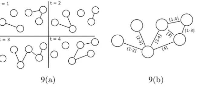
say the nodes u and v are neighbors in instant i. Note that we consider non directed edges. An example of an evolving graph can be found in Figure 1.

t = 1 t = 2

t = 3 t = 4

9(a) 9(b)

Figure 1: Figure1(a) shows 4 snapshots of the net-work’s connectivity and Figure 1(b) shows the cor-responding evolving graph.

A journey between two nodes u and v, noted J(u,v),

rep-resents the path built over time from u to v. Formally, J = (v0 t₁ → v1 t₂ → v2. . . vr−1 tr → vr), in which v0, v1, . . . , vr

are nodes in V (G), t1, t2, . . . , tr are time instants such that

t1 ≤ t2 ≤ . . . ≤ tr and (vi, vi+1) is an edge in E(Gi) for

every i between 0 and r − 1.

There are three different metrics in a journey and optimiz-ing each of them results in a different optimal journey.

Fore-mostjourneys are those optimizing message arrival time, or latency. Shortest journeys are those optimizing the number of edges, or hopcount. Fastest journeys are those optimiz-ing transit time, or the difference between arrival time and departure time.

3. SERVICES IMPLEMENTATION

In order to provide data about a dynamic network trace, we use the evolving graph model. By representing the net-work in this format, we get all the combinatorial base and existing algorithms this structure provides. This way, we can use these properties to extract information from the network so that it can be used in simulations.

To implement these analysis tools, we used the same evolv-ing graphs structure and code already used in some previous works [6, 7]. This program implements graphs as adjacency lists in which every edge is a list of intervals in which it is active and can be traversed. Using this format, it is pos-sible to work with arbitrary interval sizes (not necessarily integer). The system also implements the algorithms for op-timal journeys and facilitates the implementation of other functionalities.

To make these functionalities publicly available, a web system was implemented because this way, it is easily acces-sible by all the scientific comunity that works with dynamic networks, it does not require installation and facilitates data sharing. Nevertheless, the source code for the system will be available if anyone wants to install it in a local sever.

The DTNTES tool was developed in Java language, since the aforementioned evolving graphs structure is also

im-plemented is this language. The web framework used is

Google Web Toolkit, which allows the creation of efficient and portable web applications and allows the programmer to focus on the functionality rather than the adaptability to different browsers. This framework also provides the Google

Chart Tools, an API that creates and shows interactive and dynamic charts of various types in an easy and straigthfor-ward way. Figure 2 shows the system’s initial screen.

Figure 2: DTNTES system initial screen.

First of all, the user must upload his trace in one of the system’s supported formats. Then, the trace is interpreted and an evolving graph is built and saved for future use. The graph is stored in the system in a proper format, designed to facilitate parsing and interpretation. The file informs the number of nodes and the number of edges. For each edge, there is a line in the file with the two nodes, the time taken to traverse the edge and the list of intervals in which the edge is active. In this format, the graph is built edge by edge, eliminating the need to store any extra data.

The program data input accepts the format described above, and the ones accepted by the ONE simulator [8] and used in the DieselNet traces. Adding new formats is very simple and consists in the creation of a new reader class and adding it to the visual interface. Even though the system reads these different formats, the trace is always stored in the default format, since it is the most suited for the data recovery. The persistency is made with simple files, but can be easily extended to a database.

The functionality of the system consists in a set of services that can be executed over the traces. These services are split into connectivity related and journey related. In the next sections we detail the utility and implementation of every service in the DTNTES tool.

3.1 Connectivity services

The network connectivity is one of the most important aspects researchers must consider when choosing a trace for their work. The information about connectivity can radi-cally alter the interpretation of the results of a study de-veloped over a trace, since algorithms can have completely different behaviors depending on the frequency of the en-counters between nodes. For that reason, the main objec-tive of the tool is to provide information that allows the characterization of the density of the connections in a trace. To that end, the system provides five charts aggregat-ing information on connectivity: ratio of direct connections, ratio of journey connections, number of active direct con-nections over time, ratio of pairs connected by journeys over

(4)

time and stability index. The system also presents four met-rics to estimate the separation degree of the nodes in time and space. The metrics relative to the size of the journeys are very common in the study of complex networks [9]. The metrics related to the arrival date are equivalent to the space related, but adapted to the context of journeys. Those met-rics are the average and maximum foremost journey transit time and the average and maximum shortest journey size (also called diameter of the graph).

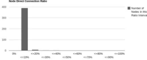
The direct connectivity ratio chart shows, for every node uin the graph, the size of the set of nodes S such that there is an edge (u, v) for every v in S divided by the total number of nodes. To calculate this set for a given node, this node’s adjacency list must be traversed and the number of edges on the list counted. The nodes have been grouped by ratio intervals so that a column chart can show the information more clearly.

With this chart, it is possible to visualize the degree of the nodes, if hub nodes exist (nodes that participate in many connections and, so, are very important for the network’s general connectivity) and it is possible to have an idea of the graph’s density, since if there are too many nodes with low direct connectivity ratio, then the graph is sparse. An example of this chart can be seen in Figure 3.

Figure 3: Exemple of a direct connectivity chart. To determine the graph’s connectivity by paths over time, the system provides a chart with the ratio of journey con-nections per node. For every node u, the ratio of nodes v in the graph to which exists a journey from u. Like in the previous chart, the data is grouped by ratio interval in a column chart. To calculate this number for one given node, the algorithm which calculates the foremost journey from this node to all the others in the graph is used. After exe-cuting this algorithm for every node, the number of journeys found for each node is counted.

With this chart, it is possible to visualize the reach of the nodes in terms of paths over time. Nodes that reach few others can deliver less messages than the ones which com-municate to many others by journeys. If most of the nodes have low reach, it means the graph is fragmented in small components. Otherwise, if many nodes have high journey connectivity, the graph has a large component containing most of the nodes. An example of this chart can be seen in Figure 4.

The previous two charts show the connection between nodes as a static property, which exists all the time the net-work is functioning, but it is not true. Connections, direct and by journeys, may fall after a short time, making the

Figure 4: Exemple of a journey connectivity chart.

numbers on the charts misleading. For that reason, the fol-lowing charts are very important, since they show the same data (number of direct and journey connections) over time. The number of active direct connections per time instant chart was calculated iterating over all the conections in the network and incrementing a connection counter for every time instant in its active interval. This chart shows the time periods in which connectivity increases or diminishes. High connectivity periods are more suitable for message de-livery or the execution of other distributed algorithms. Also, knowing the low connectivity periods may help energy sav-ing in mobile networks. An example of this chart can be seen in Figure 5.

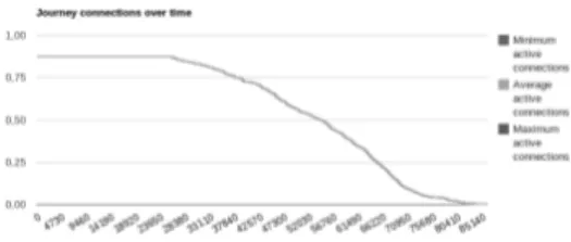
Figure 5: Exemple of an active connections chart. The journey connectivity per time instant chart was im-plemented using an algorithm derived from the foremost journey, which calculates the journey that leaves the origin node in the latest possible instant. This algorithm is called latest journey. We calculate this journey for every pair of nodes in the network and put their departure times in a list. When this list is sorted in decreasing order, the first time instant is the moment in which the last connection ends and so on. Thus, it is just a manner of counting the connections in each time interval using this list.

In this chart it is possible to visualize the decay of the network connectivity over time. The curve never rises be-caus if a journey exists in the future, it means any message generated before the journey’s latest departure date can be delivered. Therefore, in this curve, it is possible to identify the moments in which the connectivity falls permanently, as well as the overall network connectivity, which is the value observed at the beginning. This information is useful to

(5)

de-termine up to which moment the connectivity has a reliable ratio. An example of this chart can be seen in Figure 6.

Figure 6: Exemple of a journey connections chart.

To determine how important to the general network con-nectivity a single node is, the stability chart is used. The stability ratio of a node is defined as the difference between the number of pairs connected by journeys in the network when that node is removed and in the original network. This value points out the drop in the network connectivity that occurs if that node crashes. This metric is very useful to de-termine if there are hub nodes in the network and how many of them. An example of this chart can be seen in Figure 7

Figure 7: Exemple of a node stability chart.

In addition to the charts, the connectivity informations for every node in particular can be obtained in a text report, for computer processing or a different data aggregation. The report shows, for every node, every other node to which this one connects, the largest fully connected time and the last connection time.

3.2 Journey Services

The second class of services provided by the DTNTES is determining optimal journeys between pairs of nodes in every time instant. This information is useful in the devel-opment of routing protocols, since an algorithm generates a route between nodes which will hardly be optimal and the existence of a lower bound is extremely important. In most of the latest studies on this subject, the validation of a pro-tocol is done only through comparisons with other existing protocols. The problem in this approach is that every pro-tocol has bad cases, in which the results obtained are not good. The optimal journeys always provide the best results

possible, regardless of the case, which makes them a more trustworthy base of comparison.

The system allows the user to pick the origin and destina-tion nodes, shows the foremost journey, its arrival date, the shortest journey and its size. The journey display format shows the sequence of nodes, with the respective connec-tion instant between each pair. In case the journey is empty (when the origin and destination nodes are the same) or when there is no journey, a suitable message is displayed. The journey screen can be seen in Figure 8.

Figure 8: Exemple of the journey visualization screen.

In addition to this friendly interface, text reports with the full journeys, optimal arrival dates and sizes are available. The information on these reports are the same obtained through the visual interface, but grouped in text format to facilitate automatic processing.

The individual information on the optimal journeys in the network is useful when the user wishes to see a small num-ber of journeys quickly and in detail. In case many jour-neys are needed, the method loses eficiency. For this reason, the tool also provides the message log processing service. The user only has to upload a file containing, for each line, the origin node, destination node and message creation time and the system will return a report with the earliest arrival date and minimum hopcount for delivery of all the messages given. This service facilitates comparison between results of a routing protocol and the optimal results in a network and is especially important for researchers using traces in the study of routing algorithms.

3.3 Periodicity

Another aspect of dynamic networks approached by the DTNTES is the periodicity of the connections. We say an edge is periodic if there is a pattern in its connections and disconnections that repeats itself over time. If all the edges of a network are periodic, the network is periodic. This characteristic is important for many algorithms as it implies that every connection will repeat itself in the future, thus, the network connectivity over time never changes.

The problem of detecting a pattern in an edge’s connec-tions is similar to pattern searching in texts. But, since the searched pattern is not known, it is necessary to test all the possibilities, which takes quadratic time in the number of connections in the edge and the same calculation must be done for every edge in the network. The problem in this approach is that it only detects periodicity if the pattern is strictly followed, which will rarely be true in networks im-plemented in the real world. This way, the ideal would be to

(6)

find a definition of periodicity which allows a certain error margin so that an algorithm could get more useful results about the real traces.

The DTNTES provides a text report about the periodic-ity of each edge in the network, using the aforementioned strict approach. A slight modification allows the existance of a warmup period in the beginning before considering the periodicity. The report shows, for every edge, the size of the necessary warmup time and the size of every period of the edge, or a message in case the edge is not periodic. The usefulness of this information is limited due to the problems in the periodicity definition and it is a challenge to improve it and the algorithms to determine this property more accu-rately.

4. CASE STUDY: DIESELNET

To demonstrate the usefulness of the developed tool and all its functionalities, we will show, in this section, an ex-ample of its use with a real trace from the DieselNet [3] network. The goal of this study is to show what kind of information and conclusions are possible to extract from a trace using the DTNTES and how useful it can be to the field researchers.

DieselNet is a vehicular network infrastructure set on the University of Massachusetts Amherst campus, covering the neighboring county. It is made up of 30 buses equipped with HaCom Open Brick computers (577MHz CPU, 256Mb RAM) powered by a 24V battery. A 802.11b access point is connected to the computer and provides DHCP access to the passengers and passersby. A second 802.11b interface con-stantly scans the surrounding area in search of other buses and access points. Each bus runs Linux in a 40Gb HD and also carries a GPS that registers its position.

The traces used in this paper were obtained between Oc-tober 22nd _{and November 18}th_{, 2007, in work days only,}

making 20 days of traces. Each file constitutes a working day in the network and shows, for every connection between two buses or a bus and an external access point, one line containing the nodes’ identifiers, the time the connection begins, the duration in seconds, the amount of data trans-fered and the latitude and longitude of the connection. The files of bus to bus and bus to access point connections are separate but were merged before being inserted in the DT-NTES.

All the files from the 2007 DieselNet traces were uploaded to the tool so that a comparative analysis of the different days could be performed. In the next section, we show the results obtained from the DTNTES.

4.1 Characterizing the DieselNet network

First of all, we shall analyse the network metrics provided by the system in the information page. In Table 1, the data collected from all the days in the trace were aggregated. It is noticeable that the average transit time (difference be-tween the arrival and departure date) of a foremost journey between two nodes is almost 16000 seconds, almost 4 and a half hours. Considering there are a lot more access points than buses in the network, it is natural that the communi-cation between distant poins takes a long time, since it is necessary to wait for a vehicle to pass and take the message. The maximum transit time of a journey is practically 24h, which is the total working time of each file’s network.

By observing the shortest journey metrics it is noticeable

Metric Avg. Std. Deviation Avg. foremost. transit time 15909.6 1963.77 Max. foremost transit time. 85083.05 1183.35 Avg. shortest size 2.89 0.09 Max. shortest size 9.82 1.09

Table 1: Averages and standard deviations for the metrics of all the days of the DieselNet traces.

that the nodes are, in average, 3 hops apart. This implies that, in general, a message between two access points must pass through 2 buses to reach its destination. Since the time a shortest journeys takes to arrive is always bigger than a foremost journey, we can conclude that each hop takes over one and a half hour, in average. As shown by the standard deviations in the table, the network metrics generated by the many days are not so different, which can be explained by the fact that the buses have a fixed route and schedule.

In the direct connectivity and journey connectivity charts shown on Figures 9 and 10, it is noticeable that most of the nodes connect directly to less than 10% of the other nodes in the network, but, also, most of them connect by journeys to more than 90% of the nodes. This shows that the network has high connectivity by journeys, even though nearly all the nodes have low degree. From this data, we can infer that there is a large component in the graph, con-taining almost all the nodes and there may be smaller ones, but these constitute just a small fraction of network. The connectivity charts are very similar for all the days in the trace, presenting the same distributions of number of nodes per ratio interval.

Figure 9: Number of nodes per direct connectivity ratio interval chart for one of the DieselNet days.

Figure 10: Number of nodes per journey connectiv-ity ratio interval chart for one of the DieselNet days.

In the direct active connections per time instant chart, we can see that there is a large period of time with no connec-tivity, approximately between the 9000 and 22000 seconds (between 2h30 and 6h in the morning) in all the days of the

(7)

trace. With this information we can infer that the buses do not circulate during the early hours, so, this period could be ignored by the users of the trace, or used as a warmup time for the algorithms. The number of direct active connections is somewhat constant during the daytime, falling a little in the night. In some days, the no connection period is larger, starting before 1h, which shows that some days the bus run until later. Apart from this minor difference, the traces are very similar in all the days. The Figure 11 shows the chart for one of the days.

Figure 11: Number of direct active connections per time instant chart for one of the DieselNet days.

In the journey connections over time chart, we can notice that the connectivity starts at approximately 85% and keeps this level during all the night, since no connections are lost in this period. During the day, the connectivity ratio drops gradually, which is natural, considering many of the bus to access point connections probably happen only once a day. The fact that there are no sudden connectivity drops points to the absence of bridge connections (those that, if lost, divide the graph in two components).

Figure 12: Ratio of pairs of nodes communicating by journeys per time instant chart for one the Diesel-Net days.

The connectivity curves are very simular in all of the days, each one reaching less than 50% approximately at 50000 onds (14h) and less than 25% approximately at 65000 sec-onds (18h). The curves also show a concavity shift between the 50% and 25% connectivity, which indicates a steeper drop in this point and slower drop near the end of the work-ing time. Figure 12 shows this chart for one of the days.

In the stability chart, we can see that practically all the nodes cause less than 10% of disconnection on the network if removed. This is true for all the days in the trace, with some of them having 1 or 2 nodes causing between 10% and 20% of disconnection. This fact shows that the DieselNet traces are very stable and not vulnerable to single crashes. It is natural that the crash of an external access point should not affect the overall connectivity, but it is expected that if a bus stops working, many pairs of access points would disconnect. But, as the chart in Figure 13 shows, a single bus crash does not cause a significant loss of connectivity.

Figure 13: Number of nodes per stability index in-terval for one of the DieselNet days.

5. CONCLUSION

In this work, we presented the Delay Tolerant Network Trace Evaluator System, described the implementation of all its connectivity and journey services and showed an example of its utilization by studying the DieselNet network trace. The system is available in the page

http://grenoble.ime.usp.br/∼paulo/dtn/dtntes.

We believe this tool will be very useful for researchers who wish to extract information about a trace before using it or to reach more precise conclusions about their studies. In the same way, the data about journeys and message delivery is very useful to provide a lower bound for routing protocols.

As future work, new functionalities can be added to the system to improve data visualization, raise the amount of information provided, the number of accepted formats for trace upload, among other upgrades in user interface. Fur-thermore, it is a challenge to improve the definition of pe-riodicity in order to provide useful tools to determine that property on the traces.

6. REFERENCES

[1] “Umass trace repository,” http://traces.cs.umass.edu/, accessed in January 2012.

[2] “Crawdad - a community resource for archiving wireless data at dartmouth,” http://crawdad.cs.dartmouth.edu, accessed in January 2012.

[3] A. Balasubramanian, B. Levine, and A. Venkataramani, “Enhancing interactive web applications in hybrid

networks,” in 14th MobiCom. ACM, 2008, pp. 70–80. [4] J. Burgess, B. Gallagher, D. Jensen, and B. Levine,

“Maxprop: Routing for vehicle-based

disruption-tolerant networks,” in Proc. IEEE InfoCom, vol. 6. Barcelona, Spain, 2006, pp. 1–11.

[5] A. Ferreira, “On models and algorithms for dynamic communication networks: The case for evolving graphs,” in 4o

AlgoTel, 2002, pp. 155–161.

[6] A. Goldman, P. Floriano, and C. Machado, “Optimal journeys and trade-offs on dtns,” in 2nd ExtremeCom, 2010.

[7] A. Goldman, C. Ferreira, C. Machado, and P. Floriano, “Jornadas mais r´apidas e compromissos em DTNs,” in

XXVIII SBRC, 2010.

[8] A. Keränen, J. Ott, and T. Kärkkäinen, “The ONE Simulator for DTN Protocol Evaluation,” in SIMUTools

’09: Proceedings of the 2nd ICST. New York, NY, USA: ICST, 2009.

[9] A. Loureiro, A. Frery, R. Mini, A. Aquino, H. Ramos, and M. Almiron, “Redes complexas na modelagem de redes de computadores,” SBRC 2010 Minicursos, 2010.