HAL Id: hal-01886649
https://hal.archives-ouvertes.fr/hal-01886649v2
Submitted on 18 Mar 2019
HAL is a multi-disciplinary open access
archive for the deposit and dissemination of
sci-entific research documents, whether they are
pub-lished or not. The documents may come from
teaching and research institutions in France or
abroad, or from public or private research centers.
L’archive ouverte pluridisciplinaire HAL, est
destinée au dépôt et à la diffusion de documents
scientifiques de niveau recherche, publiés ou non,
émanant des établissements d’enseignement et de
recherche français ou étrangers, des laboratoires
publics ou privés.
An intuitive approach to structuring the three
polarization components of light
F. Maucher, Stefan Skupin, S. A. Gardiner, I. G. Hughes
To cite this version:
F. Maucher, Stefan Skupin, S. A. Gardiner, I. G. Hughes. An intuitive approach to structuring the
three polarization components of light. New Journal of Physics, Institute of Physics: Open Access
Journals, 2019, 21 (1), pp.013032. �10.1088/1367-2630/aaf711�. �hal-01886649v2�
PAPER • OPEN ACCESS
An intuitive approach to structuring the three electric field components of
light
To cite this article: F Maucher et al 2019 New J. Phys. 21 013032
View the article online for updates and enhancements.
New J. Phys. 21(2019) 013032 https://doi.org/10.1088/1367-2630/aaf711
PAPER
An intuitive approach to structuring the three electric
field
components of light
F Maucher1,2,3
, S Skupin4
, S A Gardiner2
and I G Hughes2
1 Department of Physics and Astronomy, Aarhus University, Ny Munkegade 120, DK-8000 Aarhus C, Denmark
2 Joint Quantum Centre(JQC) Durham-Newcastle, Department of Physics, Durham University, Durham DH1 3LE, United Kingdom 3 Department of Mathematical Sciences, Durham University, Durham DH1 3LE, United Kingdom
4 Univ.Lyon, Université Claude Bernard Lyon 1, CNRS, Institut Lumière Matière, F-69622, Villeurbanne, France
E-mail:[email protected]
Keywords: electromagnetic optics, laser beam shaping, optical vortices, tighly focused beams
Abstract
This paper presents intuitive interpretations of tightly focused beams of light by drawing analogies
with two-dimensional electrostatics, magnetostatics and
fluid dynamics. We use a Helmholtz
decomposition of the transverse electric
field components in the transverse plane to introduce
generalized radial and azimuthal polarization states. This reveals the interplay between transverse and
longitudinal electric
field components in a transparent fashion. Our approach yields a comprehensive
understanding of tightly focused laser beams, which we illustrate through several insightful examples.
1. Introduction
Unless the beam’s transverse electric field components are divergence-free in the two-dimensional transverse plane[1], tightly focused light typically leads to a non-negligible longitudinal electric field component [2,3],
where the terms longitudinal and transverse electricfield components refer to the components of the electric field that are parallel or perpendicular, respectively, to the direction of the mean Poynting flux. Having a longitudinal electricfield component does not add a new degree of freedom, in the sense that all components of the electric and magneticfields are still fixed by prescribing two components in a plane. However, it is the electric field component parallel to the direction of the Poynting flux, and that makes it somewhat special. Taking the longitudinal electricfield component properly into account leads to a range of novel physical phenomena, such as a significant decrease of the focal spot size [4,5], the realization of so-called ‘needle beams’ [6] and Möbius
strips in the polarization of light[7]. In the context of light-matter interaction, taking into account the effect of
the longitudinal electricfield component can be crucial [8], and it may even dominate over the transverse
components[9].
While the longitudinal electricfield component and its interplay with the transverse components has attracted significant interest over the last two decades [3,10,11,12], the discussion has usually been limited to
special cases assuming certain spatial symmetries, and a simple and general intuitive picture would be highly desirable. This paper aims to provide such a picture, and presents a novel approach towards an intuitive understanding of tightly focused beams by making analogies withfluid dynamics and with two-dimensional magneto- and electrostatics. For this, a two-dimensional Helmholtz decomposition of the transverse electric field components in the transverse plane [1] is key. The Helmholtz decomposition allows the generalization of
the notion of‘radial’ and ‘azimuthal’ polarization in the following way: radial polarization corresponds to an electricfield that is ‘curl-free’ in the transverse plane—which as we shall see can be interpreted as a flow solely due to sinks and sources without vorticity—and is the part of the field that gives rise to the longitudinal
polarization. An azimuthally polarized electricfield is ‘divergence-free’ in the transverse plane—analogous with a flow solely due to vorticity without any sinks or sources—and does not give rise to any longitudinal electric field component. Employing those polarization states turns out to be very useful for computing numerically exact solutions to Maxwell’s equations with structured electric field components, and moreover facilitates an intuitive understanding of tightly focused vector beams.
OPEN ACCESS RECEIVED
11 November 2018
REVISED
1 December 2018
ACCEPTED FOR PUBLICATION
7 December 2018
PUBLISHED
30 January 2019
Original content from this work may be used under the terms of theCreative Commons Attribution 3.0 licence.
Any further distribution of this work must maintain attribution to the author(s) and the title of the work, journal citation and DOI.
The paper is organized as follows. In section2we introduce the nomenclature, present the equations of motion, and detail the connection between radially and azimuthally polarizedfields, and curl- and divergence-free solutions in the transverse plane. In section3we draw analogies with electrostatics, magnetostatics andfluid dynamics, hence presenting intuitive interpretations offields that are ‘divergence-free’ and ‘curl-free’ in the transverse plane. Finally, in section4we present several intuitive examples to illustrate the analogies and convey an appreciation of the concept of generalized radial and azimuthal polarization states. Starting with basic Laguerre–Gaussian (LG) modes, we show constructions of complex random and topological beams.
2. Model
The three electricfield components of a tightly focused monochromatic beam (frequency ω, wavelength λ=2π c/ω, vacuum light velocity c) in free space are described by
2E r(^,z)+k02E r(^,z)=0, ( )1 ·E r(^,z)= ^·E^+ ¶z zE =0. ( )2 We have introducedk02=w2 c2= (2p l)2, the transverse coordinatesr^=(x y, ), and the transverse electric field components E⊥=(Ex, Ey). In what follows, we consider the wavelength λ to be a fixed scaling parameter to
equation(1). Note that E represents the complex amplitude vector of the beam; the full electric field has an
additional trivial time-dependenceexp(-iwt)that is omitted here.
For a given amplitude vector in the focal plane5Ef(r⊥)=E(r⊥, z=0), the propagation in the positive z direction can be easily computed in the transverse spatial Fourier domain as
=
^ ^ ^
ˆ ( z) ˆ ( ) ( ) ( )
E k , E kf eikzk z, 3
wherekz( )k^ = k02-k^2 and k⊥=(kx, ky); the symbolˆdenotes the Fourier transform with respect to r⊥. It
is important to note that Efcannot be arbitrarily prescribed in all three components. We use a two-dimensional Helmholtz decomposition to depict the most general expression for the two transverse components, as[1]
= - ¶ ¶ + -¶ ¶ ^ ^ ^ ^ ^ ^ ⎛ ⎝ ⎜ ⎞ ⎠ ⎟ ⎛ ⎝ ⎜ ⎞ ⎠ ⎟
(
)
( ) ( ) ( ) ( ) ( ) ( ) V V W W E r r r r r 0 1 1 0 , 4 x y x y fwhereV( )r^ andW( )r^ denote arbitrary(sufficiently well behaved) scalar potentials. The first term, which we
denoteE^f,V = -^V, corresponds to afield that is curl-free in the transverse two-dimensional plane, that is,
´^ E^f,V =0. The second term we denoteEf,^W = ¶( yW,-¶xW), which gives rise to a divergence-freefield in
the transverse two-dimensional plane,6that is, ^·E^f,W =0. The longitudinal electricfield component Ezis
therefore coupled solely toE^f,V, and together with the potential V it obeys a Poisson equation
D^V( )r^ = ¶z z z 0E∣= ( )r .^ ( )5
Because the z dependence of Ezis known from equation(3), Ezfcan be readily obtained in Fourier space from
-k^2Vˆ ( )k^ =ikz(k^) ˆ (Ez k^). ( )6 f
For given potentials V and W the full solution can therefore be written in transverse Fourier space as
= + -^ ^ ^ ^ ^ ^ ⎡ ⎣ ⎢ ⎢ ⎢ ⎢ ⎛ ⎝ ⎜ ⎜ ⎜ ⎜ ⎞ ⎠ ⎟ ⎟ ⎟ ⎟ ⎛ ⎝ ⎜ ⎜ ⎞ ⎠ ⎟ ⎟ ⎤ ⎦ ⎥ ⎥ ⎥ ⎥ ˆ ( ) ( ) ˆ ( ) ˆ ( ) ( ) ( ) z k k k V k k W E k k k k k , i 0 e . 7 x y z y x k k z 2 iz
Hence, the potential V generates the electricfield EV, the three vector components of which are in general nonzero. By way of contrast, the potential W generates the electricfield EW, the longitudinal component of which vanishes(EzW=0). For reasons which become clear in section4.1we will call EVradially polarized, and EWazimuthally polarized. Other polarization states imply certain conditions on the potentials V and W: transverse linear polarization, withα Ex=(1−α) Eywith 0α1, requires
a - -a ^ = a + -a ^
[ kx (1 )k Vy] ˆ (k ) [ ky (1 )k Wx] ˆ (k ); ( )8
5
Any other z=constant plane could also be used.
6
The electricfield in vacuum always fulfills·E=0. Hence, the restriction‘in the transverse two-dimensional plane’ is crucial in the present context.
and transverse circular polarization, with Ex=±iEy, requires
=
^ ^
ˆ ( ) ˆ ( ) ( )
V k iW k . 9
These definitions do not involve the longitudinal component Ez, which is why they are termed transverse. From
equations(8) and (9), the well-known fact that any nonzero linearly or circularly polarized field necessarily gives
rise to a longitudinal electricfield component becomes immediately clear; in these cases V is nonzero and has a nontrivial spatial dependence, and hence equation(5) gives rise to a nonzero Ez. Throughout this paper, we will
refer to these transverse polarization states when we mention linear and circular polarization. We note, however, that in the definitions for linear and circular polarization involving all three electric field components (see, e.g. [11]) both cases would be elliptically polarized.
Before we consider analogies and interpretations of the expressions found, we would like to connect our approach to the respective literature. The generating potentials for tightly focused vector beams were formulated in[11,13]: given a scalar solution Ψ to the scalar Helmholtz equation, we can write down the transverse
magnetic polarizedfield (TM polarization) as µ ¶ Y -¶ YB ( y , x , 0), and the associated electricfield reads µ ¶ ¶ Y ¶ ¶ Y -¶ Y - ¶ Y( )
E x z , y z , x2 2y . Hence, a TM beam corresponds to afield E V
with V∝ ∂zΨ in our
nomenclature. The transverse electric polarizedfield (TE polarization) can be readily obtained via the dual transformationE cB andB - cE , corresponding to afield EWwith W∝ Ψ in our nomenclature. However, the notations TM and TE polarization are usually used in the context of two-dimensional systems with translational invariance in one direction(Fresnel reflection, waveguides, etc.), and thus we do not adopt them here. Moreover, this paper focuses primarily on the electricfield E and henceforth we will not discuss the magneticfield B. An experimental visualization of the structures presented in this work would entail some form of atom-light interactions, and it is well known that the electricfield dominates the magnetic field when interacting with charges in a medium(see, e.g. [14]).
3. Interpretations and analogies
Let us now interpret the equations from the last section and lay out analogies with two-dimensional electro- and magnetostatics andfluid dynamics.
3.1. Curl-freefields produced by potential V
Wefirst consider fields EVthat are curl-free in the transverse plane, that is,fields obtained when W=0. The aim is to understand how the transverse electricfield componentsE^f,Vrelate to the longitudinal component Ezf.
Equation(5) represents a Poisson equation in two dimensions for the potential V(x, y), the solution of which in
transverse Fourier space is given by equation(6). The source term for this Poisson equation is given by ¶z z z 0E∣= ,
which depends on the transverse coordinates r⊥only.
The source term ¶z z z 0E∣= involves the longitudinal derivative, and not the component Ezfdirectly. However,
making use of equation(3) in transverse Fourier space we can approximate the source term to lowest order as
¶ = ^ = ^ ^ » ^ + ^ ⎛ ⎝ ⎜ ⎞ ⎠ ⎟ ˆ ∣ ( ) ( ) ˆ ( ) ˆ ( ) ( ) E k E k E k k i k k i k k , 10 z z z 0 z z z f 0 f 2 02
thereby disposing of this derivative term. Equation(10) is of course only a rough estimate, with an error that
grows with the degree of the light’s non-paraxiality. It nevertheless gives an idea of the qualitative behavior of Ezf,
as will be illustrated in section4.
To see the analogy with two-dimensional electrostatics, we must simply identify -¶z z z 0E∣= with a charge
densityρ(x, y). The transverse electric field componentsE^f,Vthen follow from the same equations as the two-dimensional electrostaticfieldE^s(x y, ), as summarized in table1.
There is, however, a subtlety related to this analogy requiring comment. The opticalfield amplitude E is complex-valued, and the full electricfield has a temporal dependence that is hidden in this representation, unlike the two-dimensional electrostaticfield which is real-valued and time-independent. Thus, in general, we must separate the real and imaginary parts of E and solve two‘electrostatic’ problems.
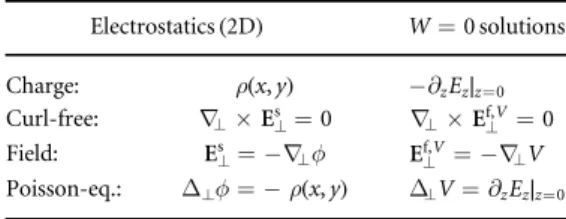
Table 1. Analogy with electrostatics in two dimensions.
Electrostatics(2D) W=0 solutions Charge: ρ(x, y) -¶z z z 0E∣= Curl-free: ´^ E^s =0 ´^ E^f,V=0 Field: E^s = -^f E^f,V = -^V Poisson-eq.: Δ⊥f=−ρ(x, y) D^V= ¶z z z 0E∣= 3
3.2. Divergence-freefields produced by potential W
Here we are interested in solutions EWthat are divergence-free in the transverse plane(V = 0, and consequently =
EzW 0). The potential W can be interpreted as the longitudinal component of a vector potential, that is, = ´We
E W
z
f, . Then, by taking the curl of this equation, we get
D^W( )r^ = ¶y xEf( )r^ - ¶x yEf( )r ,^ (11) a Poisson equation for the potential W.
This leads to a straightforward analogy with magnetostatics7. If we identify the potential W with the only nonzero componentAzsof a magnetic vector potential
=
^ ^
( ) ( ) ( )
As r Azs r ez, 12
the induced static magneticfieldBs= ´Ascan be associated with Ef,W. The static current density follows
from ´Bs=m J
0 s, andflows perpendicular to the (x,y) plane under consideration. Hence, Jzsis the only
nonzero component, and corresponds to the negative source term in equation(11). The complete magnetostatic
analogy is summarized in table2.
A similar remark as given above concerning the complex-valued opticalfield amplitude applies, in that two real-valued magnetostatic problems may need to be solved to describe one curl-free opticalfield. Furthermore, it is important to note that this represents a formal analogy only; the analog magneticfieldBsmust not be confused
with the magneticfield B of the vector beam (see also the discussion at the very end of section2).
3.3. Fields produced by both potentialsV and W
In the most general situation, both potentials V and W are nonzero. In this case the opticalfield
= +
Ef Ef,V Ef,Whas a perfect analogy influid dynamics [15]. For a fluid with density ñ and flow velocity field
u, conservation of mass dictates the continuity equation
¶t (r,t)+ · [ (r,t) (u r,t)]=0. (13) We consider a layer of thisfluid in a z=constant plane, e.g. z=0, with in- and outflow ñuzinto the layer. We
denote theflow velocity field in this layeru rl( )^ =u r ,(^ z=0). In the stationary situation(∂tñ=0), and
furthermore assuming homogenity and incompressibility(∇ñ=0), we find that
^·u r^ ^l( )= -¶z z zu∣=0( )r .^ (14)
Equation(14) is identical to equation (2) if we identifyu^l with ^ Ef, and we write = + ^ ^ ^ ul ul,cf ul,df, where ^ ul,cfis
curl-free in the z=0 plane ( ´^ u^l,cf =0), andu^l,dfdivergence-free(^·u^l,df =0).
The analogy betweenu^l,cfand Ef,Vfollows immediately: the curl-free velocityfieldu^l,cfcan be written as the
negative gradient of the so-called velocity potentialf, and the spatial in- and outflow rate ¶z z z 0u∣= acts as a
source term in the Poisson equation for the velocity potential, as shown in table3.
Following[15], let us now turn towards the divergence-free (two-dimensional) velocity fieldu^l,df, which
obeys the continuity equation
¶x xul,df( )r^ + ¶y yul,df( )r^ =0. (15) This implies that the differential y =d uxl,dfdy-uyl,dfdxis exact, and the scalar stream functionψ can be found (up to a constant) as line integral from some reference point to a given point
ò
ò
y( ) -y( )= dy= uxl,dfdy-uyl,dfd .x (16) In particular any integration curve joining the two points yields the same result8. Influid dynamics, the stream function characterizes theflow velocity quite intuitively, as already suggested by its name. The ‘flux’ across aTable 2. Analogy with magnetostatics in two dimensions.
Magnetostatics withJs=J rzs( )^ez V=0 solutions Current: m0Jzs= ¶x yBs- ¶y xBs ¶x yEf- ¶y xEf Div.-free: ^·B^s =0 ^·E^f,W=0 Field: B^s = ¶( yAzs,-¶xAzs) E^f,W= ¶( yW,-¶xW) Poisson-eq.: D^Azs= -m0Jzs D^W= ¶y xEf- ¶x yEf
7
We follow the common terminology which labels magneticfields of stationary currents as magnetostatic, even though time inversion symmetry is violated.
8
closed curve, that is, =, is zero. Since the‘flux’ across any curve joining the two pointsand depends only on the values ofψ at these two points, it is clear that ψ is constant along a streamline.
Influid dynamics, one commonly defines the vorticity as
w = ´u^l = ¶( x yul- ¶y xul)ez= Wez. (17) The vorticity vector is oriented perpendicular to our plane of interest, and its nonzero componentΩ, together with the stream functionψ, obeys a Poisson equation:
y
D^ ( )r^ = -W( )r .^ (18) Hence,E^f,Wcan be interpreted as the divergence-free velocityfieldu^l,dfof a two-dimensional incompressible
fluid, which is composed of vortices only and does not contain sources or sinks. The potential W must be associated with thefluid stream function ψ determined by the longitudinal component Ω of the vorticity w. The full analogy is summarized in table4.
In summary, we note that two-dimensional incompressiblefluid dynamics permits coverage of the cases of both curl- and divergence-freefields (V = 0 and W = 0, respectively), as shown in tables3and4, and thus represents a unified analogy. One must bear in mind, however, that in fluid dynamics the flow velocity field u is real valued, and so in general twofluid problems are necessary to represent one complex optical field.
4. Examples
We now present several intuitive examples to illustrate ourfindings, highlighting the concept of generalized radial and azimuthal polarization, and exploiting the aforementioned analogies to construct numerically exact vector beams.
There are two general remarks to be made before prescribing any potential orfield components. Firstly, the relevant quantities must not contain any evanescent amplitudes, that is, in the transverse Fourier domaink all^
fields and potentials must be zero fork^2 k02. Otherwise, equation(3) gives an exponentially growing solution
for negative z, which renders it unphysical in the bulk. Therefore, in the examples that follow we systematically apply thefilter function
l = - - < ^ ^ ^ ^ ⎧ ⎨ ⎪⎪ ⎩ ⎪ ⎪ ⎡ ⎣ ⎢ ⎢ ⎤ ⎦ ⎥ ⎥ ( )k ( k ) k ( ) k H k k k exp 1 2 for 0 for 19 k 2 2 0 2 2 02 2 02 0
to these quantities. Secondly, equation(2) implies thatE kˆ (z ^=0)=0 f
for solutions propagating in the z direction. This is automatically fulfilled when Ezf(or ¶z z z 0E∣= ) is computed from a given potential V. However, if Ezf(or 
=
∣
E
z z z 0) is prescribed, special care must be taken. A suitable filter function is then
= - l ^ - ^ ( )k ( ) ( ) H 1 e k , 20 0 3 2
which we have applied in the examples below when needed.
Table 4. Analogy with divergence-free velocityfield flow. Fluid dynamics(2D) V=0 solutions Vorticity: W = ¶x yul- ¶y xul ¶x yEf- ¶y xEf Div.-free: ^·u^l,df=0 ^·E^f,W=0 Field: u^l,df= ¶( yy,-¶xy) Ef,^W= ¶( yW,-¶xW) Poisson-eq.: D = -Wy DW= ¶y xEf- ¶x yEf
Table 3. Analogy with curl-free velocityfield flow.
Fluid dynamics(2D) W=0 solutions Sources and sinks: ¶z z z 0u∣= ¶z z z 0E∣= Curl-free: ´^ u^l,cf=0 ´^ E^f, V=0 Field: u^l,cf= -^f = - ^ ^V Ef, V Poisson-eq.: D^f= ¶z z z 0u∣= D^V= ¶z z z 0E∣= 5
4.1. Radial and azimuthal polarization
Let usfirst consider the simplest examples of bell-shaped V and W potentials, producing classic radially and azimuthally polarized vector beams, respectively. In terms of LG profiles, we therefore takeLGs00( )r^, that is, a
simple Gaussian,fixing its width to σ=λ/2. As explained above, we must filter the potentials in the transverse Fourier domain by multiplying them by Hk0in order to remove evanescent waves.
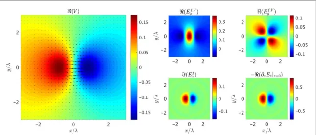
4.1.1. Gaussian‘electrostatic potential’ V
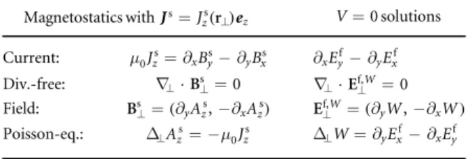
Given that we use the constraint W=0, and V is chosen to be a real-valued function, we require only the real parts ofE^f,Vand ¶z z z 0E∣= , and the imaginary part of Ezf. We therefore depict these components only infigure1,
which displays the resulting radially polarized beam. It follows straightforwardly that we get two dipole-like light distributions in the transverse electricfield components from such a bell-shaped ‘electrostatic potential’ V. Going further with this analogy, the‘charge density’-¶z z z 0E∣= µ(1-2r^2 l2)exp(-2r^2 l2)inducing such a
potential consists of a positive hump and a negative ring. The shape of this‘charge density’ is very close to the longitudinal component Ezf, which justifies the estimation given by equation (10).
4.1.2. Gaussian‘magnetic vector potential’ W
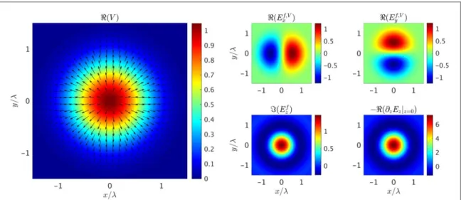
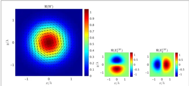
In order to produce an azimuthally polarized vector beam, we simply let W be the real-valued Gaussian, and set V=0. Figure2shows that the vectorfieldE^f,Wis tangential to the contour lines of W. This is exactly what one
would expect from the magnetostatic analogy, where W corresponds to the longitudinal componentAzsof the magnetic vector potential. We do not depict the static current density Jzsthat would generate such a vector potential and respective magnetostaticfield. However, its profile has exactly the same form as the ‘charge density’ -¶z z z 0E∣= infigure1: a positive bell-shaped current density at the center, surrounded by a negative
ring-like return current.
4.1.3. Circularly polarized vortex beam
In section2, we discussed how to choose the potentials V and W such that the transversefields are circularly polarized, namely iW=V. Hence, complex superposition of thefields shown in figures1and2should give a circularly polarized beam. Infigure3we display the resulting transversefield components ExfandEyf, which are
indeed two singly charged vortices. The corresponding longitudinal electricfield component Ezfis not shown, because it is the same as that shown infigure1.
This rather straightforward construction of circularly polarized beams works for any pair of generalized radially and azimuthally polarized beams with±iW=V. The motivation for this consideration stems from the fact that in such an arrangement one has a beam that is both linearly(the longitudinal electric field component) as well as circularly polarized(the transverse polarization components). This could play an important role for imprinting structures onto matter, since the longitudinal electricfield component could drive a different transition to the transverse electricfield components.
Figure 1. A real-valued Gaussian potentialVµexp(-2r^2 l2)produces a radially polarized beam. The transverse electricfieldE^f,Vis indicated by arrows. The inducedfield components and the ‘charge density’ -¶z z z 0E∣= are shown on the right.
4.2. Longitudinal vortex beam
Let us now use our previousfindings to construct a beam featuring a singly charged vortex in its longitudinal component Ezf. Because such a vortex is composed of two orthogonal dipoles in the real and imaginary parts, we may start with a dipole. Moreover, we want to make use of thefluid dynamics analogy, and prescribe a real-valued dipole in the‘spatial in- and outflow rate,’¶z z z 0E∣= µx exp(-2r^2 l2). The induced velocity potential is
easily obtained in the transverse Fourier domain as
fˆ µH k expk x (-lk^ 8) k^, (21)
dipole 2 2 2
0
where we apply thefilter function Hk0to remove any evanescent waves. The resulting potential in position space
is shown infigure4, together with all electricfield components. In terms of the fluid dynamics analogy, where we interpret the transversefield as the flow velocity, a very intuitive picture arises: peak and trough of the dipole in ¶z z z 0E∣= act like source and sink for the‘flow.’ With the approximation equation (10), even the longitudinal
component Ezfby itself can be identified with the source of the ‘transverse flow.’
In principle, we can now construct a beam with the desired singly charged vortex in its longitudinal component by employing the potentialV x y( , )=fdipole(x y, )ifdipole(y x, ), that is, by addingfdipole
rotated by±π/2 as the imaginary part of V. The resulting beam is radially polarized in the generalized sense
Figure 2. A real-valued Gaussian potentialWµexp(-2r^2 l2)produces an azimuthally polarized beam. The purely transverse electricfieldE^f,Wis indicated by arrows. The inducedfield components are shown on the right ( =E 0
zf ).
Figure 3. Transversefield components of a circularly polarized single charge vortex beam produced by complex superposition of figures1and2, that is,V=iWµexp(-2r^2 l2).
7
introduced earlier, because W=0. It is, however, not the easiest realization of a longitudinal vortex, as we will see below.
The transverse electricfield components Exf,VandEyf,Vshown infigure4appear to be relatively intricate, and so the natural question arises whether it is possible to simplify the‘transverse flow’ by adding a divergence-free velocityfield through an appropriate stream function ψ. The main flow is clearly in the positive x direction, and so we may choose the stream functionψ such that the y component of the total flow velocity is zero. Equation (8)
tells us that yˆ = -kyfˆ kx
dipole
will suffice, which translates into y(x y, )= -fdipole(y x, )in position space. And indeed,figure5confirms thatEyf,W = -Eyf,V, that is, the total‘transverse flow’ is parallel to ex.
Hence, the potentialsV x y( , )=fdipole(x y, )ifdipole(y x, )andW x y( , )= -fdipole(y x, )
f (x y)
i dipole , produce a longitudinal vortex as well, but with much simpler transversefield components. Figure6 shows the resulting opticalfields (for the + sign), and it even turns out that transverse components are bell-shaped. Moreover, the transversefield is circularly polarized, as W=iV. We have therefore constructed the solution reported in[16], where a longitudinal vortex was achieved by tightly focusing a circularly polarized
bell-shaped light distribution.
It is important to note that the choice of the‘stream function’ W is the degree of freedom one has when only the longitudinal electricfield component is prescribed. In the present example, we used W to simplify the transverse electricfield components. In section4.4, we will demonstrate that W can be used as well to engineer certain topological properties of the transversefields.
Figure 4. A real-valued dipole is prescribed in ¶z z z 0E∣=, and the resulting potentialV=fdipole(see text for details) is used to compute the electricfield components.
Figure 5. The real-valued potentialW x y( , )= -fdipole(y x, )(see text for details) producesE = -E
4.3. Random beam
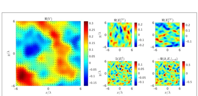
Let us prescribe a rather complicated longitudinalfield component Ezf—a random beam, as shown in figure7.
For this case, we simply consider a super-Gaussian beam profile inEzf, exp(-r10 (10l) )10 , and multiply the
latter with complex random numbers at each point of the numerical grid. The complex-valued random numbers are constructed asf=x1exp 2 i( p x2), with real-valued random numbers x1,2Î [0, 1]. The resulting beam profile is then multiplied in transverse Fourier space by both filter functions Hk0and H0, as introduced
above. In order to facilitate comparison with previousfigures, we choose to show ( )I Ezf , such that all other
derived quantities infigure7are real valued. Furthermore, we plot only the center part of the beam.
We now make several important remarks regardingfigure7. First of all, the‘charge density’ -¶z z z 0E∣= , to
once more take the electrostatic analogy, features a pattern very close to that prescribed in (I Ezf). This means that even here the approximation equation(10) yields insight, and the longitudinal component Ezfcan be
identified directly as a ‘charge density.’ Moreover, figure7shows very nicely how the landscape of the ‘electrostatic potential’R V( )induced by (I Ezf)‘shapes’ the transverse electric field components
^
( ) R Ef,V . In
contrast to the previous examples, the peaks and troughs of (I Ezf)cannot be directly related to the peaks and troughs ofR V( ). This can be understood by thinking of V as being a convolution between the Green’s function of the two-dimensional Poisson equation(which is long-ranged) and the ‘charge density’: the convolution
Figure 6. A bell-shaped circularly polarized transversefield produces a singly charged vortex inEzf. The off-axis signflips in the phase plot are due to thefilter function Hk0(see text).
Figure 7. A random profile is prescribed inI E( zf)(see text for details). The real-valued ‘charge density’ -¶z z z 0E∣= looks very similar. Corresponding potential V and transversefield components are shown as well.
9
cannot resolve the delicate structure of the source term and simply smears it out. This also explains why the structures in the transversefield components are larger than those in Ezf.
4.4. Linked trefoils in transverse and longitudinal components
We discussed the remaining degrees of freedom whenfixing the longitudinal electric field component Ezfin
section4.2, where they were exploited to simplify the transverse profiles. In principle, nothing prevents us from prescribing twofield components, say EzfandEyf, in the focal plane. This allows us to engineer both transverse and longitudinal components, and the potentials V and W determine the complete opticalfield via equation (7).
Here, we will demonstrate the tremendous possibilities of creating customized vector beams by creating knotted vortex lines in the longitudinal and one transverse electricfield component (Ey). Apart from optics,
knotted and linked vortex lines have also recently been studied in a range of different contexts, such as classical fluid dynamics [17], excitable media [18–21], nematic colloids [22–24] and superfluids such as Bose–Einstein
condensates[25,26]. In the present context, optical vortex knots [1,27,28] can be used to imprint topological
light structures onto the latter[29,30].
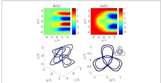
The topology of the two knots we envisage is sketched infigure8: the vortex lines of the Eyand Ez
components form two linked trefoil knots. To create such a vector beam, the respective components can be prescribed in the focal plane as
= s - s + s - s - s ( )
Eyf 5LG00y 7LG01y 40LG02y 18LG03y 30LG ,30y 22
= s - s + s - s - s ( )
Ezf 8LG00z 18LG01z 40LG02z 18LG03z 34LG ,30z 23 withσy=0.42λ and σz=0.5λ. The formulas of equation (23) were obtained according to [27,30], with
coefficients adapted to the non-paraxial situation [1]. We filter in transverse Fourier space with Hk0and H0,
where the latter is only necessary for Ezf.
Even though atfirst glance the two linked vortex knots in figure8may seem somewhat contrived, they highlight that vortex lines in different electricfield components can be chosen to be arbitrarily close without reconnecting. This is not possible for vortex lines in a single electricfield component, which could be of importance when considering inscribing these vortex lines onto matter. Furthermore, such a topology demonstrates the tremendous possibilities of structured light.
The transverse electricfield component Exfis fully determined by equation(23). Even though EzfandEyf
havefinite support, Exfis nonzero on a semi-infinite interval and thus impractical (see figure8). Such
semi-infinite field components occur when at least one of the other components integrated over the respective variable does not vanish: in our case,Eˆy z, (kx=0,ky)¹0
f
. Nevertheless, this problem of impracticalfield components can be circumvented by simply attenuating the beam with, e.g. a sufficiently wide super-Gaussian profile, without affecting the propagation of the components of interest close to the optical axis. Additional satellite spots will appear far from the axis, but we have checked that for a super-Gaussianexp[-r10^ (10l) ]10
those spots do not interfere with the linked vortex knots.
Figure 8. Two linked trefoils in different components of the electricfield: the blue line represents the vortex line in Ey, the black line the vortex line in Ez. The corresponding(semi-infinite) profiles inExfare shown in the upper panels.
5. Conclusions
In this paper we have presented a systematic route to construct numerically exact vector beams. By means of a Helmholtz decomposition of the transverse electricfield components in a plane transverse to the optical axis, we show that the full electromagneticfield can be generated by two scalar potentials V and W. The potential V produces‘curl-free’ (in the transverse plane) fields with a nonzero longitudinal component. The potential W produces‘divergence-free’ (in the transverse plane) fields with zero longitudinal component. We suggest naming these generalized radial and azimuthal polarization states, respectively. The decomposition of the optical field into generalized radial (W = 0) and azimuthal (V = 0) polarization states allows us to draw several analogies with other physical systems, that is, electrostatics, magnetostatics, andfluid dynamics. By means of these analogies, it is possible develop an intuitive understanding of the interrelation between longitudinal and transverse electricfield components, and the scalar potentials assume a ‘physical meaning’. Finally, we presented several examples to illustrate the proposed decomposition and analogies. Besides rather simple configurations such as longitudinal vortices, we demonstrated arbitrary random beams as well as sophisticated topological light configurations. In all these examples, the above analogies were used to explain features in the respective electric field components, or even to conceive the beam configurations.
We believe that ourfindings will broaden the range of accessible vector beams extensively and trigger further theoretical and experimental investigations involving structured light.
Funding Information
This work is funded by the Leverhulme Trust Research Programme Grant RP2013-K-009, SPOCK: Scientific Properties Of Complex Knots. SS acknowledges support by the Qatar National Research Fund through the National Priorities Research Program(Grant No. NPRP 8-246-1-060).
ORCID iDs
F Maucher https://orcid.org/0000-0002-5808-3967 S Skupin https://orcid.org/0000-0002-9215-1150 S A Gardiner https://orcid.org/0000-0001-5939-4612 I G Hughes https://orcid.org/0000-0001-6322-6435References
[1] Maucher F, Skupin S, Gardiner S A and Hughes I G 2018 Creating complex optical longitudinal polarization structures Phys. Rev. Lett.
120 163903
[2] Richards B and Wolf E 1959 Electromagnetic diffraction in optical systems. ii. structure of the image field in an aplanatic system Proc. R. Soc. A253 358–79
[3] Youngworth K S and Brown T G 2000 Focusing of high numerical aperture cylindrical-vector beams Opt. Express7 77
[4] Quabis S, Dorn R, Eberler M, Glöckl O and Leuchs G 2000 Focusing light to a tighter spot Opt. Commun.179 7
[5] Dorn R, Quabis S and Leuchs G 2003 Sharper focus for a radially polarized light beam Phys. Rev. Lett.91 233901
[6] Wang H, Shi L, Lukyanchuk B, Sheppard C and Chong C T 2008 Creation of a needle of longitudinally polarized light in vacuum using binary optics Nat. Photon.2 501
[7] Bauer T, Banzer P, Karimi E, Orlov S, Rubano A, Marrucci L, Santamato E, Boyd R W and Leuchs G 2015 Observation of optical polarization Möbius strips Science347 964–6
[8] Quinteiro G F, Schmidt-Kaler F and Schmiegelow C T 2017 Twisted-light-ion interaction: the role of longitudinal fields Phys. Rev. Lett.
119 253203
[9] Hnatovsky C, Shvedov V, Krolikowski W and Rode A 2011 Revealing local field structure of focused ultrashort pulses Phys. Rev. Lett.
106 123901
[10] Nye J F 1999 Natural Focusing and Fine Structure of Light: Caustics and Wave Dislocations (Bristol: Institute of Physics Publishing) [11] Lekner J 2003 Polarization of tightly focused laser beams J. Opt. A: Pure Appl. Opt.5 6
[12] Otte E, Tekce K and Denz C 2017 Tailored intensity landscapes by tight focusing of singular vector beams Opt. Express25 20194–201
[13] Lekner J 2016 Tight focusing of light beams: a set of exact solutions Proc. R. Soc. A472 20160538
[14] Adams C S and Hughes I G 2018 Optics f2f (Oxford: Oxford University Press)
[15] Batchelor G K 2000 An Introduction to Fluid Dynamics (Cambridge: Cambridge University Press)
[16] Nieminen T A, Stilgoe A B, Heckenberg N R and Rubinsztein-Dunlop H 2008 Angular momentum of a strongly focused Gaussian beam J. Opt. A: Pure Appl. Opt.10 115005
[17] Kleckner D and Irvine W T M 2013 Creation and dynamics of knotted vortices Nat. Phys.9 253
[18] Maucher F and Sutcliffe P M 2016 Untangling knots via reaction-diffusion dynamics of vortex strings Phys. Rev. Lett.116 178101
[19] Maucher F and Sutcliffe P M 2017 Length of excitable knots Phys. Rev. E96 012218
[20] Maucher F and Sutcliffe P M 2018 Dynamics of linked filaments in excitable media arXiv:1804.07064
[21] Binysh J, Whitfield C A and Alexander G P 2019 Stable and unstable vortex knots in excitable media Phys. Rev. E99 012211
[22] Tkalec U, Ravnik M, Copar S, Zumer S and Musevic I 2011 Reconfigurable knots and links in chiral nematic colloids Science333 62–5
11
[23] Martinez A, Ravnik M, Lucero B, Visvanathan R, Zumer S and Smalyukh I I 2014 Mutually tangled colloidal knots and induced defect loops in nematicfields Nat. Mater.13 258–63
[24] Martinez A, Hermosillo L, Tasinkevych M and Smalyukh I I 2015 Linked topological colloids in a nematic host Proc. Natl Acad. Sci. USA112 4546–51
[25] Proment D, Onorato M and Barenghi C F 2012 Vortex knots in a Bose–Einstein condensate Phys. Rev. E85 036306
[26] Kleckner D, Kauffman L H and Irvine W T M 2016 How superfluid vortex knots untie Nat. Phys.12 650
[27] Dennis M R, King R P, Jack B, O’Holleran K and Padgett M J 2010 Isolated optical vortex knots Nat. Phys.6 121
[28] Sugic D and Dennis M R 2018 Singular knot bundle in light J. Opt. Soc. Am. A35 1987–99
[29] Ruostekoski J and Dutton Z 2005 Engineering vortex rings and systems for controlled studies of vortex interactions in Bose-Einstein condensates Phys. Rev. A72 063626