Convolutional Embedding of Attributed Molecular
Graphs for Physical Property Prediction
The MIT Faculty has made this article openly available.
Please share
how this access benefits you. Your story matters.
Citation
Coley, Connor W. et al “Convolutional Embedding of Attributed
Molecular Graphs for Physical Property Prediction.” Journal of
Chemical Information and Modeling 57, 8 (July 2017): 1757–1772 ©
2017 American Chemical Society
As Published
http://dx.doi.org/10.1021/acs.jcim.6b00601
Publisher
American Chemical Society (ACS)
Version
Author's final manuscript
Citable link
http://hdl.handle.net/1721.1/116837
Terms of Use
Article is made available in accordance with the publisher's
policy and may be subject to US copyright law. Please refer to the
publisher's site for terms of use.
Connor W. Coleya, Regina Barzilayb, William H. Greena, Tommi S. Jaakkolab, Klavs F. Jensena†
a Department of Chemical Engineering, Massachusetts Institute of Technology; 77 Massachusetts Avenue, Cambridge, MA 02139
b Computer Science and Artificial Intelligence Laboratory, Massachusetts Institute of Technology; 77 Massachusetts Avenue, Cambridge, MA 02139
† Corresponding author
Abstract. The task of learning an expressive molecular representation is central to developing quantitative structure-activity and property relationships. Traditional approaches rely on group additivity rules, empirical measurements or parameters, or generation of thousands of descriptors. In this paper, we employ a convolutional neural network for this embedding task by treating molecules as undirected graphs with attributed nodes and edges. Simple atom and bond attributes are used to construct atom-specific feature vectors that take into account the local chemical environment using different neighborhood radii. By working directly with the full molecular graph, there is a greater opportunity for models to identify important features relevant to a prediction task. Unlike other graph-based approaches, our atom featurization preserves molecule-level spatial information that significantly enhances model performance. Our models learn to identify important features of atom clusters for the prediction of aqueous solubility, octanol solubility, melting point, and toxicity. Extensions and limitations of this strategy are discussed.
Introduction
The accurate prediction of chemical properties or activities from molecular structures is a topic of significant interest in the chemical community.1 Common prediction targets include performance in a biological assay, mutagenicity, solubility, and octanol-water partitioning (mimicking tissue-blood partitioning). If these properties can be accurately predicted, experimental high-throughput screening (HTS) can be supplemented or replaced by virtual HTS.2 Predictive models can assist in lead optimization and in determining whether drug candidates should proceed to later development stages. This utility extends to chemical synthesis, particularly in flow chemistry, for the prediction of solubilities to anticipate solids formation, vapor pressures to anticipate gas evolution, and perhaps eventually, rates and yields of chemical reactions using solvation corrections to quantum chemistry estimates of transition states.
For decades, the development of reliable quantitative activity-structure or property-structure relationships (QSAR or QSPR, often used interchangeably) has been an area of active research for in silico prediction of properties directly from molecular structures. Briefly, the idea is to take a molecule, , extract a suite of structural or chemical features to construct a feature vector, , and predict the final property based on that information, . There are a few common approaches to molecular feature extraction, , including the following:
(i) Generation of sparse bit vectors with indices corresponding to the presence or absence of molecular substructures. Traditional fingerprints using a limited set of predefined substructures have developed into extended connectivity
the molecular representation. The importance of any one substructure over another is not presupposed, but multiple substructures are represented by the same fingerprint index.
(ii) Determination of empirical solute descriptors. Linear free energy relationships are examples of this approach.4 In the case of Abraham relationships, each solute is described by five empirical parameters, corresponding to different chemical functionalities; solvents are similarly parameterized. The free energy of solvation or any derivative property is then written as a combination of solute-solvent interactions.
(iii) Concatenation of many known molecular descriptors, which may include calculation of electronic descriptors or the use of existing property-estimation models. There are many software packages designed to calculate hundreds or even thousands of descriptors, including Dragon5 and CDK6 among others. The majority of recent QSAR studies rely on this approach.
(iv) Less commonly, SMILES strings or InChI strings, which are two different methods to encode molecules as a character sequence can be directly used directly as model inputs.7-10
As expected, initial approaches to the second half of the prediction task, , involved simple regressions (e.g., linear, quadratic)11; due to the high dimensionality of feature vectors, individual features with little effect on the final prediction are often downselected to produce a lower-dimensional, less-parameterized regression.1, 12 These regression techniques progressed into more advanced techniques as machine learning grew in popularity, including the use of support vector machines, random forest models, Bayesian networks, and artificial neural networks. The application of machine learning to QSAR regression problems has been the subject of several studies and reviews.13-17
Despite the application of machine learning approaches to , insufficient attention has been paid to developing flexible approaches to the first step – the embedding strategy that produces a molecular feature vector. This step may offer more room for improvement than the regression technique alone. Multiple important substructures can “collide” into the same fingerprint index in an ECFP3, while other indices may be irrelevant to the prediction task, because there is no flexibility in index assignment. Empirical descriptors either require experimental data, a prohibitive requirement for virtual high throughput screening, or a separate QSPR model to predict those descriptors. Descriptor-based models rely on the assumption that all information relevant to the prediction task is included in the chosen descriptor set, limiting the opportunity for a model to learn beyond current chemical expertise.
Learning a proper molecular representation, , while learning its relation to the prediction target, , can lead to superior performance over fixed-representation models. Lusci and Baldi describe recurrent neural network models that treat molecules as sets of undirected, acyclic graphs after performing suitable disconnections.18 Duvenaud et al. reported a convolutional neural network as a differentiable (i.e., trainable) alternative to circular
fingerprints.19 More recently, Kearnes et al. reported an alternate graph convolution approach for prediction of outcomes in various biological assays.20 Each of these three approaches use only simple structural attributes calculable based on the immediate neighborhood around an atom with the exception of Kearnes et al., who include an estimate of partial charge. Because the only spatial information available is graph distance, information more closely related to 3D geometric distances (e.g., whether an atom is exposed enough to participate in solute-solvent interactions) is lost. The authors would
like to note that since the submission of this manuscript, a number of studies have explored similar ideas of flexible molecular representation.21-25
In this paper, we describe a convolutional neural network model related to the work of Duvenaud et al. that resembles a learned Morgan circular fingerprint. Our approach combines the flexibility offered by convolutional networks with a more information-rich featurization enabled by work in descriptor-based models. The parameterized representation function and the parameterized regression function are trained simultaneously, so that the representation can adapt to capture what is needed for the prediction task. By including atom-level features calculated over the entire molecule, rather than using purely local atomic features, we demonstrate a substantial improvement in model predictive performance for four property targets: octanol solubility, aqueous solubility, melting point, and biological toxicity.
Methods
Model design
Our model begins by representing each molecule as an undirected graph containing nodes (atoms) with features and edges (bonds) with features . Atom feature vectors are iteratively updated based on those calculated at the previous depth. The neighboring atom vectors are combined linearly with associated bond vectors and passed through a non-linear activation function to obtain new atom vectors. We turn atom feature vectors into longer atom fingerprint vectors via another learned mapping so that the resulting fingerprint vectors can be simply summed to get the molecular fingerprint at the current depth. That resulting fingerprint representation is passed through additional hidden layers in a feed forward neural network to yield a single scalar value, e.g. octanol solubility in log10(M) or a Boolean prediction, e.g. activity in a bioassay.
The initial attribute vectors of each atom, “depth-0” atom feature vectors, are passed through a shared hidden layer with softmax activation to build depth-0 atom fingerprints, which are summed to form a depth-0 molecular fingerprint. Depth-1 atom feature vectors are calculated from each atom’s depth-0 atom feature vector and information about its neighbors. Neighboring atoms’ depth-0 atom feature vectors concatenated with their respective connecting bonds’ features to form atom-bond feature vectors. Neighboring atom-bond feature vectors are passed through a hidden neural network layer and summed to form the new depth-1 atom features. Bond attributes are not updated and thus persist throughout this convolution process. These depth-1 atom feature vectors are passed through a shared output layer to build depth-1 atom fingerprints, which are summed to form a depth-1 molecular fingerprint.
This process is repeated up to a specified maximum depth. At different depths, different network weights are used. All depth- molecular fingerprints are summed to form the overall molecular fingerprint. An expanded description of this algorithm can be found in the Supporting Information (Section S1). The output of the embedding step is a learned fingerprint. This fingerprint is fully connected to a single hidden neural network layer with tanh activation, in turn fully connected to a single output node with linear or sigmoid activation. The full workflow is shown schematically in Figure 1.
Figure 1. Model architecture using a graph-based convolutional neural network for molecular embedding.
Initial representation
One of the attractive features of this convolutional embedding strategy is that the model should be able to use very simple atom and bond descriptors and still learn a proper feature vector representation of an atom and its neighborhood. Due to the similarity between this approach and ECFPs, similar structural attributes are used here. To preserve spatial and other molecular information beyond connectivity, a set of attributes are calculated at the molecular-level as a sum of atom-level contributions; these atom-level contributions are explicitly included in our featurization. RDKit26, an open-source cheminformatics package, was used for SMILES27 string parsing and attribute calculations. These are shown in Table 1 and Table 2. Discrete variables are encoded as “one-hot” vectors with a length equal to the number of choices and a single non-zero entry at the index corresponding to the position of the variable’s value in the set of choices.
Table 1. Atom features Fi included in initial representation. adenotes features calculated at the molecular level, which are excluded from certain representative models for comparative purposes.
Indices Description
0 - 10 Atomic identity as a one-hot vector of B, N, C, O, F, P, S, Cl, Br, I, other
11-16 Number of heavy neighbors as one-hot vector of 0, 1, 2, 3, 4, 5 17-21 Number of hydrogens as one-hot vector of 0, 1, 2, 3, 4 22 Formal charge
23 Is in a ring 24 Is aromatic 25a Crippen contribution to logP
26 a Crippen contribution to Molar Refractivity 27 a Total Polar Surface Area contribution 28a Labute Approximate Surface Area contribution 29 a Estate index
30 a Gasteiger partial charge 31 a Gasteiger hydrogen partial charge
Indices Description
0-3 Bond order as one-hot vector of 1, 1.5, 2, 3 4 Is aromatic
5 Is conjugated 6 Is in a ring
7 Placeholder, is a bond
Implementation approach
All models are implemented in Python using the machine learning library Keras28 built on Theano.29, 30 The use of autodifferentiation packages greatly accelerates neural network training by pre-compiling the computational graph required to update parameters during training. For each molecule, we define a molecular tensor ∈
⋅ ⋅ where is the combined number of atom and bond features, such that
,
, 0
, , connected 0, 0 otherwise
∀ , ∈ 1, …
The final index along the third dimension of is merely a flag to denote the presence of a bond and, accordingly, the subtensor slice , , is the adjacency matrix. In fact, the 3D molecular tensor can be thought of as a 2D adjacency matrix extended in a third dimension to incorporate atom and bond features. As a simple example of this tensor
representation, take ethanol and the alternate set of attributes shown in Figure 2. Using the atomic number, number of hydrogens, and formal charge as atom features and the bond order, aromaticity, conjugation, ring status, and a placeholder 1 as bond features, the molecular tensor for ethanol can be represented by piecing together the representations of each atom and bond according to the above equation.
Figure 2. Extraction of simple atom and bond attributes for ethanol. Atoms and bonds are individually color coded to indicate how their features are used to populate the molecular tensor, .
The size of the molecular tensor, ( ⋅ ⋅ ), is much larger than is strictly necessary to store all of the relevant information. In this implementation, for ease of integration with Keras, molecular graphs are reduced to a
multi-tensor representation. In this manner, any molecule of arbitrary size and arbitrary connectivity can be embedded using the same pre-optimized tensor operations. For each molecule, three tensors are defined as the adjacency matrix , an atom-feature matrix , and a bond-feature matrix .
∈ ⋅
∈ ⋅⋅
∈ ⋅
Parameters and hyperparameters
The model is able to learn a suitable molecular embedding from data due to the flexibility enabled by its
parametrization. Atom feature vectors are updated by multiplying the neighboring atom-bond feature vectors by a learned weight matrix and passing the result through a non-linear activation function. A unique weight matrix is used at each depth so the model learns a distinct update procedure for earlier updates (small-neighborhood features) and later updates (large-neighborhood features). Similarly, the weights used to map atom feature vectors to longer atom fingerprints are learned during training and are also unique to each depth. The two weight matrices that map the final molecular fingerprint to the hidden layer and the hidden layer to the output are also learned.
This architecture possesses numerous hyperparameters: the length of the fingerprint; the length (and featurization) of the atom and bond attributes; the internal feature vector activation function; the output activation function; the
maximum radius or depth to incorporate contributions from; the number of nodes in the hidden layer; the hidden layer activation function. As with any network, the dropout probabilities at each layer and the learning rate and/or training schedule can also be tuned. In unreported tests, including dropout did not tend to improve test set performance, as dropout and similar regularization techniques are more suitable for dense, fully-connected layers. The grid used for
hyperparameter searching was defined from depths {2, 3, 4, 5}, inner atom-level representation sizes {32, 64, 128}, and learning rates {0.003, 0.001, 0.0003, 0.0001, 0.00003}. Empirically, performance was most sensitive to the learning rate.
Datasets
We selected datasets which are publically available and have been used for property prediction tasks previously. There is one representative dataset each from octanol solubility, aqueous solubility, and melting point. The existence of duplicate entries in these datasets that are commonly used for benchmarking can defeat the purpose of a cross-validation study, where the training and testing datasets are meant to be fully disjoint.31, 32 Values corresponding to duplicate entries, as recognized by having identical isomeric SMILES strings, are averaged. The exact datasets used in this study, before and after processing, can be found in the Supporting Information (Section S4).
1. Abraham octanol solubility dataset consisting of 282 molecules and their corresponding solubilities in
log10(mol/L).33 A large portion of this dataset came from an earlier paper by Admire and Yakowlsky.34 Of these 282, only 255 chemical names could be unambiguously converted to their structure using the Chemical Identifier Resolver35 so the remaining 27 were excluded from this study. An additional 10 pairs in their table were found to be duplicated entries, so
these were averaged to avoid redundancies. The final dataset contains 245 compounds and their octanol solubilities. All values are reported with units of log10(mol/L).
2. Delaney small aqueous solubility dataset consisting of 1144 small molecules and their corresponding intrinsic solubilities in log10(mol/L).11 The dataset of 2874 molecules was split in the original paper to three sets of “small” ( 1144), “medium” ( 485), and “large” ( 1245). We use the label “Delaney” to refer to this small set only. After averaging out duplicates, we are left with 1116 molecules. All values are reported with units of log10(mol/L).
3. Bradley double plus good, or “Bradley good” melting point dataset of 3,041 measurements36; this is a pre-curated subset of the larger Bradley dataset37. After averaging duplicates and filtering molecules which could not be parsed automatically by RDKit (e.g., due to implicit hydrogens on aromatic nitrogen), a final dataset of 3,019 molecules was obtained. Note that this is not identical to the dataset used by Tetko et al.38, 39, which contains only 2,878 compounds and excludes the 155 that also appear in the Bergstrom dataset.40 All values are reported with units of degrees Celsius.
4. Tox21 dataset containing binary (active/inactive) toxicity data for thousands of compounds on 12 targets, originally released as part of the Toxicology in the 21st Century Data Challenge 2014.41 The Tox21 training set contains 6069-8982 inactive and 301098 active compounds for each assay; the leaderboard set contains 186-289 inactive and 3-48 active compounds for each; the evaluation data contains 647 additional compounds. The training and leaderboard sets are used to evaluate single-task model performance using an internal ECFP baseline. Multitask models are trained on a dataset combining the training and leaderboard examples and tested using the larger evaluation dataset, consistent with the original Tox21 challenge. Among the many entries for this competition, we focus our comparison on Mayr et al.’s
DeepTox, which won the competition’s grand challenge by demonstrating the highest performance of all methods.42
Testing procedure – Abraham, Delaney, Bradley datasets
We select performance measures which enable the most accurate comparison to existing models as well as provide a conservative estimate of model generalizability (i.e., overestimate prediction error for new molecules). The exact datasets used are available in the Supporting Information to encourage comparison.
A 5-fold CV, standard in QSAR evaluation13, was run in triplicate was used for the three datasets. For consistency in prediction to literature models, a randomized CV was used in lieu of more structured time-split43 or cluster CV.32, 44 Use of a structure-based cluster CV would result in quantitatively different performance values. Within each fold, the training data (80%) was randomly split 4:1 (64%:16%) into a true training set and an internal validation set. The internal
validation set was used to screen hyperparameter settings for each fold using a broad, pre-defined grid search31, 45 in addition to indicating when to stop training using an additional hyperparameter, the patience, . A consensus model weighted by performance on the internal validation data set was used to make the final predictions on the 20% test data in each CV fold. To minimize the influence of the random 4:1 internal validation split on performance, the internal
validation was run in triplicate. Training stopped once there had been 10 consecutive epochs without reducing the validation set error or once the maximum number of epochs was reached. In practice, was set to be large enough that the training was always terminated by early stopping.
The use of consensus models can inhibit model interpretability, as each individual model will be slightly different. For the sake of interpretability and discussion, we also include a set of models where hyperparameters were fixed in advance of training. These hyperparameter settings and learning schedules are described in Table S1.
Comparison of machine learning models to empirical regression models is inherently challenging. Few-parameter regressions, like Abraham linear free energy relationships, are often performed on the entire dataset and the entire dataset is subsequently used to evaluate the goodness of fit; techniques such as leave-one-out cross validation (LOOCV) are used to estimate the prediction error of the theoretical next prediction. However, all methods should be evaluated using data not already used in training or fitting. This is particularly true for a highly-parameterized model such as a neural network, as there are often enough degrees of freedom that it is possible to reach nearly zero error on the training dataset. The training data used to estimate model weights must be completely separate from the testing data used to evaluate performance.
We evaluate performance for scalar predictions using four common metrics based on model residuals, : the mean-squared error (MSE), the mean absolute error (MAE), the standard deviation of residuals (SD), and the closely related root mean-squared error (RMSE).
, , 1 1 | | 1 1 ̅ √
In addition to literature comparisons, we also establish baseline performance metrics using support vector machines (SVMs) similarly trained and tested using a randomized 5-fold CV (Section S3). Molecules are represented by fixed length ECFP4 or ECFP6 fingerprints ( 512, to match the learned fingerprint length). Three kernel functions were tested: a linear kernel, a radial basis function kernel, and a Tanimoto similarity score kernel.
Testing procedure – Tox21 dataset
The explicit partitioning of the Tox21 dataset into training compounds and testing compounds enables a more straightforward method of model evaluation: performance on the test set. As with the physical property models, the training data was randomly split 4:1 into a true training set and an internal validation set. The internal validation set was used to screen hyperparameter settings for each fold using the same broad, pre-defined grid search. A consensus model weighted by performance on the internal validation data set was used to make the final predictions. We evaluate the
Boolean activity predictions using the Area Under the Receiver Operating Characteristic curve (AUROC, or AUC) as implemented in scikit-learn46. This metric represents the area under the step function when the true positive rate is plotted against the false positive rate.47
Results
Octanol solubility
Admire and Yakowlsky analyze the use of the general solubility equation (GSE) for predicting the octanol solubility of small molecule compounds34. Using a dataset of 223 compounds, they report a standard deviation of residuals (SD) of 0.71 using the following equation:
log 0.50 0.01 m. p. 25
where the melting point (m.p.) is measured in degrees Celsius. They found this expression more reliable for compounds which are miscible with octanol at room temperature in their liquid state than those which are immiscible; for many compounds, the room temperature liquid state is the hypothetical supercooled liquid. This expression requires knowing only the compound’s melting point – a single experimental value.
Abraham and Acree build on this idea by incorporating melting point as an additional input to one form of Abraham’s linear free energy relationship expressions33. Because their models require knowing solute descriptors (in this case, four descriptors), only 201 measurements from Admire and Yakowlsky’s data are used to obtain an SD of 0.61 without experimental melting points and 0.47 with experimental melting points. They expand the dataset to 282 molecules and calculate a SD of 0.63 and 0.47 for the following two models:
0.604 0.942 0.311 0.588 0.463 0.540 1.104 ∗
0.480 0.355 0.203 1.521 0.408 0.364 1.294 ∗ 0.00813 . . 25 Superior performance to the GSE is expected based on the additional information required for each solute, i.e. requiring empirical solute parameters in place of or in addition to melting points.
Because this is a small dataset ( 245), one might not expect strong performance from a neural network model; there are very few training examples with which to learn how to generalize. Performance for the consensus model and model with typical hyperparameters are shown in Table 3. An example loss (MSE) curve plot during training is shown for the representataive model in Figure 3. The validation dataset consists of only 20 samples and understandably exhibits a very noisy loss profile during training, which makes it difficult to use for early stopping. While a larger internal validation set would alleviate this issue, it would also decrease the amount of data used for actual training.
Table 3. 5-fold CV performance on the Abraham octanol solubility dataset, averaged over three runs. Original units are log10(mol/L).
Model Required data Number
of samples
MSE MAE SD
Best SVM baseline - 245b 0.467 0.019 0.520 0.008 0.680 0.013
GSE 34 Melting point 223 0.71
Abraham and Acree, m.p. 33 Four empirical descriptors
& melting point 282
a 0.47
CNN-Ab-oct-representative[*] - 245b 0.413 0.018 0.496 0.014 0.641 0.011
CNN-Ab-oct-representative - 245b 0.338 0.005 0.455 0.007 0.581 0.005
CNN-Ab-oct-consensus - 245b 0.328 0.022 0.455 0.015 0.573 0.019
a201 from ref. 34, 81 additional;, b all 245 from ref. 33, with 37 unparseable or duplicated removed; [*]molecular calculations were excluded from the initial atom featurization.
Figure 3. Representative loss curves during 5-fold CV training for a single CNN model with typical hyperparameters. The small size of the internal validation dataset (20 molecules) results in a very noisy loss profile, decreasing the reliability of its use for hyperparameter selection or early
stopping during training.
Within the Abraham octanol dataset, certain compounds are consistently harder to predict than others. In Figure 4, the histogram of residuals is shown for one run of the representative model. The highly non-normal shape suggests that the overall performance metrics are strongly affected by outliers. The molecules corresponding to the most under- and over-predicted octanol solubilties in this data set are shown in Figure 5. Of particular note are PCB 194 (1,2,3,4-tetrachloro-5-(2,3,4,5-tetrachlorophenyl)benzene) and PCB 209
(1,2,3,4,5-pentachloro-6-(2,3,4,5,6-pentachlorophenyl)benzene), two extreme outliers on opposite sides of the spectrum. Although the recorded solubilities are quite different, they are structurally very similar and thus the model predicts values close to their average; this is true also of the consensus model.
Figure 4. Prediction residuals for the representative Abraham octanol solubility model; skewness = -0.33, kurtosis = 3.42.
Figure 5. Molecules from the Abraham octanol dataset with solubilities that are most significantly (a) under-predicted and (b) over-predicted by one run of the representative model. Captions are experimental solubility (residual of prediction) [log10(M)].
Aqueous solubility
In his original paper, Delaney constructed a regression model starting with 9 molecular descriptors including clogP, an estimate of the octanol/water partition coefficient.11 Performance on the “small” dataset of 1144 compounds is reported in terms of MAE for his regression model (0.75) and the GSE requiring experimental melting point (0.47). Despite having a larger error, the regression model does not require knowledge of solute melting points.
Lusci et al. implement a recursive neural network treating molecules as acyclic graphs or undirected graphs.18 Using a 10-fold CV with internal consensus modeling, they report a best-case RMSE of 0.58±0.07 and a MAE of 0.43 log molar units on the Delaney dataset with 1144 (i.e., duplicates were not removed). Duvenaud et al. also used the Delaney dataset for benchmarking in a 5-fold CV and report a best-case mean predictive accuracy of 0.52 log10 molar units.19
Results using the modified small Delaney dataset of 1,116 compounds are shown for various hyperparameter settings in Table 4. The molecules with the most under- and over-predicted solubilities from the representative CNN-De-aq-representative with moelcular features are shown in Figure 6.
Table 4. 5-fold CV performance on the Delaney aqueous solubility dataset, averaged over three runs. Original units are log10(mol/L).
Model Number of samples MSE MAE SD
Best SVM baseline 1116a 1.255 0.011 0.821 0.006 1.117 0.004 Lusci et al. 18 1144 0.34 0.43 Duvenaud et al. 19 1144 0.52 CNN-De-aq-representative[*] 1116a 0.334 0.011 0.424 0.005 0.577 0.010 CNN-De-aq-representative 1116a 0.312 0.003 0.401 0.002 0.559 0.003 CNN-De-aq-consensus 1116a 0.314 0.008 0.403 0.005 0.560 0.007
a1116 from ref. 11, duplicates removed; [*]molecular calculations were excluded from the initial atom featurization.
Figure 6. Molecules from the Delaney aqueous dataset with solubilities that are most significantly (a) under-predicted and (b) over-predicted by one run of the representative model. Captions are experimental solubility (residual) [log10(M)].
Melting point
Two studies by Tetko et al.39 test models on the Bradley good dataset (save the 155 from the Bergstrom set) and report a best-case RMSE of 32.2 degrees. The model that obtained this figure was trained on a dataset of 289,394 measurements combining five datasets including the Bradley good dataset itself. A consensus model trained on the incomplete Bradley good dataset using a 5-fold CV is reported to have a RSME of 34.6 degrees. As inputs to their models before downselection, Tetko et al. use a total of eleven descriptor packages including four 3D packages: CDK, Dragon, Chemaxon, and Adriana.Code.38
Performance of the convolutional models are shown in Table 5. For this prediction task, the model of Tetko et al. 39 is slightly superior to the convolutional models; this is explained by their use of numerous descriptor calculations, which perhaps capture structural or electronic attributes of the molecule more fully than the convolutional model can with the limited number of training samples and only simple atom-level descriptors. Significant outliers from the representative model are shown in Figure 7.
Table 5. 5-fold CV performance on Bradley good melting point dataset, averaged over three runs. Original units are degrees Celsius.
Model Number of samples MSE MAE SD
Best SVM baseline 3019b 3330 28 43.26 0.28 57.21 0.25
Tetko et al.39 2878a 1197
CNN-Br-tm-representative[*] 3019b 1421 23 27.55 0.15 37.69 0.29
CNN-Br-tm-representative 3019b 1337 13 26.59 0.14 36.51 0.16
CNN-Br-tm-consensus 3019b 1264 24 26.18 0.30 35.54 0.33
a2878 from ref. 36, 155 removed that overlapped with ref. 40 b3019 from ref. 36, unparseable and duplicates removed; [*]molecular
calculations were excluded from the initial atom featurization.
Figure 7. Molecules from the Bradley dataset with melting points that are (a) under-predicted and (b) over-predicted by one run of the representative model. Captions are experimental melting point (residual) [degrees Celsius].
Pre-training and multitask physical property results
The previous section demonstrated model performance when weights were learned, from scratch, for each prediction target independently. During training, the embedding layer begins to incorporate the relevant attributed substructures into the feature vector as it learns how to represent a molecule.
To probe the universality of the learned embeddings, a model was trained using the Delaney representative hyperparameters on the entire small Delaney dataset (i.e., not in a cross validation). The weights from the trained model are then used to initialize a second model to predict octanol solubilities in a 5-fold CV using the Abraham dataset; only the weights between the hidden layer and dense output layer are reset, so the new model begins with the same fingerprint representation. The results of this cross-initialization, the reverse case, and an octanol solubility model initialized with the learned Bradley melting point fingerprint are shown in Table 6.
Model Prediction MSE MAE SD
CNN-De-aq-all-Ab-oct-representative oct 0.328 0.015 0.446 0.008 0.571 0.011
CNN-Br-tm-all-Ab-oct-representative oct 0.424 0.007 0.501 0.001 0.651 0.005
Table 6. 5-fold CV performance for various models, with weights initialized by training a model on the entirety of the other dataset using the previously-found representative model, averaged over three runs. Original units are log10(M).
The standalone aqueous model (CNN-De-aq-representative) performs slightly better than the cross-initialized model (CNN-Ab-oct-all-De-aq-representative); there is a larger, albeit still small, improvement in the aqueous-initialized octanol model (CNN-De-aq-all-Ab-oct-representative) over the standalone (CNN-Ab-oct-representative), from a SD of 0.581 0.005 to 0.571 0.011. These improvements suggest a commonality between the features important for aqueous and octanol solubilities. This is consistent with other approaches; for example, Abraham parameterizes solutes with the same 5 empirical descriptors regardless of solvent choice and standard group additivity approaches similarly subdivide molecules using a fixed set of functional groups or substructures. With the Delaney and Abraham datasets in particular, it makes sense that the smaller dataset (Abraham, 245) would benefit more significantly from initialization with the learned weights of the larger dataset (Delaney, 1116), than vice versa.
Based on the reasonable performance of the GSE in predicting octanol solubility, demonstrated by Admire and Yakowlsky34, one might expect that initialization of an octanol model with weights of a melting point model would be preferred to an aqueous model. The opposite trend is observed. Model performance suffers from initialization with the fingerprint learned on melting point. Figure 8 compares typical loss curves during training of CNN-Ab-oct-representative models for a random initialization, initialization with CNN-De-aq-representative, and initialization with CNN-Br-tm-representative. Due to the close relationship between octanol solubility and melting point for many compounds (i.e., following the GSE), the cross-initialized model (CNN-Br-tm-all-Ab-oct-representative) rapidly converges to a local minimum with significantly lower training loss.
Figure 8. Training loss curves for representative Abraham octanol solubility models initialized randomly (black, CNN-Ab-oct-representative), with trained aqueous solubility (red, CNN-De-aq-all-Ab-oct-representative), and with trained melting point (blue, CNN-Br-tm-all-Ab-oct-representative).
Representative loss curves during training of the cross-initialized CNN-Br-tm-all-Ab-oct-representative are shown in Figure 9. Although the training loss rapidly decreases to a MSE below 0.15 in just a few epochs, there is no systematic improvement in the validation loss even at the beginning of training.
However, model performance using a trained melting point model for initialization of octanol solubility models still results in notably better performance than using the model directly to predict melting points for the empirical GSE, shown in Figure 10ab. The parity plot in Figure 10c, comparing predictions from one run of the cross-initialized model to predictions from the melting point model using the GSE, demonstrates that converged model is substantially different from the GSE. The systematic error in the GSE predictions is consistent with the GSE’s greater applicability to compounds miscible with octanol, as these compounds are likely to exhibit greater solubilities; in fact, the GSE model makes no predictions below -2 log10 molar.
Figure 9. Representative loss curves for a run of CNN-Br-tm-all-Ab-oct-representative, an octanol model initialized with a trained melting point model.
Figure 10. Comparison of predictions using a representative trained melting point model CNN-Br-tm-all (a) to predict melting points as inputs to the GSE and (b) as initialization to an octanol model, (c) parity plot comparing predictions from the cross-initialized octanol model against predictions using the GSE..
Based on the initial collaborative results, one would expect that combining the prediction tasks into a single model, where weights are shared and not just used for initialization, could improve performance. Multi-task models for predicting performance in biological assays have been shown to be superior to single-target models in many cases42, 48. A second linear output node is added for a new model and trained against both the Abraham and Delaney datasets simultaneously; performance is shown in Table 7. Using a fixed 100 epoch training schedule
(CNN-Ab-oct-De-aq-representative) yields worse performance on the Abraham dataset and comparable but still worse performance on the Delaney dataset. Interleaving the two prediction targets appears to provide no benefit in this case. This result might change with different model architecture (e.g., greater flexibility after the convolution layer), with loss weighting (e.g., to account for different sample sizes), or with a more suitable learning schedule.
Table 7. 5-fold CV performance on the Abraham octanol and Delaney aqueous solubility datasets trained simultaneously, averaged over three runs. Performance is evaluated for each prediction target separately. Original units are log10(M).
Model y MSE MAE SD
CNN-Ab-oct- De-aq-representative oct 0.346±0.029 0.464±0.023 0.589±0.024 aq 0.320±0.011 0.407±0.005 0.565±0.011 Tox21
The winning model of the Tox21 Data Challenge 2014, Mayr et al.’s DeepTox, is an ensemble model combining support vector machines (SVMs), random forests, elastic nets, and deep neural networks.17, 42 Molecules were represented by thousands of “static” features using standard descriptor calculations and hundreds of millions of sparse “dynamic” features using various fingerprinting methods; however, the deep neural networks’ (DNN) performance was very similar when only ECFPs were used. Performance on the evaluation set is provided for their consensus model DeepTox, .42
Single-task convolutional models achieve AUC scores between 0.367 and 0.864 for the twelve separate prediction targets using the leaderboard dataset, shown below in Figure 11, surpassing the DeepTox DNN ST results in 7/12 cases and the SVM results in 8/12. When the graph-based representation and convolutional embedding is replaced by a fixed ECFP4 or ECFP6 representation of the same length ( 512, as implemented in RDKit as a Morgan radius 2 or 3 fingerprint with features), performance is significantly worse, often below the SVM baseline. AUC scores using
convolutional embedding exceeds those of the ECFP4 and ECFP6 baselines in all but two cases. This confirms that in our model architecture, predictive performance results from the flexibility in representation, rather than flexibility in our selected regression architecture.
Figure 11. Single-task model performance on the twelve targets in the Tox21 leaderboard set in comparison to two ECFP baseline models and Mayr et al.'s SVM and DNN results42. The convolutional model includes seven rapidly calculable atom-level properties in addition to structural properties.
The larger Tox21 evaluation dataset was also used for comparison in a multitask arrangement. The model architecture was expanded to include 12 output sigmoid nodes, one for each of the prediction targets. The number of nodes in hidden network layers in the regression portion of the architecture (i.e., without changing the embedding
architecture) was also expanded to 12x the original single-task size. The performance of the multitask CNN is comparable to Mayr et al.’s DNN, SVM, and RF models, achieving a higher AUC score for 8/12, 6/12, and 9/12 targets respectively, shown in Figure 12.
Figure 12. Multitask model performance on the twelve targets in the Tox21 evaluation dataset in comparison to the top-performing Tox21 participant for each target and Mayr et al.'s multitask DeepTox, DNN, SVM, and RF results. The convolutional models include seven rapidly calculable atom-level properties in addition to structural properties.
Performance
The consensus model trained entirely on the Abraham octanol solubility dataset achieves a 5-fold CV SD of 0.57 log units, significantly better than the GSE (0.71, requiring the melting point), better than one of Abraham and Admire’s regressions (0.63, requiring empirical solute descriptors), but worse than the other (0.47, requiring empirical solute descriptors and the melting point). Initializing the octanol model with the learned embeddings from an aqueous model decreases the SD of the representative model from 0.58 to 0.57 ( 0.73). The CNN model trained on the Delaney aqueous solubility dataset achieves an RMSE of 0.56 ( 0.93) using a 5-fold CV, superior to Lusci et al.’s best 10-fold CV consensus model with 0.58. Melting point models trained on the Bradley double plus good dataset achieve an RMSE of 35.55 degrees ( 0.85), admittedly worse than the 34.6 reported for Tetko et al.’s descriptor-based model; however, we emphasize that this performance was achieved by learning directly from the molecular structure, rather than from precomputed molecular properties. Residual distributions for all models are heavy-tailed with kurtoses above 3 (i.e., the kurtosis of a univariate normal distribution). Toxicity models trained on the Tox21 dataset show very similar
performance compared to Mayr et al.’s descriptor-rich DNN models and clearly exceed baseline models using rigid ECFP4 or ECFP6 fingerprint representations.
Model interpretation
As with many QSAR studies based on machine learning, there is no single approach to model interpretation. While predictions can be made on individual fragments and functional groups49, this information does not elucidate how these convolutional models learn, just what they learn to predict. The primary obstacle to interpretation is our use of a nonlinear hidden layer.
In descriptor-based QSAR models, it is common to look at the dependence of predictions on each descriptor individually, equivalent to identifying the most important indices in a feature vector. These descriptor indices have a direct interpretation – one can go back to the original function that calculated the output at that index. With learned fingerprints, the value at each index is calculated by a convolutional neural network, so that approach to interpretability does not apply. By going all the way back to the original atom/bond features used in the attributed graph representation of molecules, that interpretability is partially regained.
For each of the representative fully-trained physical property models, for each index in the attribute vector representation, the value at that index is averaged over all atoms in the dataset. The resulting decrease in model
performance measures how strongly the model relies on that attribute, although it does not reflect how the model might have developed had that attribute been missing during training. The results of this analysis are tabulated in terms of relative mean squared error (i.e., decrease in performance) for the three prediction targets in Table 8.
Table 8. Model reliance on initial features, as indicated by MSE increase upon averaging over that feature, for three representative models trained on their full datasets. Cells are colored from green (no effect) to red (strongest effect)
Atom indices Description Relative MSE
Abraham Delaney Bradley
11-16 Number of heavy neighbors as one-hot vector of 0, 1, 2, 3, 4, 5 1.717 3.289 6.157
17-21 Number of hydrogens as one-hot vector of 0, 1, 2, 3, 4 1.452 8.148 5.694
22 Formal charge 1.006 1.027 1.019
23 Is in a ring 1.078 1.195 1.629
24 Is aromatic 1.108 1.060 1.301
25 Crippen contribution to logP 1.343 1.872 1.780
26 Crippen contribution to Molar Refractivity 1.078 1.383 1.512
27 Total Polar Surface Area contribution 4.994 10.792 16.748
28 Labute Approximate Surface Area contribution 1.024 1.128 1.152
29 Estate index 1.289 3.181 3.648
30 Gasteiger partial charge 1.012 1.094 1.119
31 Gasteiger hydrogen partial charge 1.000 1.007 1.019
Bond indices Description
0-3 Bond order as one-hot vector of 1, 1.5, 2, 3 1.193 1.376 1.702
4 Is aromatic 1.078 1.047 1.206
5 Is conjugated 1.096 2.550 2.488
6 Is in a ring 1.380 1.564 2.618
Examination of Table 8 does not provide direct insight into the mechanism of solvation or melting per se, but it does reveal trends in which features the models depend on most strongly. For all three models, the most important feature is the estimated total polar surface area (TPSA) contribution. This feature, previously unused in convolutional embedding strategies, contains both spatial information and information related to potential solute-solvent interactions. All models also rely on the number of heavy neighbors and number of hydrogens, perhaps as indicators of shape and potential hydrogen donor tendency. Note that an index initially corresponding to a certain feature that the prediction does not depend on significantly, e.g., Gasteiger partial charges, can become more important during the convolution process as the atom feature vector is updated to account for its neighbors. Having extra “unused” indices in the initial feature
representation contributes to the flexibility of the learned feature representation.
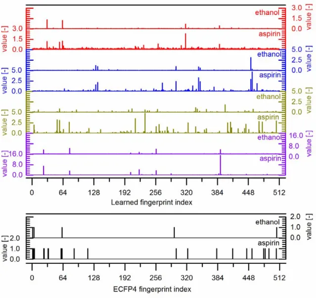
The differences in which features are important in the overall prediction of each property also manifests itself in the fingerprint itself. Figure 13 shows the learned fingerprints for ethanol (SMILES representation, “CCO”) and aspirin (SMILES representation, “O=C(Oc1ccccc1C(=O)O)C”) for four representative models trained on the Abraham, Delaney, Bradley, and multitarget Tox21 datasets; the ECFP4 fingerprint as calculated by RDKit is also provided for reference. The value of the fingerprint at each of the 512 indices is represented by the value of the corresponding bar. Comparing the two compounds’ representations within the same model, it is clear that certain activated indices overlap, corresponding to the similarities between, e.g., the alcohol environment in ethanol and the carboxylic acid or ester groups in aspirin. As expected, aspirin also contains many additional activations not found in ethanol. Due to the random initialization of weights, there is no special interpretation of which indices are activated in particular. Moreover, because each model learns its fingerprint representation at the same time as it learns to predict the target property, the different prediction tasks show different characteristics. For example, the Tox21 model fingerprint has few activations in aspirin not present in ethanol, perhaps due to the fact that aspirin does not contain any additional toxicophores that are necessary to determine toxicity, while the melting point model fingerprint contains numerous additional activations because the additional atom environments in aspirin are indicative of its higher melting point.
Figure 13. Example learned length-512 fingerprints for ethanol and aspirin using representative models for (red) octanol solubility, (blue) aqueous solubility, (brown) melting point, (purple) a multitask model for toxicity, and (black) the fixed ECFP4 fingerprint as implemented in RDKit..
We implement a simplified, linear model to demonstrate how to identify important atoms and atom environments. The convolutional embedding architecture is unchanged, but the hidden neural network layer in the regression portion of the overall model is removed. Accordingly, the most important fingerprint indices can be straightforwardly found by looking at the weights connecting the learned fingerprint to the output layer, analogous to looking at coefficient values in a linear regression model. Then, because the convolutional strategy ends in a pooling approach where individual atom contributions to the fingerprint are summed, the molecular fingerprint is separable into quasi-fingerprints describing atom environments. Example results of such an analysis are shown for a linear model trained on the Delaney dataset in Figure 14. Without any prior chemical knowledge, the model learns that sp2 carbons in nitrogen-containing heterocycles correspond to poor aqueous solubility, while quaternary carbons in aliphatic hydrocarbon neighborhoods with terminal alcohol groups tend to improve aqueous solubility. But, as indicated by the non-highlighted heterocyclic carbons in Figure 14a, this is not a rigid definition corresponding to an exact substructure match. Rather, it is a flexible criterion based on learned feature representation of a chemical environment.
Figure 14. Interpretation of a model trained on the Delaney dataset using a linear regression after convolutional embedding. Highlighted atoms contribute to the two fingerprint indices which most strongly signify (a) low and (b) high aqueous solubility.
Domain of applicability
With any QSAR/QSPR model, it is important to assess the domain of applicability since, fundamentally, any of these models could be applied to any molecule. A straightforward way of estimating prediction error on a novel
compound is to determine the similarity of the target molecule to the molecules used for training. There are many
measures of molecular similarity, but here the Sorensen-Dice coefficient calculated using Morgan circular fingerprints of radius 3 is used as implemented in RDKit. It is worth noting that the learned embeddings here could also serve as the basis of a molecular similarity comparison, although it would be inappropriate to apply that measure to analyze the results of the same model from which it was derived.
Using individual runs of the three representative models, CNN-Ab-oct-representative, CNN-De-aq-representative, and CNN-Br-tm-representative, we assess the prediction uncertainty by examining the absolute error of a target as a function of its “distance” to the training set. The average of the top 5 similarity coefficients appearing in the full dataset is used as a crude measure of this distance. The more unusual molecules, with low average top-5 similarity scores, are expected to have larger prediction errors. These absolute errors are binned, averaged, and displayed in Figure 15 using the sample standard deviation for error bars. The expected trend becomes more apparent and more statistically significant moving from the smallest dataset (Abraham) to the largest (Bradley).
To recapitulate the observed trend, these models – as is expected for all predictive models – are most useful in predicting compounds similar to the compounds on which they were trained. The reported performance values would not hold when applying these models to highly-novel chemicals, particularly those with novel scaffolds. Molecular similarity, as was calculated for Figure 15, provides an estimate of the extent to which a model must extrapolate out of its training domain.
Figure 15. Averaged absolute prediction error for representative models (a) CNN-Ab-oct-representative, (b) CNN-De-aq-representative, and (c) CNN-Br-tm-representative as a function of the averaged top 5 similarity scores among other molecules in each dataset, binned in intervals of 0.1. The Delaney dataset has a single molecule in the 0.1-0.2 interval, so a sample standard deviation cannot be calculated.
Opportunity for attribute improvement
We have incorporated atom-level attributes, both structural and calculable, which are easily found from a 2D representation of a molecule. However, the same framework can incorporate any number of additional atom-level
attributes to differentiate atoms in multiple rings, atomic electronegativity, estimated pKa for hydrogen-containing atoms, hydrogen bonding donor tendency, and hydrogen bonding acceptor tendency. Capturing potential intramolecular
hydrogen bonding and the differences in ring strain enthalpy and entropy should be particularly beneficial to prediction of melting point.
Hyperparameter selection
Model performance is sensitive to the learning rate and schedule, especially in the case of the small Abraham dataset, where the amount of data available for internal validation is quite small. Models were found to be significantly less sensitive to other hyperparameters, i.e. fingerprint length, fingerprint depth, and number of hidden layer nodes, but proper selection of learning rates remains challenging for small datasets (Section S5). Robust optimization of
hyperparameters is computationally expensive, as the many hyperparameter settings and replicates for each
cross-validation fold takes tens of hours to train using one GeForce GTX TITAN graphics card; for this reason, we use a coarse grid search to identify suitable hyperparmeter settings within each fold. Other hyperparameter optimization techniques are certainly compatible with these models and can be accelerated with parallel utilization of multiple graphics cards.50-52
Relationship to descriptor-based models
The key advantage of the convolutional neural network approach to molecular embedding its ability to learn complex relationships between a structure and a prediction target; Duvenaud et al.19 and Kearnes et al.20 have shown that basic structural information is sufficient to make quality predictions. In this work, we have shown significant
improvements in model performance when combining this flexibility with rapidly-calculable atom-level descriptors, which preserves some spatial information related to molecular conformation.
Our combined featurization/convolution strategy avoids the need for exhaustive descriptor calculators like those of CDK or Dragon and avoids the rigidity of the extended connectivity fingerprints. Unlike Abraham linear free energy relationships or Admire’s octanol solubility model, absolutely no empirical solute descriptors or experimental
measurements are required to make a prediction. Although there have been efforts to predict Abraham solute parameters directly from structure53, 54, it is preferable to predict solubility directly when experimental data is available, rather than introducing a 5-parameter bottleneck. The benefit of solvent parameterization (i.e., in using the same solute parameters to predict solubility in different solvents) can be isolated from solute parameterization by incorporating solvent parameters as inputs to a multi-solvent solubility model.
Moreover, the convolutional embedding approach leaves much more room for improvement for future modelling efforts. Descriptor-based molecular representations rely on all relevant information about a molecule being captured in that set of descriptors; no matter how flexible the back-end ( ) is made, the model cannot make use of information that is not provided. By working directly on the full molecular graph, there is a greater opportunity for models to learn how to extract the aspects of a molecule relevant to a prediction task. By expanding the set of atom- and bond-level features and the increasing number of hidden network layers (both within and after the convolutional embedding layer),
similar models would be able to learn implicit attributes which are less directly related to molecular structure and local atom environments.
Relationship to other graph-based approaches
Previous cheminformatics studies have used similar graph-like objects to represent molecules, but pre-processing steps are required to simplify the graph structure. One early technique converts graphs into a lists of discrete substructures of atom pairs separated by a particular graph distance, which can then be mapped to fingerprint-like representations.55 Feature trees can be used for information storage/retrieval and for calculating molecular similarity; however, molecular graphs are necessarily reduced to acyclic trees by combining multiple atoms (particularly those constituting ring structures) into aggregated node.56, 57 Lusci and Baldi describe a similar limitation in their graph-based approach, where cyclic structures must be converted to acyclic graphs.18 Kernel methods (e.g., SVM) can preserve original graph structures by calculating molecular similarity directly using kernels that directly operate on graphs 58-60 The key limitation of this approach is that kernel functions map two graphs to a scalar similarity score and cannot map a single graph to a vector-based representation. This limitation can be mitigated by representing a molecule as a vector of similarity scores
corresponding to that molecule’s similarity to several graph prototypes.61, 62. The approach of preserving the full molecular graph structure and parameterizing the process of its reduction to a vector representation has only recently been
introduced by Duvenaud et al. and Kearnes et al.19, 63.
Limitations of graph-based approach
There are some inherent limitations of a graph-based approach to molecular representation, as also discussed by Kearnes et al.20 Most importantly, precise information related to 3D structure is not easily accessible, although the inclusion of derived atom-level attributes (e.g. Labute approximate surface area contribution) can help mitigate this. The fact that computer programs can calculate approximate 3D structures from simple connectivity information means that a neural network could learn to do the same with sufficient parameterization, although it might not be practically feasible to train such a model with sufficient regularization to avoid overfitting. The lack of 3D positional information also means that stereochemistry is currently ignored. Similarly, a graph representation contains some information about 2D proximity in terms of graph distance, but not a true distance in terms of, e.g., angstroms. Melting points are strongly affected by the solid-phase packing structure (of which multiple polymorphs may exist for a given compound), which in turn relies on intermolecular interactions between substructures that are not necessarily close to each other within a single molecule; the locality of our convolutional approach cannot easily capture this. However, specifying a single conformer to generate 3D descriptors, rather than starting from a 2D representation, would hinder model performance when the chosen conformer is not the conformer most relevant to the prediction task.64
Using octanol solubility, aqueous solubility, melting point, and toxicity assays as example prediction targets, we have demonstrated the use of neural network based models which do not rely on exhaustive molecular descriptor
calculations or experimental parameters. Contrary to what one might expect, learning from basic attributes does not necessitate a large dataset; in the case of octanol solubility, appropriate molecular representations and their relationship to solubility are found with fewer than 200 training examples. These results could encourage a shift away from rigid
molecule-level descriptor calculations and a new paradigm in molecular representation whereby the importance of substructural features and atom environments are learned from atom-level features directly. As the adoption of
convolutional QSAR models continues to grow, development of rapidly calculable atom-level descriptors will become increasingly important.
Extensions of this work include inclusion of other calculable atom-level features, expanding prediction targets to other chemical or physical properties, expanding demonstrations to take advantage of larger datasets, more thorough studies on the use of consensus models and other techniques traditionally used to boost QSAR model performance, and the further exploration of multi-task models.
Corresponding Author
Klavs F. Jensen. Department of Chemical Engineering, Massachusetts Institute of Technology; 77 Massachusetts Avenue, 66-542, Cambridge, MA 02139 (USA); email: [email protected]; homepage: http://web.mit.edu/jensenlab.
Funding Sources
This work was supported by the DARPA Make-It program under contract ARO W911NF-16-2-0023. CWC received additional funding from the NSF Graduate Research Fellowship Program under Grant No. 1122374.
Supporting Information (SI)
Algorithm details, model hyperparameters, and performance metrics for individual runs are tabulated and can be found in the SI. This information is available free of charge via the Internet at http://pubs.acs.org. Full datasets and code are available at https://github.com/connorcoley/conv_qsar_fast.
Abbreviations
MSE, mean squared error; MAE, mean absolute error; SD, standard deviation (of residuals); GSE, general solubility equation; AUROC or AUC, area under the receiver-operator curve.
References
1. Cherkasov, A.; Muratov, E. N.; Fourches, D.; Varnek, A.; Baskin, I. I.; Cronin, M.; Dearden, J.; Gramatica, P.; Martin, Y. C.; Todeschini, R., Qsar Modeling: Where Have You Been? Where Are You Going To? J. Med. Chem. 2014, 57, 4977-5010.
2. Gawehn, E.; Hiss, J. A.; Schneider, G., Deep Learning in Drug Discovery. Mol. Inform. 2016, 35, 3-14. 3. Rogers, D.; Hahn, M., Extended-Connectivity Fingerprints. J. Chem. Inf. Model. 2010, 50, 742-754.
4. Taft, R. W.; Abboud, J.-L. M.; Kamlet, M. J.; Abraham, M. H., Linear Solvation Energy Relations. J. Solution
Chem. 1985, 14, 153-186.
5. Mauri, A.; Consonni, V.; Pavan, M.; Todeschini, R., Dragon Software: An Easy Approach to Molecular Descriptor Calculations. Match 2006, 56, 237-248.
6. Steinbeck, C.; Han, Y.; Kuhn, S.; Horlacher, O.; Luttmann, E.; Willighagen, E., The Chemistry Development Kit (Cdk): An Open-Source Java Library for Chemo-and Bioinformatics. J. Chem. Inf. Comput. Sci. 2003, 43, 493-500. 7. Toropov, A. A.; Toropova, A. P.; Benfenati, E., Qspr Modeling of Octanol Water Partition Coefficient of Platinum Complexes by Inchi-Based Optimal Descriptors. J. Math. Chem. 2009, 46, 1060-1073.
8. Toropov, A. A.; Toropova, A. P.; Benfenati, E.; Gini, G.; Leszczynska, D.; Leszczynski, J., Coral: Qspr Model of Water Solubility Based on Local and Global Smiles Attributes. Chemosphere 2013, 90, 877-880.
9. Cao, D.-S.; Zhao, J.-C.; Yang, Y.-N.; Zhao, C.-X.; Yan, J.; Liu, S.; Hu, Q.-N.; Xu, Q.-S.; Liang, Y.-Z., In Silico Toxicity Prediction by Support Vector Machine and Smiles Representation-Based String Kernel. SAR QSAR Environ. Res. 2012, 23, 141-153.
10. Karwath, A.; De Raedt, L., Smirep: Predicting Chemical Activity from Smiles. J. Chem. Inf. Model. 2006, 46, 2432-2444.
11. Delaney, J. S., Esol: Estimating Aqueous Solubility Directly from Molecular Structure. J. Chem. Inf. Comput.
Sci. 2004, 44, 1000-1005.
12. Eklund, M.; Norinder, U.; Boyer, S.; Carlsson, L., Choosing Feature Selection and Learning Algorithms in Qsar.
J. Chem. Inf. Model. 2014, 54, 837-843.
13. Mitchell, J. B. O., Machine Learning Methods in Chemoinformatics. Wiley Interdiscip. Rev. Comput. Mol. Sci. 2014, 4, 468-481.
14. Dudek, A. Z.; Arodz, T.; Galvez, J., Computational Methods in Developing Quantitative Structure-Activity Relationships (Qsar): A Review. Comb. Chem. High Throughput Screen. 2006, 9, 213-228.
15. Tao, L.; Zhang, P.; Qin, C.; Chen, S.; Zhang, C.; Chen, Z.; Zhu, F.; Yang, S.; Wei, Y.; Chen, Y., Recent
Progresses in the Exploration of Machine Learning Methods as in-Silico Adme Prediction Tools. Adv. Drug Deliver. Rev. 2015, 86, 83-100.
16. Ma, J.; Sheridan, R. P.; Liaw, A.; Dahl, G. E.; Svetnik, V., Deep Neural Nets as a Method for Quantitative Structure–Activity Relationships. J. Chem. Inf. Model. 2015, 55, 263-274.
17. Unterthiner, T.; Mayr, A.; Klambauer, G.; Steijaert, M.; Wegner, J. K.; Ceulemans, H.; Hochreiter, S., Deep Learning as an Opportunity in Virtual Screening. NIPS 2014, 27.
18. Lusci, A.; Pollastri, G.; Baldi, P., Deep Architectures and Deep Learning in Chemoinformatics: The Prediction of Aqueous Solubility for Drug-Like Molecules. J. Chem. Inf. Model. 2013, 53, 1563-1575.
19. Duvenaud, D. K.; Maclaurin, D.; Aguilera-Iparraguirre, J.; Gomez-Bombarell, R.; Hirzel, T.; Aspuru-Guzik, A.; Adams, R. P., In NIPS; 2015, pp 2215-2223.
20. Kearnes, S.; McCloskey, K.; Berndl, M.; Pande, V.; Riley, P., Molecular Graph Convolutions: Moving Beyond Fingerprints. arXiv preprint arXiv:1603.00856 2016.
21. Schütt, K. T.; Arbabzadah, F.; Chmiela, S.; Müller, K. R.; Tkatchenko, A., Quantum-Chemical Insights from Deep Tensor Neural Networks. Nat. Comm. 2017, 8, 13890.
22. Altae-Tran, H.; Ramsundar, B.; Pappu, A. S.; Pande, V., Low Data Drug Discovery with One-Shot Learning. ACS
Cent. Sci. 2017, 3, 283-293.
23. Gómez-Bombarelli, R.; Duvenaud, D.; Hernández-Lobato, J. M.; Aguilera-Iparraguirre, J.; Hirzel, T. D.; Adams, R. P.; Aspuru-Guzik, A., Automatic Chemical Design Using a Data-Driven Continuous Representation of Molecules.
arXiv preprint arXiv:1610.02415 2016.
24. Ragoza, M.; Hochuli, J.; Idrobo, E.; Sunseri, J.; Koes, D. R., Protein–Ligand Scoring with Convolutional Neural Networks. J. Chem. Inf. Model. 2017, 57, 942-957.
25. Segler, M. H.; Kogej, T.; Tyrchan, C.; Waller, M. P., Generating Focussed Molecule Libraries for Drug Discovery with Recurrent Neural Networks. arXiv preprint arXiv:1701.01329 2017.
26. Landrum, G. Rdkit: Open-Source Cheminformatics.
27. Weininger, D., Smiles, a Chemical Language and Information System. 1. Introduction to Methodology and Encoding Rules. J. Chem. Inf. Comput. Sci. 1988, 28, 31-36.
28. Chollet, F. Keras, GitHub: https://github.com/fchollet/keras, 2015.
29. Bastien, F.; Lamblin, P.; Pascanu, R.; Bergstra, J.; Goodfellow, I.; Bergeron, A.; Bouchard, N.; Warde-Farley, D.; Bengio, Y., Theano: New Features and Speed Improvements. arXiv preprint arXiv:1211.5590 2012.