HAL Id: hal-00317784
https://hal.archives-ouvertes.fr/hal-00317784
Submitted on 22 Dec 2004
HAL is a multi-disciplinary open access
archive for the deposit and dissemination of
sci-entific research documents, whether they are
pub-lished or not. The documents may come from
teaching and research institutions in France or
abroad, or from public or private research centers.
L’archive ouverte pluridisciplinaire HAL, est
destinée au dépôt et à la diffusion de documents
scientifiques de niveau recherche, publiés ou non,
émanant des établissements d’enseignement et de
recherche français ou étrangers, des laboratoires
publics ou privés.
dawnside ionosphere induced by successive
exo-magnetosphere pressure pulses
D. V. Sarafopoulos
To cite this version:
D. V. Sarafopoulos. Repetitive X-line Hall current structures over the dawnside ionosphere induced
by successive exo-magnetosphere pressure pulses. Annales Geophysicae, European Geosciences Union,
2004, 22 (12), pp.4153-4163. �hal-00317784�
© European Geosciences Union 2004
Geophysicae
Repetitive X-line Hall current structures over the dawnside
ionosphere induced by successive exo-magnetosphere pressure
pulses
D. V. Sarafopoulos
Department of Electrical and Computer Engineering, Demokritos University of Thrace, Xanthi, Greece
Received: 1 May 2004 – Revised: 20 August 2004 – Accepted: 25 August 2004 – Published: 22 December 2004
Abstract. This work is a synthesis of observational and
mag-netosphere model produced results. In the first place, we ob-serve geographic latitude-dependent delays in signature ar-rival times at dawnside ground magnetograms. We use the IMAGE chain ground station magnetograms associated with in-situ observations obtained from the Wind, ACE, IMP-8, LANL 97A and Cluster satellites. We demonstrate that the structures under study of ground signatures are directly dic-tated by successive exo-magnetosphere pressure pulses ap-plied along the magnetopause. In one case, using the Clus-ter configuration, we deClus-termine the magnetopause surface wave velocity ∼210 km·s−1, the wavelength λ≈16 R
E and
the azimuthal wave number m∼=6. For this case, via Tsyga-nenko’s T96 model, the positions from the ground stations are traced out along the magnetic field lines, and their con-jugate points over the XYGSMplane are determined. In this
way, we have found that especially the conjugate points cor-responding to the highest latitude stations are systematically dispersed along the X-axis (ranging up to ∼8 RE)and
con-sequently, each of these points is associated with a different amount of magnetopause displacement dictated by the pres-sure wave. The local magnetopause compressions produce increments of the cross tail electric field, which is directly mapped over the ionosphere plane, where successive X-line Hall current structures are developed.
Key words. Ionosphere (electric fields and currents) –
Magnetospheric physics (Magnetosphere-ionosphere inter-actions, Electric fields)
1 Introduction
This work is focused on an observational phenomenon with dispersive and latitude-dependent ionosphere structure, which is directly driven by a solar wind pressure pulse. The solar wind/magnetopause/magnetosphere/ionosphere in-teraction is our frame of work, where field line resonances
Correspondence to: D. V. Sarafopoulos
(sarafo@ee.duth.gr)
(FLRs), twin-vortex current systems, pressure induced elec-tric fields, and other involved mechanisms are of great im-portance.
The title of the work summarizes our prime conclusion. Ground and satellite observations are combined with results produced using Tsyganenko’s T96 model. In the observa-tional Sect. 3 representative events are included showing that there is a latitude dependent time delay in the arrival time of ground magnetogram signatures due to exo-magnetosphere successive pressure pulses. Through the T96 model the ground stations are traced out along the magnetic field lines toward the magnetosphere current sheet at ZGSM=0. The
IM-AGE stations mapped close to the dawnside magnetopause are dispersed along the X-axis and, in this way, each station magnetogram carries information which is associated with a different amount of magnetopause displacement, that is it may be possible that information originated from an ex-tent λ/2 of the wavy modulated magnetopause surface corre-sponds to ground stations having the same longitude. There-fore, repetitive solar wind pressure pulses producing tailward travelling waves over the magnetopause may eventually in-duce, as we discuss later on, X-line Hall current structures over the ionosphere.
The fact that a distinct ground signature, at times, dis-plays a latitude-dependent dispersion is not something en-tirely new. We make the following two notes: Sastri et al. (2001) have studied the characteristics of the geomagnetic sudden commencement (SC) that occurred at 12:11:30 UT on 18 November 1993. They observed that the IMAGE stations in the afternoon sector show a latitudinal variation of nomi-nal peak amplitude and peak time across the chain. A similar observation has been found by Takeuchi et al. (2000) for the preliminary impulse (PI) of the negative sudden impulse that occurred at 11:54 UT on 13 May 1995. In both cases, as we checked each event using the T96 model, the IMAGE sta-tions are mapped to azimuthal angles ranging from −45 to
−55◦, over the equatorial plane.
Our inference here, although we have not performed a sta-tistical work, is that events showing the above described dis-persive character are not uncommon and, most importantly,
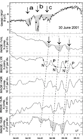
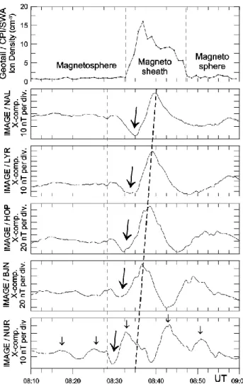
Fig. 1. Three major depressions (labelled (a), (b), and (c)) seen
along the solar wind magnetic field magnitude trace are associated with distinct ground signatures indicating latitude-dependent delays in arrival time. The shaded areas and the thick-dashed lines facili-tate the recognition of the dispersive character.
they are associated with isolated or successive solar wind pressure variations. Additionally, we attempt to define the mechanism producing the dispersive character, and this ef-fort is largely supported by the T96 magnetosphere model. We have selected events observed at the dawnside magne-tosphere because in this sector the T96 model may be able to give the tail-like character of the magnetosphere which is probably more intense closer to the magnetopause.
In a recent work, Sarafopoulos (2004) reported distinct monopolar and bipolar ground signatures, or better, single-and twin-vortex ionosphere current systems, associated with distinct solar wind ram pressure stepwise variations and pulses, respectively. However, he has not studied the dis-persive character observed in signature arrival times, while the latter is the subject we are focused on in this work. Dis-tinct monopolar and bipolar ground signatures are studied by many researchers (Friis-Christensen et al., 1988; McHenry et
al., 1990; Glassmeier and Heppner, 1992; Glassmeier, 1992) but, essentially, they have not associated their events with the interplanetary exo-magnetosphere conditions, or they have not had the presently abundant multi-satellite data. Takeuchi et al. (2002a) studied 28 sudden impulses (SI) events and related solar wind structures to ionospheric twin-vortices. However, they did not consider latitudinal time delays in the ground responses explicitly, and did not apply any magneto-spheric mapping.
It is well-known that the Earth’s magnetosphere cavity is formed by tangential stresses that the solar wind applies, as it gives up momentum to the outer regions of the intrinsic field. In the momentum exchange a system of electric currents is set up whose ¯J × ¯B force effectively distorts the outer fringe of the magnetic field, pulling it downstream to form a comet-like magnetotail. Field lines emerging from the polar regions are swept back, away from the Sun, while field lines originat-ing at low latitudes still form closed loops between Northern and Southern Hemispheres, though there can be some dis-tortion from the dipole form. In this context, we require a quantitative model for the Earth’s magnetic field, in order to calculate geomagnetically conjugate points for the IMAGE array stations over the equatorial plane. We know the geo-graphic coordinates for each ground station, that is the foot-point of a field line at the Earth’s surface, and trace that line for a specified moment of universal time (UT) using Tsyga-nenko’s T96 01 model (the 22 April 2003 version is used). We apply this model in the dawnside magnetosphere and the conjugate points of IMAGE stations are traced over the magnetotail current sheet. These (X, Y)GSMpoints are
deter-mined as those along the field line with ZGSM=0. We use the
new T96 model (Tsyganenko, 1995, 1996), which was devel-oped with continuous dependence on the solar wind pressure, interplanetary magnetic field (IMF) and Dst-index, replacing
earlier binning into several Kp-index intervals.
The observations are exhibited in Sect. 2. The proposed mechanism producing the key observations, together with the results produced through the T96 model, are discussed in Sect. 3.
2 Observations
2.1 First (dawnside) event on 30 June (day 181) 2001 2.1.1 Systematic variation in arrival time of ground
signa-tures
This event clearly shows that distinct ground signatures are systematically detected with progressively increasing time delays at higher latitudes. In Fig. 1, the X-component mag-netograms from five stations (second to sixth panels) with de-creasing latitudes are shown. The geographic, as well as the corrected geomagnetic (CGM), latitudes and longitudes of stations, are shown in Table 1. In the first place, we pay atten-tion to the three major decreases seen by all the Ny ˚Alesund (NAL), Longyearbyen (LYR), Hornsund (HOR), Bear Island
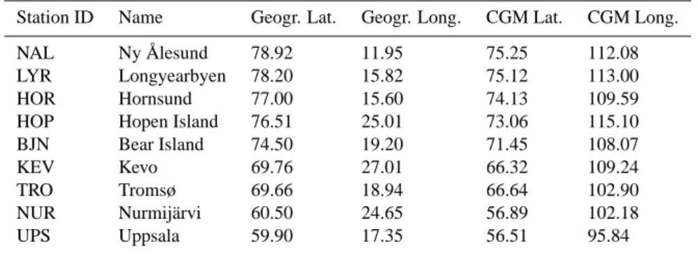
Table 1. Geographical and CGM coordinates of used IMAGE stations.
Station ID Name Geogr. Lat. Geogr. Long. CGM Lat. CGM Long. NAL Ny ˚Alesund 78.92 11.95 75.25 112.08 LYR Longyearbyen 78.20 15.82 75.12 113.00 HOR Hornsund 77.00 15.60 74.13 109.59 HOP Hopen Island 76.51 25.01 73.06 115.10 BJN Bear Island 74.50 19.20 71.45 108.07
KEV Kevo 69.76 27.01 66.32 109.24
TRO Tromsø 69.66 18.94 66.64 102.90
NUR Nurmij¨arvi 60.50 24.65 56.89 102.18 UPS Uppsala 59.90 17.35 56.51 95.84
(BJN), and Nurmij¨arvi (NUR) stations; these decreases are shaded in the second and bottom panels. Their minimum values show systematic delays in arrival time, a fact that is underlined through the thick-dashed lines. The three major decreases are seen at stations with latitudes from 56.8◦(NUR station) to 76.07◦(NAL station), that is in a range of ∼20◦, which probably suggests that the whole magnetosphere is af-fected in a global scale mode. Certainly some field line res-onances (FLRs) are inevitably observable along a few sta-tion (for instance, BJN or NUR) traces, but the FLR pul-sations are superimposed over the dominant and permanent three-peaked structure. The higher latitude stations display the larger magnitude decreases; a piece of providing strong evidence that the disturbances under study are damping at larger distances from the magnetopause. Additionally, the maximum observed delay time of ∼6 min is shared among the five-latitude station steps included in Fig. 1. The dia-gram for each ground signature arrival time versus the ge-ographic latitude of station is shown in Fig. 2. The solid circles correspond to the stations of Fig. 1 and the dashed line Y=2.85lnX+73.65 represents a fitting curve. In Fig. 2 the open circles show the computed ground signature veloc-ity that is almost constant for the stations poleward of BJN and ∼1.7 km s−1. The ultimate mechanism producing the de-lays must quantitatively produce the velocity-station latitude scheme of Fig. 2. Our next step is to provide convincing ob-servational evidence that the three presented decreases along the magnetogram traces are caused by three successive and distinct exo-magnetospheric pressure increases, the so-called pressure pulses.
2.1.2 Three successive solar wind pressure pulses
In the upper panel of Fig. 1 the intrinsic (i.e. unaffected by the bow shock) interplanetary magnetic field (IMF) magnitude is shown, demonstrating three major depressions labelled as a), b), and c). We shall argue below that these depressions are as-sociated with three solar wind pressure pulses, which are the direct drivers for the ground signatures under study. The IMF magnitude of Fig. 1 is measured by Geotail located at (X, Y, Z)GSE=(15.27, 2.43, 1.66) RE, at 05:00 UT. The Geotail, as
well as the ACE, LANL 97A and Cluster 3 positions, and the
Fig. 2. For the five X-component ground magnetograms of Fig. 1
the arrival times for each signature are shown versus the station lat-itudes (solid circles). The arrival time at NUR station is considered as reference. The nonlinear character of the fitting line shown is apparent: the time delay for the highest latitude stations is very sen-sitive to latitude variations. The computed ground signature veloci-ties are shown with open circles.
average IMF direction, are shown in Fig. 3. The geographic longitude for the Geostationary satellite LANL 97A is 70.2◦, and at 05:00 UT its position is shown in Fig. 3. ACE, at the same time, was positioned at (X, Y, Z)GSE=(247.8, 20.4,
14.3) RE.
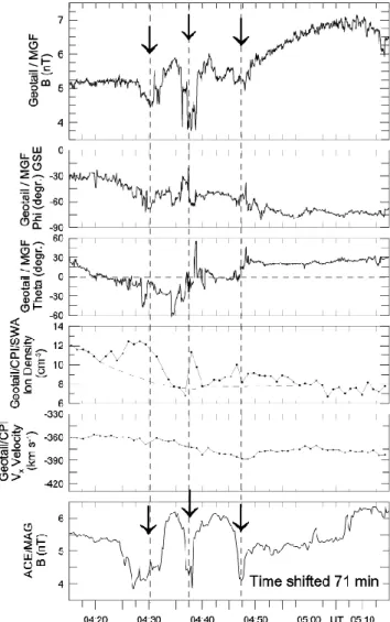
The Geotail/MGF experiment vector magnetic field mea-surements (magnitude B, azimuthal phi and polar theta an-gles), for the interval under study, are shown in Fig. 4 (top three panels). The three magnitude decreases are associated with three magnetic field decreases observed 71 min before by the ACE spacecraft (Fig. 4, bottom panel). This value of travel time is close to the expected, if we take into account the solar wind velocity being Vx=360 km/s (fifth panel), and the separation distance between Geotail and ACE 1X=232 RE.
Fig. 3. Geotail, ACE, LANL 97A and Cluster 3 satellite positions
(solid circles) projected over the XYGSE plane are shown for the
event of day 181, 2001, at 05:00 UT. The IMF direction and the propagating pressure pulse front in the solar wind are also drawn (dashed lines). The points NUR, BJN, HOP, LYR and NAL (open circles) are the conjugate points (determined via the T96 model) for these stations over the XY plane.
These three successive magnetic field magnitude varia-tions correspond to three dynamic pressure increases, as it is inferred by the following in-situ measurements:
– There are three solar wind density enhancements seen
along the Geotail/CPI/SWA trace (Fig. 4, fourth panel) that are anticorrelated to the magnetic field decreases. Additionally, at the same time, the solar wind velocity Vx(fifth panel) essentially remains unchanged. – The three solar wind magnetic field decreases seem to
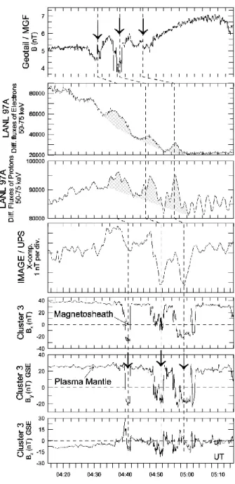
be closely anti-correlated to variations of energetic par-ticle fluxes at the LANL 97A site. Actually, Fig. 5 shows “the three exo-magnetosphere pulses” to be tightly associated with increases seen along the ener-getic electron and proton (50–75 keV) differential fluxes (second and third panel, shaded areas).
– The earliest detected response at ground is that
cor-responding to the lowest latitude stations of the IM-AGE array, and representatively the Uppsala (UPS) X-component response is shown in the fourth panel of Fig. 5. The vertical dashed lines show the systematic time delays at different sites, demonstrating that the successive compression fronts are essentially aligned to the direction of the average IMF, as it is drawn in
Fig. 4. Geotail/MGF vector magnetic field measurements along
with the Geotail/CPI/SWA ion density and velocity. At the bot-tom panel, the ACE/MAG trace of the solar wind magnetic field magnitude is time-shifted 71 min to match the Geotail data.
Fig. 3. The dayside magnetosphere is compressed first, and later the dawnside section where the IMAGE sta-tions are mapped. The NUR, as well as the NAL, LYR, Hopen Island (HOR) and BJN open circle points marked in Fig. 3 are the conjugate points for these sta-tions over the equatorial plane computed via Tsyga-nenko’s T96 model. The compression travel time from Geotail to LANL 97A (8 min, on average) is, as antic-ipated, larger than that between LANL 97A and UPS (5 min on average). Certainly we assume that the inci-dent pressure force is peaked when it is applied perpen-dicularly to the magnetopause surface.
– The Cluster four satellites provide additional evidence
supporting the existence of three pressure increases travelling along the magnetopause surface (Fig. 5, three bottom panels), as we shall study in detail in Sect. 2.1.3. Therefore, with in-situ measurements upstream of the bow
Fig. 5. From top to bottom, Geotail/MGF solar wind magnetic field
magnitude, LANL 97A differential fluxes of energetic (50–75 keV) electrons and ions inside the magnetosphere, IMAGE UPS sta-tion X-component magnetogram on the Earth’s surface, and Clus-ter 3 magnetic field measurements (Bx,By and Bzcomponents) at
the plasma mantle/magnetosheath region, are shown. The magne-tosheath proper is characterized by negative By values, while the
vertical dashed lines mark the different arrival times of signals pro-duced by solar wind pressure variations at different places.
shock, as well as inside the magnetosphere cavity, convinc-ing evidence for three successive solar wind pressure pulses is achieved.
2.1.3 Velocity of the magnetopause surface wave
The Cluster 3 spacecraft, at 05:00 UT, was positioned at (X, Y, Z)GSE=(−1.9, −10.67, 8.56) RE, and Cluster 1, 2, and 4,
Fig. 6. Two brief entries of Cluster 1 and 2 into the plasma mantle
proper (shaded regions with positive Byvalues). The two satellites
separated along the X-axis diagnose a shift in arrival time of magne-topause boundary which is due to a surface wave travelling tailward with a velocity 210 km s−1.
relatively to Cluster 3, were positioned at
(1X1, 1Y 1, 1Z1) = (323, −1918, 1907) km,
(1X2, 1Y 2, 1Z3) = (−1550, −2715, 1542) km, and
(1X4, 1Y 4, 1Z4) = (−1688, −4357, 389) km.
Cluster 3 remains at the high-latitude boundary layer (HLBL), called the plasma mantle. When a solar wind pressure pulse reduces the magnetotail diameter, Cluster 3 crosses the boundary and exits into the magnetosheath. The latter is evident from the bottom three panels of Fig. 5, show-ing the Cluster 3 magnetic field (FGM experiment, Balogh et al., 1997) components. The negative values along the By
trace represent the magnetic field lines that are draped around the magnetopause (Ohtani and Kokubum, 1991; Sarafopou-los, 1995). The IMF has an intense negative (about −3 nT, see Fig. 4) By component, which is detected in each
Clus-ter exit into the magnetosheath proper. Therefore, the three successive exits of Cluster 3 are caused by three compres-sions applied over the magnetopause. The resulted sur-face wave propagates tailward and its velocity can be esti-mated using the geometry of four Cluster spacecraft. The most appropriate spacecraft positions are those of Cluster 1 and 2, which are mainly separated along the X-axis (i.e.
1X12=1873, 1Y12=797 and 1Z12=365 km). Figure 6 shows
two representative short-lived entries of both Cluster 1 and 2 into the plasma mantle (positive By values). The travel time
from Cluster 1 to 2 is about 1t=9 s and the derived surface wave velocity along the magnetopause is ∼210 km·s−1. The wavelength for the surface wave is ∼16 RE,given that the
wave period is 8 min. Approximating the Cluster 3 L-shell as circular, we obtain a circumference of ∼95 RE, and the
azimuthal wave number is m∼=6, which is obviously a low wave number (m<10).
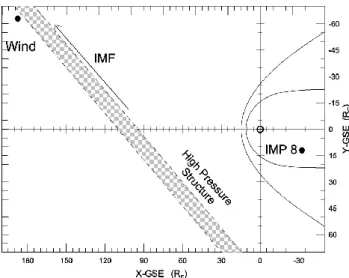
Fig. 7. Wind and IMP-8 positions, projected over the XYGSEplane,
for the event of day 29, 1995. A high pressure structure in the solar wind is indicatively shown, as well as the direction of the IMF.
2.2 Second (dawnside) event on 29 January (day 29) 1995
In this case study the solar wind conditions have been moni-tored by the Wind spacecraft located at (X, Y, Z)GSE=(182.3,
−64.4, −9.4) RE, at 06:00 UT of day 29, 1995 (Fig. 7).
Mea-surements obtained on board Wind are shown in the upper three panels of Fig. 8, and demonstrate the existence of four major solar wind dynamic pressure increases. Four decreases seen along the IMF Bxcomponent trace (top panel) are
an-ticorrelated to the ion (second panel, thick line) and electron (thin line in descending scale) densities, which are obtained by the Wind/3DP and Wind/SWE instruments, respectively. The Wind/SWE ion dynamic pressure (in nPa, third panel) has almost a similar time profile with that of ion density. We note that all the displayed data of Wind are shifted in time 39 min to offset the solar wind convection time from Wind to Earth. The four pressure increases are applied over the magnetosphere and the IMAGE array ground magnetograms are modulated by them. The highest latitude NAL station shows four major peaks (marked with arrows along the X-component trace in Fig. 8), during the period 06:40−07:55 UT of day 29, 1995. These major peaks are also detected at lower latitudes by the Hornsund (HOR), HOP and BJN stations. Most significantly, these peaks are associated with latitude-dependent time delays. In the HOP station trace we discern more than three peaks, and all the peaks are fully de-veloped at the BJN station site. It seems that a FLR is devel-oped at the BJN station magnetic flux tube because the BJN L-shell field line eigenperiod probably matches better with the repetition rate of the excitation source. At lowest lati-tude stations (not shown in Fig. 8), the four solar wind driven peaks are seen as transient magnitude decreases. Addition-ally, these four pressure increases probably dictate the de-viations seen along the By-component of the magnetic field
measured by IMP 8 (bottom panel), which was located at (X,
Fig. 8. From top to bottom, Wind/MFI magnetic field Bx
compo-nent, Wind/3DP ion density (thick line) and Wind/SWE electron density (thin line, in descending scale), Wind/SWE ion pressure in nPa (third panel), NAL, HOR, HOP and BJN station X-component magnetograms, and the Bycomponent of the magnetosphere
mag-netic field as measured by IMP 8 (bottom panel).
Y, Z)GSE=(−31.6, 13, 12.8) RE, within the magnetosphere
cavity.
In summary, it seems that the four distinct pressure varia-tions immediately produce ionospheric currents in the high-est latitude stations that naturally correspond to magnetic flux tubes closest to the magnetopause. The currents are exter-nally driven and display similar time profiles with the solar wind density trace. A second mechanism (i.e. a FLR) pro-duces pulsations with a period T∼=8 min at lower latitude sta-tions and especially at BJN. The high pressure solar wind structures seem to be directly associated with the IMF direc-tion. In Fig. 7 the shaded high-pressure region with a dura-tion of ∼4 min sweeps the Wind, as well as the IMP-8 sites.
2.3 Third event on 15 October (day 288) 2001
A particular characteristic for this event is that it has been caused by an isolated solar wind pressure increase. The later is better manifested through the Geotail/CPI/SWA ion density trace shown in the top panel of Fig. 9. Geotail, at 08:00 UT, was located at (X, Y, Z)GSM=(6.8, 12, −4.6) RE.
At ∼08:33 UT Geotail temporarily exits from the magneto-sphere/boundary layer region into the magnetosheath charac-terized by high density values. We identify the initial Geotail entry into the magnetosphere at ∼08:00 UT by an abrupt in-crease in Bz and earthward fluxes of the ∼60 keV energetic
particles (not shown here). The short exit into the magne-tosheath is not accompanied with energetic particle fluxes measured by Geotail/EPIC. The systematic delays in arrival times of ground signatures are apparent, and the thick-dashed line in Fig. 9 underlines this fact. The small arrows along the NUR station trace suggest that a FLR is developed at this flux tube. This event occurred at the pre-noon rather than the dawnside section of the magnetosphere.
Our assumption that the magnetosphere was compressed and Geotail was forced to exit from the magnetosphere is largely supported by the Wind data (not shown here). Wind was located at (X, Y, Z)GSE=(67.5, −58, 7.8) RE, at
08:00 UT. For a long time the ion density remains fluctuating at a level of ∼4 cm−3(3DP plasma experiment) and abruptly
changes to ∼7 cm−3at ∼07:58 UT. This transition is applied over the magnetosphere after ∼32 min, and this is the antici-pated travel time resulting from the measured solar wind ve-locity ∼430 km s−1and the appropriate interplanetary pres-sure discontinuity orientation. The latter is evaluated from the time-lag responses between Wind and Geotail/ground stations: the pressure front must be inclined so that the dis-continuity normal has a longitude of ϕ∼135◦. Certainly this orientation will be slightly modified after crossing the bow shock because of refraction (Sarafopoulos, 2004). Eventu-ally, the pressure front inclination suffices to excite a local magnetopause surface waveform travelling tailward and pro-ducing the ground dispersive signatures.
3 Discussion
3.1 Systematic latitude-dependent delays related to results from the T96 model
Our main inference in this work is that a solar wind pres-sure pulse produces a ground signature that is detected with a time delay positively correlated to the station latitude: the higher the latitude, the larger the delay time. Therefore, we would anticipate that successive, quasi-periodic pressure pulses might produce latitude-depended ground waveforms, even in anti-phase. Actually, this is the case for the event shown in Fig. 1: the NAL and BJN stations detect waves in anti-phase. An explanation for this observational feature, in terms of ionospheric currents, is given later on, together with an appropriate schematic figure.
Fig. 9. Geotail for a short time period (∼12 min) exits from the
magnetosphere into magnetosheath and the CPI/SWA ion density increases. This exit is imposed by a solar wind pressure increase (not shown here), while the selected X-component magnetograms from the IMAGE stations show dispersive character in signature ar-rival times.
At present, we are interested in determining the conjugate points for the IMAGE stations over the magnetosphere equa-torial plane. It is reasonable for one to anticipate that the higher latitude stations will map at points displaced progres-sively tailward, given that the magnetic field shells near the magnetopause are pulled tailward by the solar wind. In our first two case studies the IMAGE stations are close to the dawn meridian plane and, therefore, they will probably carry information associated with the dawnside magnetopause sur-face waves.
We use the T96 model in order to calculate the geomag-netically conjugate points for the IMAGE array stations over the magnetotail current sheet plane. For our first case (30 June 2001), we define the universal time (04:50 UT), the ge-ographical longitude and latitude for each station, the solar wind dynamic pressure 2 nPa, and the Dst=18 nT. The Byand
Bz components of the IMF (from the Geotail data, Fig. 4)
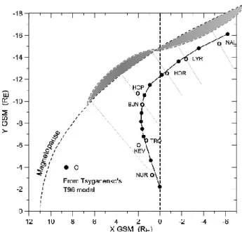
Fig. 10. The open circle points are determined via the T96 model
as the conjugate point of these ground stations over the XYGSM plane. The solid circles are produced, again, via the T96 model for a hypothetic ground chain of stations with constant latitude equal to 19.2◦. This figure corresponds to the event of day 181, 2001, at 05:00 UT, with Dst=18 nT, IMF By=−3 nT and Bz=−1 nT, and
solar wind pressure 2 nPa. For this event, the magnetopause sur-face wavelength is ∼16 RE, and therefore different stations are
as-sociated with different amounts of magnetopause surface displace-ments.
Fig. 11. Three hypothetic chains of ground stations with constant
longitudes (i.e. 9.2, 19.2 and 29.2◦) are traced out along the mag-netic field lines via the T96 model and their conjugate points over the XYGSMplane are determined, for the conditions of the event which occurred on day 181, 2001.
eight open circles represent the conjugate points for the sta-tions NUR, Kevo (KEV), Tromsø (TRO), BJN, HOP, HOR, LYR and NAL over the XYGSMplane. Additionally, the solid
circles in the same figure correspond to a hypothetic chain of ground stations having progressively increasing latitudes, while their longitudes are the same. More specifically, all the stations in this hypothetic chain have longitude 19.2◦, which is the longitude of station BJN considered as refer-ence. The three solid circles closer to the Earth correspond to 60.5, 65.5 and 70.5◦geographic latitudes, while the next ten points correspond to latitudes with increment 1◦, that is the more distant point from the Earth has latitude 80.5◦and longitude 19.2◦.
A profound conclusion is that the lower latitude stations (60.5−70.5◦)are mapped at almost radial positions, whereas
the higher latitude (71.5−80.5◦) magnetic field lines are
pulled downstream. This result, the qualitatively anticipated one, is probably the cause for the detected dispersion in ground signature arrival times. A supposed tailward travel-ling compression pulse along the magnetopause will proba-bly produce a poleward travelling signature in ground mag-netograms.
Figure 10 is drawn for the first studied event for which the magnetopause wave velocity is estimated V=210 km s−1 and the surface wavelength ∼16 RE. The latter is
schemat-ically visualized in Fig. 10, where the shaded area shows the compressed-decompressed part of the magnetosphere. It is apparent that each station is associated with a different amount of magnetopause displacement from its nominal po-sition. Most importantly, for instance, the NAL station cor-responds to a highly compressed region, whereas the BJN station corresponds to a highly decompressed region. Ob-servationally, the stations NAL and BJN show waveforms in anti-phase and, therefore, this feature is probably directly as-sociated with the magnetopause surface wave.
We have mentioned in the Introduction 2 cases cited by Takeuchi et al. (2000) and Sastri et al. (2001), showing lati-tude dependence on signature arrival times. Although both of them were observed in the post-noon section, the production mechanism may be similar to what is proposed in this work. 3.2 Longitude-dependent response in the T96 model At this point, we think that it is of great importance to scru-tinize more systematically how the different longitudes of IMAGE stations may affect our mechanism producing dis-persion patterns. It is useful to check the influence of lon-gitude using three hypothetic chains of ground stations with constant geographic longitude in each chain. We consider the three chain-categories having longitudes 9.2◦, 19.2◦and 29.2◦, that is we assume a fluctuation range ±10◦, as it is the situation for the IMAGE stations. Figure 11 shows the results for the three categories (stars, solid and open circles) produced via Tsyganenko’s T96 model. The geographic lat-itudes are shown along the left-hand dashed line of Fig. 11, ranging from 60.5◦to 80◦. All three categories demonstrate the same trend: the higher latitude magnetic field lines are
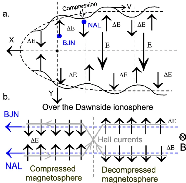
Fig. 12. (a) Sketch showing three successive compressions applied over the magnetopause surface from three successive solar wind pressure
pulses. Each compression is associated with a local increment 1E of the cross-tail electric field, which is travelling tailward. The solid circles BJN and NAL are the conjugate points for these stations over the XY plane. (b) The increments 1E travelling tailward and sweeping the BJN and NAL sites over the XY plane are directly mapped over the ionosphere plane. In this sketch the NAL station with the highest latitude and the station BJN as well are assumed to move sunward beneath the ionosphere structure of 1E considered stationary. The X-line Hall current configuration inferred from ground measurements is drawn with a thick grey line.
mostly displaced tailward. At this point we pay attention to the IMAGE chain longitudes and their influence over the de-rived pattern. We underline the fact that the specific array of the NAL, LYR and HOP stations with increasing longi-tudes (i.e. 11.5◦, 15.82◦and 25.01◦, respectively) reinforces further their dispersion along the X-axis.
3.3 Pressure wave producing X-line Hall current structures over the ionosphere
In schematic Fig. 12a, we consider that the magnetopause un-dulates over the XY plane with a surface velocity V. Each of the successive compressions (decompressions) shown
corre-sponds to an inward (outward) bulge of the magnetopause surface. Moreover, we assume that each local compres-sion diminishes the magnetotail width and consequently, pro-duces an increment 1E of the cross tail electric field E. In the first studied event, the three successive compressions will give a waveform 1E=1E0sin(kx+ωt) travelling tailward
with a velocity ∼210 km·s−1. This is visualized in Fig. 12a
with alternating direction in the 1E vectors. Additionally, the conjugate points for the stations NAL and BJN over the XY plane are indicatively placed in Fig. 12a. It is obvious that NAL is mapped to a region with positive 1E incre-ment, whereas BJN is mapped to a region with negative 1E increment. This placement is realistic given that the
mag-netopause surface wavelength and the distance between the NAL and BJN points are estimated ∼16 and 8 RE,
respec-tively. The 1E variations are carried through the magnetic field lines and directly applied over the ionosphere plane, which is shown in Fig. 12b. In this schematic the ground stations NAL and BJN are considered to be moving sunward below a hypothetic stationary structure of ionospheric 1E electric fields. These electric fields, together with the local magnetic fields, produce Hall currents, which are detected by both ground stations as bipolar magnetic field variations (i.e. NP for BJN, and PN for the NAL station). In Fig. 12b an X-line structure of Hall currents is formed and probably it is part from a twin-vortex current system. According to recent work by Sarafopoulos (2004), each solar wind pres-sure pulse produces a distinct Positive/Negative (PN) or Neg-ative/Positive (NP) bipolar feature along the X-component magnetogram traces, and most importantly, each pulse is associated with a twin-vortex ionospheric current structure. Therefore, under this perspective, in our first case study, the three bipolar NP pairs that are marked along the LYR sta-tion trace in Fig. 1 (third panel), probably provide strong ev-idence for three twin-vortex ionospheric current structures. In this work, we do not have the cases of single pressure pulses analyzed by Sarafopoulos (2004); however, the con-clusion here is that even the more complicated events with repetitive pulses will produce recurrent twin-vortex systems, like the example of multiple vortices shown by McHenry et al. (1990).
3.4 FLRs and observed ground signals
Certainly the observed phenomenon with gradual increases in arrival times of ground signatures is latitude-dependent and produces waveforms out of phase, and even in anti-phase. This observation is entirely different from the field line resonance (FLR) mode of oscillation, although the FLR produces waves that change their polarization (waves in anti-phase) when crossing the resonant L-shell. In our study the amplitudes of a ground signature are maximized at the highest latitude stations mapped closest to the magnetopause boundary. In contrast, in the FLR mode of oscillation a res-onance region of about 1◦latitudinal width, at ground, is ex-cited, and corresponds to a particular L-shell (Walker et al., 1979; Hughes, 1994; Glassmeier, 1995). Most importantly, our ground response seems to be directly associated with the solar wind exo-magnetosphere conditions rather than an intra-magnetosphere dynamics. Certainly the above discus-sion does not refuse the existence of authentic FLR events and the validity of the FLR theory as well.
3.5 The magnetosphere/ionosphere velocity scale factor The detected dispersive structures are mainly produced by the stations having higher latitudes than that of BJN. Usually BJN constitutes the threshold latitude in curves like those of Figs. 2 and 10. The tailward travelling magnetopause sur-face wave produces a northward moving ionosphere signa-ture. The magnetopause surface velocity (see Fig. 10)
pro-duces a magnetosphere pressure wave propagating from the point BJN to point NAL, with an almost constant velocity value of ∼210 km s−1. The ionosphere velocity for a distinct
current signature, at higher latitudes than the BJN one, is al-most constant and ∼1.7 km s−1(see Fig. 2). Therefore, there is a velocity scale factor between the two propagating waves of ∼130. The ground stations from the IMAGE array having latitudes smaller than that of BJN are associated with almost radially placed conjugate points over the equatorial plane. If the line connecting these points is orthogonal to the mag-netopause surface, then the ground stations will respond in-stantly and there is not any delay time. Apparently the curve of Fig. 2 is not fully associated with the curve of Fig. 10; Fig. 2 is lacking the information of station longitude. The above determined scale factor is of great importance because one can reliably estimate the magnetopause surface velocity knowing the ground signature northward velocity, which is always calculable from the available ground data.
3.6 Orientation of the pressure wave front
A fundamental notion in this work is that the studied disper-sive ionosphere structures are directly produced by tailward travelling magnetopause surface waves. In order to be de-tected ground delays, two factors are of critical importance. First, the conjugate points of ground stations over the equa-torial plane must be dispersed along and close to the magne-topause surface and second, the excited magnemagne-topause sur-face wave must have a wavelength comparable to the extent of the dispersed ground station conjugate points over the XY plane. The maximum delay time is dependent on the sur-face wave velocity and the extent of dispersion of ground sta-tion conjugate points along the magnetopause. Apparently, if we hypothesize a pressure wave front parallel to the magne-topause, then no dispersive structures on Earth will be an-ticipated, although a ground response will exist. Therefore, a highly inclined pressure discontinuity orientation may be-come of great importance, as was the case in determining the geomagnetic sudden commencement (SC) rise time by Takeuchi et al. (2002b).
4 Conclusions
Ground and satellite observations, together with results from Tsyganenko’s T96 model of the magnetosphere, have estab-lished the conditions under which a compression wave trav-elling tailward along the magnetopause surface will produce poleward moving signatures in ground magnetograms. We observe geographic latitude-dependent delays in signature arrival times at dawnside ground magnetograms and demon-strate that these structures are directly dictated by successive exo-magnetosphere pressure pulses applied along the mag-netopause. The phenomenon of observed gradual increases in arrival times of ground signatures produces waveforms out of phase, and even in anti-phase. The studied events are as-sociated with twin-vortex ionosphere structures and are
en-tirely different from the field line resonance (FLR) mode of oscillation. In our study the amplitudes of a ground signature are maximized at the highest latitude stations mapped clos-est to the magnetopause boundary. The maximum delay time in ground dispersed structures is dependent on the magne-topause surface wave velocity and the extent of dispersion of ground station conjugate points over the equatorial plane and along the magnetopause. In one case, with in-situ measure-ments, we determine the magnetopause surface wave veloc-ity ∼210 km·s−1, the magnetopause wavelength λ≈16 RE
and the azimuthal wave number m∼=6. For the same case study, the ionosphere signature velocity produced from the magnetopause surface wave, at higher latitudes than the BJN station one, is almost constant and ∼1.7 km s−1. Therefore, there is a velocity scale factor of ∼130 between the waves propagating along the magnetopause surface and those mov-ing northward in ionosphere and producmov-ing the ground dis-persive structures.
Acknowledgements. We are grateful to all Principal Investigators
of the experiments MGF and CPI/SWA of Geotail; MFI, 3DP and SWE of Wind; MAG of ACE and IMP 8; FGM of Cluster and the energetic particle experiment of LANL 97A. Concerning the use of ground magnetometer data, we are grateful to the Finnish Meteo-rological Institute (FMI/GEO), the Technical University of Braun-schweig and other institutes that maintain the IMAGE magnetome-ter array. The author thanks both of referees.
Topical Editor T. Pulkkinen thanks A. Viljanen and another ref-eree for their help in evaluating this paper.
References
Balogh, A., Dunlop, M. W., Cowley, S. W. H., Southwood, D. J., Thomlinson, J. G., and the Cluster magnetometer team: The Cluster Magnetic Field Investigation, Space Sci. Rev., 79, 65– 92, 1997.
Friis-Christensen, E., McHenry, M. A., Clauer, C. R., and Venner-strom, S.: Ionospheric travelling convection vortices observed near the polar cleft: A triggered response to sudden changes in the solar wind, Geophys. Res. Lett., 15, 253–256, 1988. Glassmeier, K.-H.: Travelling magnetospheric convection
twin-vortices: observations and theory, Ann. Geophys., 10, 547–565, 1992.
Glassmeier, K.-H. and C. Heppner: Travelling magnetospheric con-vection twin vortices-Another case study, global characteristics, and a model, J. Geophys. Res., 97, 3977–3992, 1992.
Glassmeier, K. H.: ULF pulsations, in Handbook of Atmospheric Electrodynamics, Volume II, Edited by H. Volland, 463–502, University of Bonn, Germany, 1995.
Hughes, W. J.: Magnetospheric ULF waves: A tutorial with a his-torical perspective, in Solar Wind Sources of Magnetospheric ULF Waves, Geophys. Monogr. Ser., vol. 81, edited by M. J. Engebretson, K. Takahashi, and M. Scholer, 1–11, AGU, Wash-ington D.C., 1994.
McHenry, M. A., Clauer, C. R., and Friis-Christensen, E.: Rela-tionship of solar wind parameters to continuous, dayside, high-latitude travelling ionospheric convection vortices, J. Geophys. Res., 95, 15 007–15 022, 1990.
Ohtani, S. and Kokubum, S.: Magnetic properties of the high-latitude tail boundary: Draping of magnetosheath field lines and tail-aligned current, J. Geophys. Res., 96, 9521–9530, 1991. Sarafopoulos, D. V.,: Long duration Pc5 compressional pulsations
inside the Earth’s magnetotail lobes, Ann. Geophys., 13, 926-937, 1995.
Sarafopoulos, D. V.: Distinct solar wind pressure pulses produc-ing convection twin-vortex systems in the ionosphere, Ann. Geo-phys., 22, 2201–2211, 2004.
Sastri, J. H., Takeuchi, T., Araki, T., Yumoto, K., Tsunomura, S., Tachihara, H., Luehr, H., and Watermann, J.: Preliminary im-pulse of the geomagnetic storm sudden commencement of 18 November 1993, J, Geophys. Res., 106, 3905–3918, 2001. Takeuchi, T., Araki, T., Luehr, H., Rasmussen, O., Watermann, J.,
Milling, D. K., Mann, I. R., Yumoto, K., Shiokawa, K., and Na-gai, T.: Geomagnetic negative sudden impulse due to a magnetic cloud observed on 13 May 1995, J. Geophys. Res., 105, 18 835– 18 846, 2000.
Takeuchi, T., Araki, T., Viljanen, A., and Watermann, J.: Ge-omagnetic negative sudden impulses: Interplanetary causes and polarization distribution, J. Geophys. Res., 107(A7), doi: 10.1029/2001JA900152, 2002a.
Takeuchi, T., Russell, C. T., and Araki, T.: Effect of the orientation of interplanetary shock on the geomagnetic sud-den commencement, J. Geophys. Res., 107(A12), 1423, doi: 10.1029/2002JA009597, 2002b.
Tsyganenko, N. A.: Modelling the Earth’s magnetospheric mag-netic field confined within a realistic magnetopause, J. Geophys. Res., 100, 5599–5612, 1995.
Tsyganenko, N. A.: Effects of the solar wind conditions on the global magnetospheric configuration as deduced from data-based field models, European Space Agency Spec. Publ., ESA SP-389, 181, 1996.
Walker, A. D. M., Greenwald, R. A., Green, C. A., and Stuart, W.: STARE radar auroral observation of Pc5 geomagnetic pulsations, J. Geophys. Res., 84, 3373–3388, 1979.