A dynamic model of locomotion for computer animation

(1)

A DYNAMIC MODEL OF LOCOMOTION FOR

COMPUTER ANIMATION

BY

MICHAEL ALLEN MCKENNA

Bachelor of Science

Massachusetts Institute of Technology Cambridge, MA. 1987

Submitted to the Media Arts and Sciences Section in partial fulfillment of the

requirements for the degree of MASTER OF SCIENCE

at the

Massachusetts Institute of Technology February 1990

Signature of the Author

Certified by _

Accepted by

Michael A. McKenna Media Arts and Sciences Section January 12, 1990

David L. Zeltzer Thesis Supervisor so(i te of nCorputer Graphics

t/

-- 'S-'ephen A. Benton

Chairman, Departmental Committee on Graduate Studies gASsACHusETTs iSTITTE

OF TECHNOLOGY

(2)

Document Services Room 14-0551 77 Massachusetts Avenue Cambridge, MA 02139 Ph: 617.253.2800 Email: docs@mit.edu http://libraries.mit.edu/docs

DISCLAIMER NOTICE

The accompanying media item for this thesis is available in the MIT Libraries or Institute Archives.

(3)

A DYNAMIC MODEL OF LOCOMOTION FOR COMPUTER ANIMATION

BY

MICHAEL ALLEN MCKENNA

Submitted to the Media Arts and Sciences Section on January 12, 1990, in partial fulfillment of the

requirements for the degree of Master of Science

Abstract

A computational model of legged locomotion was developed in which all

mo-tions are physically-based. A dynamic simulator for articulated figures forms the basis of all motion in the system, where forces are applied to bodies, and their

accelerations are then computed. A gait controller coordinates the activity of stepping and stance, and is based on biological mechanisms found in

vertebrates and invertebrates. Dynamic motor programs, based on spring and damper combinations, provide the forces required to move the limbs in order to step and to propel the body forward. The system successfully computes the mo-tions of a simulated six-legged insect negotiating level and uneven terrain.

A VHS videotape containing sample animations accompanies this thesis.

Thesis Supervisor: David L. Zeltzer

Title: Associate Professor of Computer Graphics

This work was supported in part by the National Science Foundation (Grant

IRI-8712772), and equipment grants from Hewlett-Packard Co., Gould Electronics,

(4)

Acknowledgements

I would like to first thank Dave Small, the person I can rely on more than any

other.

And thanks to my Mom, for sending me to MIT, and for so much encouragement.

Thanks to my advisor, David Zeltzer, for introducing me to so many new con-cepts.

And of course, thanks to all the Snakepit guys for stimulating conversation, and much needed diversion.

(5)

In recent years, the field of computer animation has been turning more and more to dynamic simulation in order to produce realistic motion. Dynamic sim-ulation presents new problems when compared to kinematic simsim-ulations, how-ever. Most notably, the problem of controlling motion becomes more complex because controlling forces must be supplied at the joints, instead of directly ma-nipulating joint angles. However, physically-based approaches, being based on real-world phenomena, encourage the development of control strategies which

can be used in the field of robotics, and which can test the validity or usefulness of theories on how biological systems control motion.

This thesis develops a strategy to coordinate and control the motion of a hexapod in a physically-based manner. A completely dynamic model of loco-motion has not been previously reported in the computer graphics literature. There are three major components to the approach: a dynamic simulator which creates physical motions, a gait controller which coordinates the activity of step-ping and stance, and dynamic motor programs, which produce forces to control the motions of the limbs. The dynamic simulator computes the accelerations of rigid bodies, jointed into articulated figures, in response to applied forces. The gait controller sequences stepping such that coherent patterns are created,

suit-able to move the body forward at a given velocity. The motor programs control the desired motions of stepping and stance, providing forces to propel the body forward.

Dynamic simulation presents many problems, such as slow computation time, stability problems, and complex algorithms to implement, but it has many desirable features. Many behaviors are automatically produced in dynamic sys-tems, such as: falling under gravity, bouncing collisions, supporting contacts, interaction among different objects, and velocity and momentum effects. Dynamic simulations attempt to mimic the physical properties of the real world, and thus animations which employ dynamics appear very realistic.

(7)

One of the most interesting aspects of dynamic simulations is the way in which dynamic elements can adapt to their surroundings through mechanical

compliance. A simple example of such compliance would be a dynamic linkage

which falls to a (possibly curved) surface under gravity. After it has fallen and settled, it has conformed, or complied, to the shape of the surface. The result-ing configuration of the linkage follows the surface, without the system

explicitly computing the joint angles needed to conform. A more complex ex-ample, demonstrated in this thesis, is locomotion over uneven terrain. The springy properties of the limbs allow a leg to conform to the differing heights of the terrain, without actually planning the different joint angles needed to adapt to the different heights.

The gait controller is a biologically-inspired model, using theories from

neurolo-gy and physioloneurolo-gy. Basically, the gait controller employs coupled oscillators, or

pacemakers, which generate basic stepping patterns. Reflexes serve to reinforce the basic stepping pattern, while increasing the adaptability of the gait to exter-nal disturbances. Walking speed is set by simply assigning the appropriate oscillator frequency- high frequencies for fast walking, low frequencies for slow walking- and the gait controller creates the appropriate stepping pattern.

The motion control technique used in this thesis is based on exponential springs and dampers placed at the joints in the hexapod figure. The springs supply forces to position the limbs, against the disturbances of other forces, such as impacts with the ground. Motion is controlled by moving the rest posi-tion of the springs over time, using motor programs. In this manner, the legs are driven to lift up and forward during stepping, and to support the body and drive it forward during stance.

The layout of this thesis is basically as follows. Chapter 2 provides background material for the discussion, and presents the related work of other researchers. Chapter 3 recounts the approach I have taken to create physically-simulated lo-comotion. Chapter 4 details the implementation of my approach, the program

(8)

corpus. Chapter 5 presents the results of my walking experiments, and analyzes

the properties of the locomotion. Finally, chapter 6 concludes with a summary of the research, and puts forth ways in which the work can be continued and improved upon.

(9)

2. Background and Related Work

As there are three main problems to be addressed by this thesis, the background

chapter will be divided into three main sections: dynamic simulation, gait

genera-tion and motor control. An addigenera-tional secgenera-tion, walking machines and simulagenera-tions,

will present other researchers' synthetic locomotion results.

2.1. Dynamic Simulation

The physical simulation of motion plays a key role in this thesis, because we are interested in achieving a realistic model of locomotion. Realistic not only in the

sense of appearing convincing, but also in the sense of accurately representing the physical world in which we live. Because of this quest for realism, dynamic simulation forms the foundation of the walking system presented in this thesis.

By dynamic simulation we mean that all movements occur according to the laws

of Newtonian physics, as they would in the real world, under the same condi-tions. We simulate the world, using the laws of dynamic motion.

Dynamic simulation covers a broad category of techniques, only some of which are employed in this thesis. Two main classes of techniques can be specified,

in-verse and forward dynamics. Inin-verse dynamics solves the problem of

determin-ing what forces would be required to produce a specific motion. Forward dy-namics, on the other hand, calculates what motion would result given applied forces. However, many dynamic simulation techniques allow both forces and motions to be specified, then solve for the unspecified forces and motions. We will term the simulators which employ this technique hybrid simulators

Extended figure 1: On the bottom right of each page in this chapter, you will find a photograph of a horse with rider, taken by Eadweard Muybridge in the late 1800's [1]. Muybridge was one of the first researchers of the stepping patterns of animals and people. By

slowly flipping the pages of this chapter, you will

(10)

Forward

Fore _Simulator _Mpp

Inverse

Moto Simulator Foc

Some Motions Hybrid Remaining Forces

and Fo Simulator and ons

Figure 1: Simulation Techniques

(see Figure 1). In this thesis, we are not interested in specifying the final mo-tions involved in locomotion. If we knew the momo-tions ahead of time, there would be little point in simulation, unless we wanted to study the forces in-volved in the specified locomotion. Instead, we will specify the goal of locomo-tion and employ calibrated force-producing agents to create approximate limb motions. Thus, a forward dynamics simulator is required.

Another division of simulation techniques can be made: flexible object simulation and rigid body simulation. As its name implies, flexible object simulation deals with objects capable of deformation, such as skin, JelloTm and cloth. Rigid body

simu-lation, on the other hand, deals with objects incapable of deformation.

Although most real objects deform in some way, bone, robot linkages, insect ex-oskeletons and many other nearly-rigid bodies can

often be approximated as rigid bodies.

It should be noted that potentially important

fac-tors are ignored when the rigid body approximation is made. For example, the deer, dog and other quad-rupeds are believed to store energy, as elastic strain

(11)

energy, in the aponeurosis (a spinal bone) during galloping [2]. In addition, modal vibrations of robot parts can induce movements very different from pre-dicted results which are based solely on a rigid body simulation. A large body of research has recently been performed on correctly modeling the elastic proper-ties of robot links and joints [3; 4]. Plastic deformations and breakage due to

stress and strain are also not accounted for in basic rigid body simulators. Rigid body simulators typically allow bodies to be connected together to form

articulated

figures.

These figures are comprised of rigid links connected by joints, which allow the links to move relative to each other with one or more degrees of freedom. With each new link, the overall equations of motion for the articu-lated figure change; i.e. the motion of each link is dependent on the motion of the other links. Therefore, articulated figure simulators must be generalized to deal with different link and joint configurations.

One way to achieve this generality is to employ a constraint-based approach. In constraint methods, the relationships between different links is defined, and the entire system is solved simultaneously. For example, two links could be con-strained to be connected together at a joint which does not allow them to sepa-rate, but does allows them to rotate freely around the connection point. The constraint equations would then solve for the force required to hold together the connection. This solves an inverse dynamics problem in the sense that forc-es are being computed from a specified motion (or lack of motion). However, the rotary motion at the joint would remain unconstrained, and the resulting motion at the joint would be determined by other applied forces, solving the forward dynamics problem. Therefore, since both motion and forces can be specified, constraint methods are classed as hybrid

simulators, as described above. An advantage of constraint based methods is that constraints can be established not only between links, but also be-tween links and the environment. For example, one

end of a link could be fixed to a point on the ground. Constraint methods also allow complex

(12)

linkage geometries, such as kinematic loops, to be created. The main drawback of constraint methods is that they require more computation than other meth-ods (described below). Another problem is that they can be more numerically unstable [5; 6].

Isaacs and Cohen describe a straightforward method of constraint simulation based on a matrix formulation [7]. Joints are configured as kinematic con-straints, and either accelerations or forces can be specified for the links. An equation is established for each degree of freedom, yielding n simultaneous equations to solve. These equations form a matrix which needs to be inverted, yielding O(n3) complexity. Interdependencies among the constraints typically make the matrix non-sparse, such that sparse matrix solutions cannot be em-ployed to reduce the complexity.

Barzel and Barr have described constraint-based simulators in [8]. Their methods allow for the "self-assembly" of linkage structures by satisfying the constraint equations using a critically damped function. For example, two links which are

separated could be constrained to connect together, and because the constraint equation is critically damped, the parts would move together and connect in the fastest possible time, without overshooting each other. The published Barzel-Barr method is of order O(n3) computational complexity, where n is the number of constraints. This can be reduced to approximately O(n 2) using a sparse matrix solution [6].

Witkin and Kass describe a method they term spacetime constraints in which the constraint equations are solved not only for the joint/link geometry, but also for the applied control forces [9]. Another important

feature of their system is that the constraint equa-tions are solved simultaneously for the entire time span of the simulation. Because of this, energy (or some other function) can be minimized over all of time, unlike Barzel and Barr's system which can in-troduce extra momentum in links as self-assembly

(13)

occurs. Solving over the entire span of time incurs a very large computational cost, however. Spacetime constraints will be discussed further in the Motor Control section below.

Other methods for solving the articulated, forward dynamics problem directly encode the link/joint relationships into the dynamics equations. Instead of solv-ing the constraint forces required to hold joints together, these methods solve the equations of motion for the figure using the joint geometries as part of the formulation. Therefore, self-assembly (as in Barzel-Barr) is not possible in these systems. However, these methods can use the joint relationships to reduce the number of computations required for the dynamics of the figure, making them more efficient than the constraint methods.

The non-constraint methods fall into two main categories: ones that form a set of simultaneous equations for the accelerations and then solve them, and ones that form a recursive relationship propagating force and movement information through the linkage, solving directly for accelerations [10]. The first type of formulations typically yield O(n3) complexity, because there are n simulta-neous equations to solve (forming a matrix which requires inversion). The cursive formulations, however, can reach O(n), although the benefit of the re-cursive methods is not without cost. They are more difficult to develop, and the cost of the computations per link is higher than the simultaneous equation methods. Articulated figures with few joints are less expensive to compute using simultaneous equations; figures with many joints are more efficiently computed using the recursive methods. According to Featherstone [10], the Walker-Orin method [11] is the most efficient of the simultaneous methods, and Featherstone's Articulated Body Method is the most

efficient of the recursive methods. The point at which Walker and Orin's method becomes more ef-ficient than Featherstone's is when n < 9. Because

the articulated figure to be modeled in this thesis has many links and joints, I chose the Articulated Body Method (ABM) as the basis for our simulation

(14)

method.

Armstrong has developed a recursive dynamic formulation, which has approxi-mately the same computational efficiency as the ABM [12; 10]. Armstrong et al have experimented with this method to simulate a moving human figure in near-real time [13] .However, the Armstrong method is only capable of

efficient-ly simulating spherical joints, unlike the ABM which allows fulefficient-ly general joint

types.

Another efficient recursive method has been formulated by Lathrop [14], and implemented by Schroder [6; 15]. The advantage of Lathrop's method over

Featherstone's is that it allows for kinematic constraints at the end-effectors. For example, Lathrop's formulation would allow the end-effector of a linkage to maintain connection with a point on the ground. Lathrop's method can also be extended to handle kinematic loops [6]. It is not clear, however, that these con-straints would be generally useful for the physically-accurate simulation of loco-motion. This topic will be discussed more in the Future Work chapter.

An important aspect of dynamic simulation is the computational numerics involved in executing the various algorithms. Most forward dynamics algo-rithms compute accelerations. These accelerations need to be numerically inte-grated into velocities and positions. Various integration methods have been de-veloped for computational use; many of these are discussed in [16; 17; 18].

Whatever integration method is used, the integrator must sample the dynamics solution at various discrete points in time to estimate the continuous solution. The better the integration technique, the fewer times it will have to sample the accelerations in order to get a stable solution for the

velocities and positions. An unstable solution will be dominated by incorrect results, very often exhibited

by high frequency perturbations. A common

prob-lem in dynamic simulations is that the system is often stiff Stiffness results when low frequency components and high frequency components

(15)

(which decay to zero) are mixed in a solution [18]. Typically, the high frequency components are not of interest, but can cause certain integration techniques to closely sample them in order to remain stable. Stiffness results when

accelerations are (partially) a function of velocities and positions. This can be due to functions such as dampers, springs and friction.

2.2. Gait Generation

The dynamic simulation techniques discussed above form the physical basis for simulated locomotion, but are independent of the control of locomotion. This section will introduce coordination methods used in natural and synthetic loco-motion, and the following section will discuss techniques used to produce the forces required for physically-based motion.

The Soviet physiologist Nicolai Aleksandrovitch Bernstein developed a theory concerning the control and coordination of movements which has been termed

the Bemstein perspective [19]. One of the major aspects of the Bernstein perspec-tive is the question of how movements are performed when there are so many degrees of freedom to control. For example, the human arm (including the wrist but not the hand) has 7 degrees of freedom of movement due to its joints. In addition, there are 26 muscles active on these joints. Further, there are hun-dreds of motor units per muscle. If one desires to simply move one's wrist for-ward in a straight line, then, essentially, only one degree of freedom in

Cartesian space should be affected. However, the 7 joint angles must be simulta-neously controlled by the 26 muscle groups which are composed of thousands of muscle fibers. At the lowest level of control, thousands of units must be suc-cessfully activated to correctly achieve the motion.

Given so many degrees of freedom to control, it be-comes desirable to effect some mechanism which

al-lows the highest levels to concern themselves with

only the few degrees of freedom required to specify 461

an action. It appears from much research that natu-ral movements are coordinated by a hierarchical

(16)

structuring of functional units which adapt to each other as well as external in-fluences [20].

In order to move from place to place, an animal must coordinate its limbs to bring about coherent motion. Legs are alternately controlled between step and

stance. Stepping, of course, brings the leg up and forward, while stance supports

the body and drives it forward. The overall sequence of the various legs stepping and standing is termed the gait.

Natural gait has been the focus of much research for many years. One of the first researchers of gait was Eadweard Muybridge, who in the 1870 and 80's took time sequenced photographs of various animals and humans at differing speeds and gaits [1]. (See Extended figure 1 throughout this chapter). Muybridge,

Hildebrand [21], and others have cataloged and analyzed the stepping patterns of the legs during different mammalian gaits, such as galloping, cantering, trot-ting, etc. These running gaits are discrete, e.g., either the animal is trottrot-ting, or galloping. The transition period between different gaits is almost nonexistent. This is in contrast to insect gaits, which the work of Hughes [22] and Wilson [23] shows to be continuous in nature. To elaborate, for each unique speed at which an insect travels, there is a unique gait associated with that speed. A smooth shift through different speeds results in a smooth transition of gaits. One possi-ble reason for the apparent difference between mammalian and insect gait con-tinuity may be that larger animals have certain mechanical resonances in their skeletal and musculo-tendon structure[24; 25]. The discrete mammalian gaits cor-respond to these resonances, and gaits which would fall outside of the reso-nances would cause the animal to expend more energy and to experience dis-comfort. Because insects are so much smaller than

mammals, inertial effects play much smaller roles [26]. The mechanisms which generate mammalian gaits may actually be continuous in nature, and in-deed, computational mechanisms which generate continuous insect gaits are also capable of generat-ing many of the discrete mammalian gaits [27].

(17)

The gait-generating mechanisms employed by the cockroach have been studied

by many researchers. Wilson analyzed the stepping patterns cockroaches

exhib-ited under a variety of conditions [23]. He then developed five rules which de-scribe the gait behavior of many insects:

1. A wave of steps runs from rear to head (and no leg steps until the one

be-hind is placed in a supporting position).

2. Adjacent legs across the body alternate in phase.

3. Stepping time is constant.

4. The frequency with which each legs steps varies.

5. The interval between steps of adjacent legs on the same side of the body

is constant, and the interval between the stepping of the foreleg and hind-leg varies inversely with the stepping frequency.

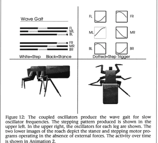
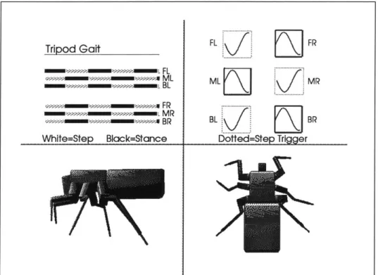
Wilson made hypotheses about the neurological mechanisms which could gen-erate these rules, and his ideas were confirmed by the experimental work of Pearson [28]. Each leg in the cockroach has a pacemaker or oscillator, which rhythmically triggers the leg to step. The oscillators are coupled together, and their interaction generates the various gaits. At slow oscillator frequencies, slow "wave" gaits are generated, and at high frequencies faster wave gaits and the "tripod" gait is generated. As the oscillator frequencies smoothly change, a smooth gait change is effected. The concept of coupled oscillators is not a new one; in the 1930's, von Holst proposed the coupled oscillator model to explain the wide range of interacting cyclic behaviors he observed in nature [29].

In addition to the coupled oscillators, reflexes also play an important role in gait generation. Reflexes can both trigger or retard the

stepping of limbs [28]. In the cockroach, the step

re-flex

causes a leg to step when hair receptors detect that the leg has nearly reached its back-reaching ex-tent. Another cockroach reflex employs cuticle

stress-receptors, which measure the load that a leg is bearing, and prevent a leg from stepping if it is

(18)

sup-porting the insect. In general, reflexes reinforce the stepping pattern generated

by the coupled oscillators, while increasing the adaptability of the creature

under changing environmental conditions. Reflexes seem to play an even more important role during locomotion over uneven terrain. A study by Pearson of locusts walking over uneven terrain shows that a rigid gait is not employed over rough terrain [30]. To find suitable footholds, the legs employ searching tactics, and an elevator reflex causes the leg to lift higher if it encounters an obstacle dur-ing a steppdur-ing movement.

In order to synthesize gait for walking robots or simulations, researchers have created the field of computational gait. McGhee [31] derived the following for-mula which describes the number of distinct gait patterns possible for a k-legged system:

N = (2k - 1)! Equation 1

For a quadruped, therefore, 7! = 5040 distinct gait patterns are possible. For a hexapod, 11! = 3,916,800 gaits can be generated. Selecting which gait to use

from this large number can seem overwhelming. Using a matrix analysis of gait, however, McGhee and Jain showed that the 5040 quadruped gaits can be re-duced to 492 temporally equivalent gaits. They further showed that the 492 gaits can be reduced to 45 equivalence classes. Sun employed further matrix transformations to reduce quadruped gaits to 14 equivalence classes [32]. Sun also showed that the 3,916,800 hexapod gaits can be reduced to 148 equiva-lence classes. In addition, all 288 regular symmetric hexapod gaits can be re-duced to 7 equivalence classes.

Many of the methods used to actually generate gaits are based on

finite state

con-trol [31; 24; 33]. Under this method of control, each leg

cycles through a set of states, such as step and stance. Stepping and stance is typically broken down into smaller sets of states such as step up and forward, and step down and forward.

Communication between the individual leg state machines, and commands from higher levels of

(19)

control determine the stepping pattern.

Beer, Chiel and Sterling employ a heterogeneous neural network to simulate the stepping patterns exhibited by the cockroach [34; 35]. The network is created by a set of coupled differential equations, which model a neuron cell membrane. The cell membrane acts as a resistor-capacitor circuit and sums the input potentials, generating an output frequency. The gait generator employs 37 neurons .For each of the six legs there are three motor neurons, two sensory neurons and one pacemaker neuron. Overall walking speed is set by one command neuron. By varying the firing frequency of the command neuron, a variety of gaits is gener-ated by the network. Slow walking speeds employ the wave gait, and the high-est speed employs the tripod gait, the same behavior exhibited by many insects.

2.3. Motor Control

Once the overall pattern of step and stance sequencing has been coordinated, it must be performed in some manner. In a kinematic simulation, the geometry of the desired motions alone determines the movements. In a forward dynamic simulation, however, forces must be delivered to the limbs to create the move-ments. The problem of dynamic motor control is determining what forces need to be supplied over time in order to create a specified motion. For the fine con-trol of motion, exact forces are required. These forces can be difficult to com-pute, due in part to the forces introduced by the interaction of the different linkages and joints in an articulated figure. For a broader scope of motion, such as "swing leg up and forward," less demanding methods can be employed. In biological systems, the basic producer of

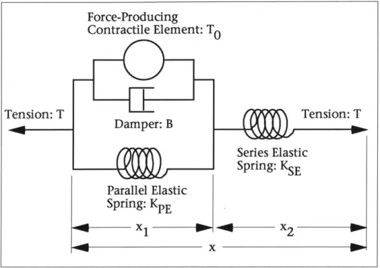
bio-me-chanical forces is the muscle. McMahon [36] con-tains an excellent review of the force-producing properties of muscle, under varying types of stimu-lation. In 1922, V. A. Hill proposed a mechanical model for the active muscle which is depicted in Figure 2. Hill's model is based on a contractile

(20)

ele-Figure 2: The Hill model for the force response of the active muscle.

ment which consists of a force generator in parallel with a non-linear damper. The damper exerts a force as a function of the velocity of muscle shortening

(X1). The contractile element exerts a force, To, as a function of the contractile

element length, x1, and time, t. The contractile force rises and falls with the

muscle stimulation, and during tetanus (the highest efficiency of stimulation and force development) the force To rises to a constant level, equal to the iso-metric tension on the muscle. In addition, a spring in parallel with the contrac-tile element exerts a force as a function of x1. Another spring lies in series with the contractile element and parallel spring, and produces a force as a function of the length x2. The parallel spring models the

elas-tic properties of the muscle fibers, while the series spring models the elastic properties of the

connec-tive tendon. The Hill model has proven very useful

in describing the mechanical properties of muscle acting under a load in the skeletal system. In some

(21)

the diagram in Figure 2, one would be led to believe that a mechanical damper, such as the viscous water medium in the muscle, is acting as a dashpot. In fact, the mechanical properties of the muscle's water does not match the damping ef-fects seen in the Hill Model. The Hill model explains the muscle's force response in mechanical terms, however, it should be noted that muscle is more

accurate-ly modeled as biochemical reactions which release energy.

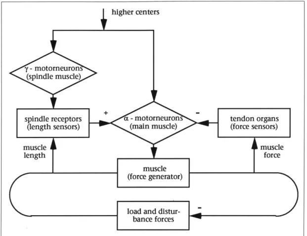
Reflexes and feedback are used to regulate the action of the muscle [36]. The

stretch reflex increases the amount of stimulation a muscle receives when it is

stretched beyond its equilibrium length, as an attempt to return the muscle to its previous length. This reflex is initiated by the muscle spindle organ, which lies in parallel with the main muscle fibers. Within the spindle organ lies a small set of muscle fibers, and a nuclear bag fiber which detects changes in length. When the muscle is stretched by some outside force, the spindle organ senses the change in length and increases stimulation to the muscle fibers. During voluntary movements, the muscle fibers in the spindle organ are co-stimulated with the main muscle mass, from higher centers. This keeps the muscle and spindle organ at approximately the same length, so that the stretch reflex does not interfere with a stretch controlled by higher centers.

Sensors in the tendon organs are responsible for reflex stiffness. The sensors measure muscle force, and send inhibitory signals to the muscles. It is thought that this reflex allows the skeletal-muscular system to present a constant stiff-ness to the world, in spite of changing environmental conditions. A balance is achieved between the spindle organ and tendon organ signals, so that neither length nor force regulation has complete control of the muscle system

(see Figure 3). The tendon organs are also responsi-ble for the clasp-knife reflex. This reflex prevents the muscle from over-exerting itself and causing dam-age to tissues. The force sensors in the tendon organ detect strong force and send strong inhibitory sig-nals to the muscle. When the reflex becomes active, the limb it controls suddenly looses tension, which

(22)

Figure 3: A diagram of stiffness regulation in the stretch reflex [361. looks somewhat like a clasp-knife returning to its sheath.

Starting with the assumption that muscles are tunable, spring-like force genera-tors, motor control researchers have come up with an equilibrium-point

hypothe-sis to explain how controlled movements are produced [37; 38; 39; 40]. This model

treats the muscle, along with its feedback system, as a single, tunable unit, with measurable, spring-like properties. Postures are controlled by establishing an equilibrium between agonist and antagonist muscle

groups. This equilibrium configuration forms a point in a controlling space, which can be specified

by the neuromuscular system. The

equilibrium-point hypothesis states that movements are pro-duced by changing the equilibrium point from one posture to another. Exactly how the change from

(23)

one point to another is accomplished is not fully understood. Experiments by Bizzi, Chapple and Hogan show that it is not the case that the equilibrium point is instantly switched from one point to another [37]. Hogan describes a "virtual trajectory" of equilibrium points which control movements[39].

One of the basic controlling means in nature is the servomechanism [20], which employs negative feedback to steer a system toward some equilibrium. Sensors are used to measure some signal, and an error term is constructed based on the displacement of the system from its goal. The error term is used to stimulate the system in the direction of the goal. The way in which moths orient towards the light is a servomechanism; unless both eyes detect light, the moth turns more towards the light. If one eye of a moth is blinded, it turns continually in a cir-cle, since only one eye is ever illuminated. The controlling means of the stretch reflex, described above, can also be thought of as a servomechanism, since it employs active feedback to regulate the length of the muscle system.

The study of computational motor control has arisen mostly from the need to con-trol robotic systems. Again, the problem comes down to what forces are

re-quired to produce specific motions. In many cases, the demands on precision can be very high. In some applications, not only the motion of the system needs to be controlled, but also the force applied by the robot onto its environ-ment.

Before describing computational motor control, an interesting example of

inter-active motor control will be presented. An interinter-active graphical editor, Virya,

de-veloped by Wilhelms, allows controlling functions to be specified for an articu-lated figure simulator [41]. The user draws and edits

curves to indicate what forces or torques are to be applied at a degree of freedom. Alternately, the

mo-tion of the degree of freedom can be defined with a ... curve, and an approximate force will be

automati-cally calculated to achieve approximately that mo-tion. Results from using Virya and similar

(24)

experi-Figure 4: a simple servomechanism implementing spring position control

ments by Armstrong, Green and Lake [13], reveal that direct manipulation of the forces and torques needed to achieve certain motions or goals is very difficult. One problem is that there are typically many degrees of freedom to control. Another problem is that forces applied at one degree of freedom influence not only that DOF, but also (potentially) the entire dynamic system. In addition, Coriolis and centripetal forces arise due to the motion of the bodies in the sys-tem, and must be counteracted for accurate motion.

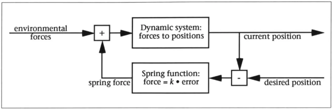
A basic servomechanism might be used to automate motion control. A simple

feedback system which employs a spring to draw a dynamic system towards a specified position is shown in Figure 4. A linear spring function produces a force proportional to the displacement of the dynamic system from the target posi-tion. The feedback system will automatically respond to external perturbations which cause a drifting from the target. The problem with this basic approach is

that the system will not necessarily ever reach the target. Once an equilibrium is reached between the spring force and external forces, the spring cannot draw the system any closer to the goal. Increasing the

spring strength, k, will make the error displacement smaller and smaller, but not zero. In addition, the simple spring system depicted in Figure 4, in the ab-sence of damping (from external forces), will

actual-ly fight itself; the spring will bring the system closer

(25)

up momentum and overshoot the target. The spring will then have to pull the system back again, and so on.

Inverse dynamic techniques (including constraint based systems) can calculate the exact force required to bring the system to a target, without any displace-ment. However, in order to exactly counteract external disturbance forces, those forces must be known. In a simulation system, it is reasonable to say that these forces will be known, but it is not always a valid assumption that the controller should have knowledge of them. For example, if a simulated human was stand-ing and received a push from the side, the controllstand-ing system should not know exactly what force is being applied and immediately counteract it, if a humanly-realistic motion is desired. Instead the human should begin to fall to the side, and when the controller discovers the error in balance, it would try to correct and rebalance.

An, Atkeson and Hollerbach employ model-based control [42], in which a descrip-tive model of the kinematics, dynamics and motors of a system are used to com-pute accurate controlling forces for robot manipulators. The complete robot sys-tem, including motor properties, linkage elasticity, joint viscosity, etc., is often termed the plant. A model of the inverse-plant is used to predict and plan how the system will respond to controlling input. Determining the exact values for a plant, and thus its inverse, can be difficult, however.

Another class of inverse-dynamics controlling methodologies are optimization

techniques. With these techniques, a goal is specified, along with the details of

the physical system. Some measurable quantity, such as energy expenditure, is chosen to be minimized. The system is then

ana-lyzed over a period of time to determine what con-trolling parameters will yield the optimal result. Because optimization techniques solve the entire dynamic system with controlling parameters over an interval of time, they can be quite computation-ally expensive. Brotman and Netravali have

(26)

devel-oped a system using optimal control to interpolate between a set of motion key-frames [43]. Witkin and Kass term their method of optimal control spacetime

con-straints [9]. Their method allows goals to be specified in kinematic and energy terms, such as "jump from here to there, clearing a hurdle in between, and don't waste energy."

Optimization techniques along with other constraint techniques can be termed

key event simulation, because specific events must be satisfied. This is in contrast to forward simulation in which a system is established, and then simulated

for-ward in time [44]. Controlling techniques for key event simulation require glo-bal knowledge about the system, sometimes over the entire time span of the simulation. Forward simulation controllers, however, need only partial knowl-edge of the world, presumably derived from a simulated sensor. The more so-phisticated the controller, the more knowledge of the world it will require. External influences, such as interactive input, can be easily incorporated into a forward simulation at any point in time, unlike methods such as spacetime con-straints, which must be solved over the entire span of time.

2.4. Walking Machines and Simulations

Walking machines have been the subject of research for many years. A human-controlled, four-legged vehicle was developed at General Electric by Liston and Moser in the mid-1960 [45]. Using force-feedback, the driver could "feel" obsta-cles and negotiate uneven terrain. The first example of an autonomous legged vehicle, controlled by a digital computer, was a hexapod robot developed by McGhee [46]. The hexapod could employ a number of gaits, and negotiate rough

terrain with areas marked as forbidden. A similar hexapod was developed by Sutherland [47]. Its gait control system is similar to

the one presented in this thesis [24]. Legged robots designed by Raibert differ from the above robots in that they employ dynamic balance; i.e. they can run and hop without enough legs always on the ground to statically support the body [48].

(27)

In the computer graphics field, simulations of legged locomotion have also been an area of active research. A kinematic simulation of human walking was devel-oped by Zeltzer using a finite state machine approach [33]. The biped model was capable of walking over uneven terrain. However, since the motions lacked a physical basis, some of the walking appeared overly simplified, especially when adapting to terrain. Girard developed a system for kinematically simulating the locomotion of creatures with various numbers of legs [49]. In his system, gaits and leg motions are interactively created, and gait shifts are accomplished by simply interpolating between defined gaits. Some dynamic aspects were also added, such as parabolic trajectories while in the air and banking during turns. However, because the motions are interactively defined, the overall motions lack a complete dynamic basic, which can make them appear artificial. Sims

created a walking system with an interactive figure editor which allows the user to quickly and easily define new figures [50]. The figure can then automatically employ defined gaits over uneven terrain, and also hop or "pronk" using a dy-namic trajectory. A dydy-namic model of snake and worm locomotion was devel-oped by Miller [51]. Although not legged locomotion, Miller's work is interesting in this context because of its dynamic nature. The forward motion of the snakes is ultimately due to friction, as is the motion of the roach in this thesis.

(28)

3. Approach

This chapter describes the approach that I have taken to develop a dynamic model of locomotion. My approach is basically one of forward simulation, where a physically accurate model of a hexapod and its environment is constructed,

and a control algorithm for walking is established (without global knowledge of its environment), and the system is then simulated forward in time. The success or failure of the system depends on the accuracy and robustness of the control system, as the dynamic simulation will faithfully incorporate all controlling forces, whether they help or hinder locomotion.

My approach breaks down into three main procedural components which

de-scribe how the physical and controlling mechanisms will operate, and a set of

structural components which describe the parameters of the hexapod

(see Figure 5). The three procedural components are: a dynamic simulator, a gait controller and motor programs. Dynamic simulation forms the foundation of the system, since all motions are computed by the simulator. Because a forward dynamics simulator is employed, forces must be applied to create movement.

(29)

Featherstone's Articulated Body Method (ABM) [10; 52] was selected as the simu-lation algorithm, because it is one of the most efficient methods for forward dy-namics. The gait controller coordinates the sequences of stepping and stance for the hexapod. The controller used in this thesis is based on the coupled oscil-lator model with reflexive feedback [28]. The motor programs generate the forces required for stepping and stance. They are based on exponential spring and damper combinations, which are tuned over time. In addition, there is another procedural unit, the graphics system, which is not directly involved in the

cre-ation of locomotion, but is required for display and animcre-ation of the simula-tion.

The structural components describe the parameters that the functional units will operate on. The structural model of the hexapod describes how it mechani-cally constructed (i.e. the kinematic structure of the links and joints, and the mass and inertia of the links), how it appears when graphically rendered, and the specifics of how it will move (i.e. the maximum speed, motor program pa-rameters, etc.) Some of the structural elements were designed from a study of

in-sect physiology, others were developed by trial and error methods. 3.1. Dynamic Simulation

As has been previously noted, the dynamic simulator forms the basis of all mo-tion in this dynamic locomomo-tion system. The simulator accepts forces acting on an articulated body as input, and computes the acceleration of the degrees of freedom of the figure as output. These accelerations are numerically integrated over time to give rise to the velocities and position of the DOF's.

Featherstone's ABM is introduced in [52], and developed further in [10].

Featherstone claims (with substantial proof) that the ABM is the most efficient algorithm yet developed for forward dynamics simulation. Deyo and

Ingebretsen [53] claim that Bae's recursive algorithm [54] is the most efficient, al-though the claim is not substantiated. The main reason for the algorithm's effi-ciency is because it is recursive in nature. Instead of solving a set of simulta-neous equations describing the kinematic and dynamic relationships between

(30)

different links in an articulated figure, recursive dynamics formulations estab-lish a recursive, linear relationship between parent and child links. The simulta-neous equations methods have a computational complexity of approximately

O(n3), whereas recursive methods can achieve a complexity of 0(n), as the ABM

does.

The ABM operates on branching, articulated figures, comprised of links connect-ed by joints. The joint type in the ABM is flexible in that many different joint types can be specified. For example, rotary and prismatic (translational) joints

are supported, as well as combinations of both, such as screw and cylindrical joints. A joint can have from one to six degrees of freedom.

One of the links in the articulated figure is chosen to be the root body, or base. This link can actually be any of the links in the figure, but it is logical to choose the most central body in the branching structure. If the recursive algorithm were implemented on a parallel processor machine, then the most efficient root body would be the most central, since all branches could be processed in paral-lel. The root body is somewhat special in the ABM since kinematic constraints

can be specified for it. The other links in the figure, including the end-effectors (last link in a branch of the figure), do not support kinematic constraints; their motion is determined by the applied forces only. However, an inverse dynamics algorithm can be used to compute those forces needed for kinematic

con-straints.

The key feature of the Articulated Body Method is the concept of the articulated body inertia. Just as the inertia tensor of a rigid body determines its acceleration when the applied force is known, the articulated body inertia tensor of a rigid body, within an articulated figure, determines the acceleration when the ap-plied force is known. Formally, the equation of motion for a free rigid body is:

f =

I

a + p Equation 2

where f is the applied force, I is the inertia tensor, a is the acceleration and p, is the bias force (centripetal and Coriolis) produced by the body's velocity. The

(31)

equation of motion for rigid body gantry motion in an articulated figure reads:

^ ^A

,,.'-f =

I

a + p Equation 3

^A

where I is the articulated body in-ertia tensor, and p is the bias force

which incorporates the pV from block m

motion above, as well as joint reaction

forces. The ^ above these

quantities denote that they are rep-resented in spatial notation. This

notation, developed by x

Featherstone, is based on screw Figure 6: a two dimensional block and gantry calculus [55], and essentially unites

the rotational and translational aspects of motion into a single vector quantity. Appendix A gives an introduction to the spatial algebra required to implement the ABM, however, Featherstone should be referred to in [10] for a tutorial in and reference for spatial notation.

"A

The articulated body inertia ( I ) gives directional properties to the apparent mass of a body. To use an example from Featherstone [52], a simple two dimen-sional block and gantry system will be described (see Figure 6). The first mass,

mi1, is a block free to move up and down in y along the second mass, m₂, to

which it is attached by a prismatic joint. The second mass is free to move from side to side in x along another prismatic joint. A force applied to n1 in the y

di-rection will yield an acceleration in the y:

a =-Equation 4.

A force applied to mi or m2 in the x direction, however, needs to overcome the

(32)

ax = mi+m _{Equation 5.} These two equations can be combined into a single matrix equation:

fy7

0

1 .ami

Equation 6.

It can be seen that the apparent mass of the system is higher in the x direction than in the y. It is the difference in the degrees of freedom between the two bodies due to the joints which creates this effect. The mass matrix in Equation 6 is the articulated body inertia for this two dimensional system.

The full development of the ABM is left to Featherstone [10], however, the basic equations needed to implement the ABM are described in Appendix B. The basic operation of the algorithm progresses as follows: first the algorithm passes

from the leaf bodies of the figure tree in to the root body, accumulating the ar-ticulated body inertia (IA ) and bias forces (

p),

then Equation 3 is used to com-pute the acceleration of the root body as in:

a= (IA) (f - P) Equation 7

finally, the algorithm passes from the root out to the leaves computing the ac-celerations of the joints.

3.2. Gait Control

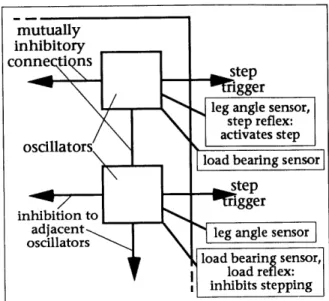
In order to coordinate the stepping and stance of the hexapod, a biologically-in-spired approach has been used. A computational model of coupled oscillators is used to generated the overall stepping patterns. In addition, feedback via reflex-es reinforcreflex-es the general stepping pattern while increasing the adaptability of the gait. The coupled oscillator model is employed in this thesis because it is adaptive and robust, and because it lends itself well to hierarchical structuring. The higher centers of control simply specify walking speed, and the gait con-troller selects the appropriate gait, and sends motor commands to the levels below it.

(33)

an action. Each leg receives an

os-cillator, and the action which it oscillators

triggers is stepping. The coupling step triggers

between oscillators will be mod-eled as phase and time

relation-ship rules which the oscillators master

maintain between each other. oscillator les

These relationships are mathemat-ical translations of the stepping

rules observed in the cockroach abdomen

by Wilson, presented in the

Background and Related Work

chapter. The oscillators cycle with Figure 7: the coupled oscillator configuration the same frequency, such that a

master frequency is set, and all oscillators match that frequency (see Figure 7). Because of the coupling rules between oscillators (most importantly, that legs across from each other step 1800 out of phase) different gaits and walking

speeds result when the oscillator frequency is varied. Further details of these models will be given in the Implementation chapter.

Reflexes are modeled as conditional units. When a certain condition is met, the reflex can inhibit or trigger different actions. For example, the step reflex trig-gers stepping when a leg is bent back past a specified angle. This helps the hexa-pod avoid over-extending the reach of its legs. An inhibitory reflex prevents stepping if an immediate neighbor (front, back and side) of a leg is already step-ping. In general, adjacent legs should not step simultaneously, since it would decrease the stability of the supporting legs. An exception to this rule is seen in the locust when negotiating uneven terrain [30]. The two middle legs of the lo-cust are lifted simultaneously, while the other legs support, in order to lift the legs out of a large depression in the terrain. A load bearing reflex inhibits step-ping if a leg is currently bearing too much weight (see Figure 8). This prevents the hexapod from stepping with a leg that is currently an important support

site. Again, more details on the models will be presented in the

(34)

Implementation chapter.

connIt should be noted that this

mod-rigger _{eling is not a fine-grained neural}

leg angle sensor,

step reflex: network approach as Beer, et al,

oscillatorshave employed [34]. Instead, the

loadoscillators

and reflexes are mod-ger

inhibitiongger eled as computational units, and

adjacent leg angle sensor the oscillator coupling is modeled

oscillators

load beari as rules for the oscillators units to

loadr ex:

eiinhibits stepping follow.

Figure 8: reflex feedback to the oscillators The oscillators and reflexes trigger

the stepping motor programs for the legs. One stepping is initiated, it continues to completion and stance begins again. The gait controller only generates the pattern of stepping, and is not directly responsible for the movements of the legs or body. However, the movements of the legs, due to the motor programs

and dynamic simulation, do feedback into the gait controller through the re-flexes.

3.3. Motor Programs

The dynamic motor programs are responsible for delivering forces, through the joints of the hexapod, to create the movements required for locomotion. There are two motor programs: step and stance. The stepping program must compute the forces necessary to lift the leg up and forward, and place it in a position to take up the load of the body when stance begins. The stance program supplies the forces needed to support the body via the legs, and propel it forward. Stepping programs are triggered by the gait controller, as described above.

Stance programs automatically begin when stepping has completed.

The dynamic motor programs create forces by using exponential springs. As their name implies, These springs have an exponential relationship between the displacement, x, of the spring from its rest position (or angle) and the force

(35)

f (force)

generated, f, such that:

f = a (eiA - 1) Equation8 400

where a controls linear strength, 300

and

p

controls exponential rise. The

force response of an exponential 100

spring is shown in Figure 9. The ex-..

-2 -11 2

ponential response creates a steep The effect of varying 0: a=1; V- 4, 3,2

potential well; with a large displace- f 3 torce)

ment, the force becomes extremely

high. The

p

parameter controls the 250

C-200

width of the well, and the a

param-eter controls how fast a well of a 100

given width will linearly rise. When 50

an exponential spring is used for po- 2 1 2

sition control, the degree of free- The effect of varying a: a--2 1 0.S; -3

dom it controls will very likely stay Figure 9 the force response of an

within the lower parts of the well, exponential spring: f (e1A - 1)

since the forces grow so large out-side of the lower region.

A motor program controls motion by changing the rest position (or angle) of its

exponential spring over time. This causes the force potential-well to travel along the degree of freedom, "dragging" the controlled limb along with it. The rest position is modified using a linear interpolation from the current position to the target position. In more physical terms, the rest position travels with a con-stant velocity to the target. This is not an exacting method of motion control, and would be inappropriate for a movement such as a controlled reach and grasp.

Although this springy method of motor control does not allow specified trajec-tories to be exactly executed, it does have an interesting advantage over

(36)

meth-ods which do control exact move- z (torce)

400-ments (especially kinematic systems).

The potential wells created by the 300

springs lead to a compliant system, 200

which allows the final motion to fall

within a range of possible motions. 100

For example, to negotiate uneven

ter-rain, a kinematic locomotion system 2 1

would need to compute the leg joint Figure 10: linear vs. exponential spring force angles needed to place a foot at

differ-ent heights at differdiffer-ent points on the

terrain. Using a dynamic, compliant system however, the legs can automatically adjust to the different heights of the terrain, which is demonstrated in this the-sis. For example, if a foot were to land in a hole, the joint angles would be rotat-ed beyond their normal values, but would still fall within the force potential well created by the springs. When a foot lands on a rise, the joint angles would be compressed more than usual, but the compliant response in the joints would

allow this. In the hill case, the force response of the springs would lie on the op-posite side of the potential well from the hole case.

A disadvantage of using exponential springs is that they create a stiff system. As

the force response of the springs is pushed further and further up the steep walls of the potential well, the numerical sampling of the integrator must take small-er and smallsmall-er time steps to get an accurate result. Linear springs would not cre-ate such a stiff system for a given force output, but exponential springs have the advantage that at small displacements, they are less stiff than linear springs (see Figure 10). In addition, linear springs need to be very strong to create simi-lar forces to the exponential springs at simi-large displacements.

In some basic structural ways, this method of motor control is similar to the equilibrium position hypothesis, presented in the Background and Related Work chapter. I am not claiming to model that hypothesis, but rather claim that the gross hierarchical structuring is comparable. In the equilibrium

(37)

posi-tion hypothesis, moposi-tion is created by "interpolating," in some manner, between different postures. This interpolation occurs in a neuromuscular controlling

space. In my dynamic motor program model, different postures are "calibrated" (discussed in the Implementation and Results and Analysis chapters) and mo-tion is achieved by interpolating between them. The controlling space of the motor programs is the rest length of the exponential-spring actuators.

3.4. Roach Description

The final component necessary for a simulation of dynamic locomotion is the set of data needed to describe the hexapod/roach model. This model includes not only the graphical objects used for display, but also other information specifying the mechanical design of the articulated figure, as well as data de-scribing how the roach will walk. Essentially this data is a set of static informa-tion which describes the physical properties, control parameters and graphical models for the hexapod. All of this data will be detailed in the Implementation

chapter.

The physical properties include the size, shape and density (and thus mass and inertia) of each link in the figure, as well as the figure's mechanical design. The mechanical design describes how the figure is constructed: the joint axes' loca-tions, directions and degrees of freedom, and the branching tree structure of the figure. This kinematic design is based on studies of cockroach physiology, from diagrams and text descriptions [22; 56].

The control parameters determine the basic gait features and the motor program parameters. Constant gait features are the stepping speed, the time between

stepping of adjacent legs on the same side of the body, the number of legs and default values for other parameters such as oscillator frequency. The motor pro-grams for step and stance define what joint angles are traversed by the exponen-tial springs during those actions. These programs are "tuned" via a trial-and-er-ror method to determine appropriate spring strengths and joint angle values. In general, this trial-and-error approach is not the appropriate method to deter-mine the operating dynamic parameters, since it requires an "expert" tuner (i.e.

(38)

the programmer) to make "educated" guesses as to the parameters, based on the experience gained from previous experiments. In some sense, the expert tuner acts as natural selection in an "evolutionary" process which increases the ro-bustness of the locomotion. Other methods for determining the motor parame-ters will be discussed in the Future Work section.

The same data that is used for the computation of the physical inertia (the size and shape of the body parts) is used as the geometric data for graphical render-ing. In addition, rendering information such as the color, shading parameters and lighting models is specified for all of the graphical objects.

(39)

4. Implementation: Corpus

In order to implement the methods described in the Approach chapter, the program corpus was designed and programmed by the author. Corpus is a system for simulating the forward dynamics of articulated figures, with gait control mechanisms, force-producing motor programs and rendering support. A "corpus" is the body of a man or animal (Webster's 7th), and thus the

articulated-figure simulator, corpus is so-named. Corpus is implemented in the c programming language, and uses several support libraries, also implemented in

c: rendermatic (David Chen, MIT), a rendering library with geometric collision

detection; retepmatic (Peter Schr6der, MIT), additional rendering code; and

robotlib (David Chen, MIT), a matrix manipulation package. The control of corpus is implemented through a scripting command language, which allows

figures to be constructed, dynamically simulated, gait controlled, motor controlled and rendered.

The data which describes the mechanical structure of the hexapod and the spe-cifics of how the hexapod will walk (gait and motor parameters) form the re-maining parts of the implementation of this thesis. Although not directly a part

of corpus, this data describes the operating parameters for the program

execu-tion.

4.1. Dynamic Simulation

Corpus employs the Articulated Body Method (ABM) described in the Approach

chapter and Appendix B. Underlying the ABM is a set of spatial algebra

functions (see Appendix A for a discussion of spatial algebra). These functions include:

" spatial operators (e.g. spatial transpose, spatial cross), " spatial transformation matrix operators,

e and operators used to build spatial quantities from more intuitive data and to recover that data from spatial quantities.