Analytical model for RF power performance of deeply scaled CMOS devices

Analytical model for RF power performance

of deeply scaled CMOS devices

The MIT Faculty has made this article openly available.

Please share

how this access benefits you. Your story matters.

Citation

Gogineni, Usha, Jesus del Alamo, and Alberto Valdes-Garcia.

“Analytical Model for RF Power Performance of Deeply Scaled CMOS

Devices.” IEEE Radio Frequency Integrated Circuits Symposium,

2011. 2011 1–4.

As Published

http://dx.doi.org/10.1109/RFIC.2011.5940647

Publisher

Institute of Electrical and Electronics Engineers (IEEE)

Version

Author's final manuscript

Citable link

http://hdl.handle.net/1721.1/71960

Terms of Use

Creative Commons Attribution-Noncommercial-Share Alike 3.0

Detailed Terms

http://creativecommons.org/licenses/by-nc-sa/3.0/

Analytical Model for RF Power Performance

of Deeply Scaled CMOS Devices

Usha Gogineni

, Jesús del Alamo

, and Alberto Valdes-Garcia

1

Massachusetts Institute of Technology, Cambridge, MA,

IBM T.J. Watson Research Center

Abstract — This paper presents a first order model for RF

power of deeply scaled CMOS. The model highlights the role of device on-resistance in determining the maximum RF power. We show excellent agreement between the model and the measured data on 45 nm CMOS devices across a wide range of device widths, under both maximum output power and maximum PAE conditions. The model allows circuit designers to quickly estimate the power and efficiency of a device layout without need for complicated compact models or simulations.

Index Terms — CMOS, power amplifiers, millimeter wave,

on-resistance, PAE.

I. INTRODUCTION

Estimating the maximum RF output power for a device at any given bias point is an onerous task. Power amplifier designers often rely on RF power simulations using compact device models [1-2]. These simulations are very time consuming and the need for accurate compact models means that the power estimations are only accurate when designing in mature device technologies. Moreover, in the case of CMOS, compact models are usually tailored for digital or analog applications and hence are not accurate enough for modeling the device behavior under the large signal swings characteristic of RF power applications. Also, power simulations around the peak PAE point often lead to convergence issues and hence do not predict the peak power very well [3].

In view of all the challenges described above, it would be ideal to have a simple analytical model that can predict the maximum output power and the trade-off between output power and PAE in a device. The analytical models presented in textbooks [4-10] usually ignore Ron and also assume zero VDSsat. However, to obtain high power, the device is usually biased at a high drain current, which means the output power is strongly affected by Ron. In this paper, we present an analytical model that correctly accounts for the on-resistance of the device, thus allowing us to make quick back-of-the-envelope predictions of the output power and PAE. We validate the model by comparing the power and efficiency predictions from the model with measured load-pull data on 45 nm CMOS devices.

II. MODEL DESCRIPTION

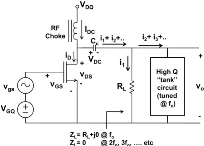
The power amplifier model used in this paper is based on the overdriven class AB amplifier discussed in [4] (Fig.

1). The transistor is characterized by a threshold voltage Vt and an on-resistance Ron. It is biased at an operating point (VGQ, VDQ). The current through the drain in the absence of RF input signal is IDQ. The RF load consists of a fundamental load resistor RL, and a shunt connected “tank” circuit with its resonant frequency at the fundamental frequency of operation (fo). All harmonics in the load current are assumed to be shorted by the tank circuit and generate no voltage. Hence, the current flowing through RL is just the first harmonic, i1, and the voltage across RL is assumed to be sinusoidal with a magnitude set by the load resistor.

Fig. 1: Circuit diagram of a reduced conduction angle RF power amplifier.

Fig. 2: Waveforms for input voltage and output current and voltage in the reduced conduction angle amplifier of Fig. 1.

VDQ IDC VDC VGQ vgs vGS vDS RL Cc RF Choke + + + -- vo + -ZL= RL+j0 @ fo ZL= 0 @ 2fo, 3fo, …. etc iD i1+ i2+.. i2+ i3+.. i1 High Q “tank” circuit (tuned @ fo)

Fig. 2 shows the waveforms for key voltages and currents in the power amplifier when operated in the maximum power condition for a certain bias point and load resistance. When vGS < Vt, the device enters the cut-off regime and the drain current is zero. When vGS > VGSsat, the device enters the linear regime and the drain current is clipped at Iknee. For all other values of vGS, the drain current is assumed to be cosinusoidal. The shape of the drain voltage waveform is 180 degrees out of phase with the drain current waveform. When iD = Iknee, vDS is pinned at the minimum value Vmin, and when iD = 0, the drain voltage is clipped at Vmax.

α denotes the conduction angle and represents the proportion of the RF cycle for which vGS > Vt and iD > 0. Since the waveform is symmetric about ωt = 0, the current cut-off points are at ωt = ±α/2. β denotes the proportion of the RF cycle for which vGS > VGSsat and iD = Iknee.

Assuming that the drain current and voltage follow a pure cosine between α/2 and β/2, we can write:

0 | | 2 cos 2 | | 2 0 2 | | (1) 0 | | 2 cos 2 | | 2 2 | | (2)

The values of Iknee, Id, Vo and Vd can be determined by recognizing that the waveforms need to be continuous at α/2 and β/2.

Vmin can be expressed in terms of Iknee and Ron as: (3) Our model describes the maximum power situation for any given value of α and β. Hence, we assume a maximum voltage swing for vDS that is symmetric about VDQ. In other words,

2 (4)

This assumption is widely made in the analysis of power amplifiers [4, 6, 8].

The magnitudes of the DC and fundamental component of the drain current and voltage can be obtained by Fourier analysis of equations (1) and (2):

cos 2 2 cos2 cos2 2 cos2 sin2 sin2

(5) 2

cos 2 sin2 cos2 cos2

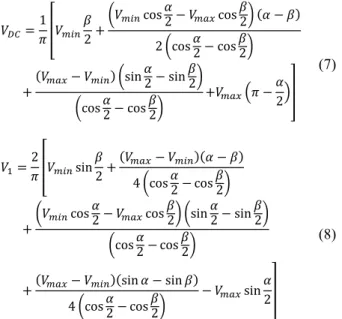
sin sin 4 cos 2 sin2 sin2 4 (6) 1 2 cos 2 cos 2 2 cos 2 cos 2 sin 2 sin 2 cos 2 cos 2 2 (7) 2 sin 2 4 cos 2 cos 2

cos 2 cos 2 sin 2 sin 2

cos 2 cos 2

sin sin

4 cos 2 cos 2 sin2

(8)

The fundamental component of the drain voltage is the same as the voltage across the load resistor. This is, because we assumed that VDC drops across the capacitor Cc and that the second and higher order harmonics are shorted out at the fundamental frequency of operation.

The output power, efficiency, and fundamental load resistance values that are associated with a particular choice of α and β can then be directly computed using the following expressions:

· (9)

√2·√2 (10)

% 100 (11)

(12) The model equations presented above can be used to generate the drain efficiency – output power locus for any given device. The inputs to the model are the DC operating point (VDQ, IDQ) and Ron of the device. For any given value of α and β, describing a random maximum power condition, the value of output power, drain efficiency, average current and load resistance can be computed using the above expressions. This exercise is repeated for multiple pairs of α and β to construct the drain efficiency – output power locus.

An example is shown in Fig. 3 for a device with Ron = 9.6 Ω biased at VDQ = 1.1 V and IDQ = 200 mA/mm. Ron was calculated from measured DC data as VDS/ID with VDS = 50 mV. For any given α, as β is increased, more of the current waveform gets clipped at Iknee, and more of the voltage waveform gets clipped at Vmin. This leads to a decrease in the peak of the current waveform and a corresponding increase in the peak of the voltage waveform. In turn, this results in a decrease in IDC and I1 and a corresponding increase in VDC and V1. Since Pout =

I1V1/2, as β increases, Pout initially increases because of the rise in V1, but then starts decreasing as the reduction in I1 begins to dominate. On the other hand, since IDC decreases with increasing β, the drain efficiency increases monotonically. As α decreases towards class B operation (α = π), the peak of the current waveform increases, thus leading to higher power.

Fig. 3: Modeled locus of drain efficiency versus output power. Pout and ηD measurements at different RL are shown as symbols in

the figure and show good agreement with the model. III. COMPARISON WITH MEASUREMENTS The devices used in this study were fabricated using IBM’s 45 nm low-power CMOS process [11]. The test devices have a gate length of 40 nm and are designed to operate at VDD=1.1 V. Devices with gate widths between 40 μm and 640 μm were fabricated by connecting multiple unit cells in parallel. Each unit cell contains 20 fingers of 2 μm finger width. RF power measurements were performed in the 2 – 18 GHz range using a Maury Microwave load-pull system. Power measurements for all devices were performed at VDS = VDD, and VGS set to yield a DC drain current density IDQ = 200 mA/mm under low input power conditions. The output power and PAE were recorded at an input power level corresponding to the peak PAE condition. The source and load impedances were tuned for either (a) maximum Pout, or (b) maximum PAE. fmax for these devices, at the bias point under consideration, ranged from 200 GHz in the narrow devices to 100 GHz in the widest device. We found that the output power measured on the 45 nm devices is independent of frequency in the 2-18 GHz range [12]. Therefore, for f << fmax, the frequency dependence is smaller than the influence of other factors, and hence has been ignored in this work.

The RF power data measured on a W = 40 μm device at several RL values is shown along with the model data in Fig. 3. The measured data shows reasonable agreement with the modeled locus.

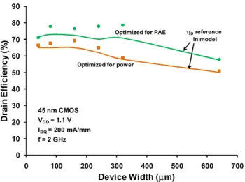
The modeled ηD – Pout locus can be used to predict the maximum output power a device can deliver at a given drain efficiency, or vice versa. Fig. 4 shows the measured ηD (symbols) and the values chosen as input to the model (solid lines) for the two different impedance matching conditions (optimized power and optimized PAE). The

appropriate Ron and DC operating points were used in the model for each device.

Fig. 4: Drain Efficiency as a function of device width. The solid line represents ηD selected as reference in the model for

predicting maximum Pout and optimum RL for that ηD. The

symbols are the measured _ηD at 2 GHz.

The model assumes that only the first harmonic of the drain current flows through the load resistance and that all the other harmonics are shorted out through perfect impedance matching at the fundamental frequency. However, in practice the impedance match need not be perfect and could yield non-zero values of second and higher order harmonics of the current. This would result in an increased value of the output power and drain efficiency. This explains why the maximum modeled drain efficiency was less than the measured values for some of the devices. In such cases, the maximum modeled efficiency closest to the measured value was selected as input to calculate the maximum Pout.

Fig. 5: Output power as a function of device width. The solid line represents the maximum Pout predicted by the model. The symbols

show the measured Pout at 2 GHz.

For each value of drain efficiency chosen as input, the maximum possible power predicted by the model, for any combination of α and β values, is recorded. The corresponding values of alpha and beta are also noted and are used to calculate the average drain current and the load resistance. 0 10 20 30 40 50 60 70 80 90 0 100 200 300 400 500 600 700 D rai n E ff ici en cy (% ) Device Width (μm) 45 nm CMOS VDD= 1.1 V IDQ= 200 mA/mm f = 2 GHz

Optimized for PAE

Optimized for power

ηDreference in model 0 10 20 30 40 50 60 70 80 0 100 200 300 400 500 600 700 Ou tp u t Po w er ( m W ) Device Width (μm) VDD= 1.1 V IDQ= 200 mA/mm f = 2 GHz

Optimized for PAE Optimized for power

model output 45 nm CMOS W = 40 μm β = 0 β = π α=190 α=200 α=210 α=220 α=240 α=260 α=290 α=360 α=320 VDQ = 1.1 V IDQ = 200 mA/mm Ron = 9.6 Ω

Fig. 5 shows the modeled values for maximum output power and the measured data, across all device widths. The excellent agreement suggests that the maximum output power delivered by a device at any given bias point is only limited by the on-resistance of the device. The device capacitances play a role in degrading the PAE of the device. However, as long as extra input power can be provided to charge the capacitors, one can always obtain the same maximum power.

The measured Pout on the 640 μm device is significantly lower than the modeled value (Fig. 5). This could be because of self-heating effects, which become significant in the wide devices. The self heating explanation is further borne out in Fig. 6, where the modeled and measured values of the average drain current (IDC) are shown as a function of device width. In general, the modeled IDC closely matches the measured values, thus validating the model. The measured IDC on the 640 μm device is somewhat lower than the modeled value, also consistent with self heating.

Fig. 6: Average drain current as a function of device width. The solid line represents IDC predicted by the model. The symbols

show the measured IDC at 2 GHz.

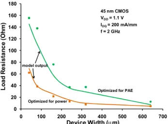
Fig. 7 shows the load resistance used in the power measurements (symbols), as well as the value of RL computed from the model (solid lines). The modeled values show reasonable agreement with the measurements. This means designers can use this model to not only predict the maximum output power of a device for any given drain efficiency, but also to estimate the load resistance needed to achieve the required power. Output matching networks can then be designed to present this resistance to the load.

In a CMOS device, Ron can be approximated as the sum of the source resistance (RS) and drain resistance (RD), since the channel resistance is typically much smaller than RD or RS. Hence, if we can estimate RD and RS for any device layout, through parasitic extractions from layout, we can predict the maximum Pout and ηD for that device. Thus, using this model, circuit designers can estimate the power capability of their designs and optimize the design to achieve the necessary power or efficiency targets.

Fig. 7: Load resistance needed to obtain maximum Pout. Solid line

is optimum RL predicted by model. Symbols are measured data at

2 GHz.

IV. CONCLUSION

A simple analytical model for the RF output power and drain efficiency of CMOS has been presented. The model uses the DC operating point and on-resistance of the device as inputs and gives out the maximum output power and the load resistance at any value of the drain efficiency. We have shown that the modeled values of Pout, ηD, and RL show excellent agreement with the measured data on 45 nm CMOS devices across a wide range of device widths. Our work shows that on-resistance is the most significant limiter to the output power of CMOS devices. Circuit designers can use this model to estimate the power and efficiency of their device and to optimize their device layout to meet performance targets.

ACKNOWLEDGEMENT

This work was funded by a Semiconductor Research Corporation (SRC) grant 2007-HJ-1661. The authors would like to thank IBM Microelectronics for fabricating the test structures.

REFERENCES

[1] S. Aloui, et al., “A 60GHz 13 dBm fully integrated 65 nm RF CMOS power amplifier”, NEWCAS-TAISA, 2008, pp: 237-240. [2] N. Kurita, et al., “60GHz and 80GHz wide band power amplifier MMICs in 90nm CMOS technology”, RFIC, 2009, pp: 39-42.

[3] P. Estrada, “Overcoming verification tool limitations for analog / RF designs”, EE Times Design, 2007.

[4] S. C. Cripps, RF Power Amplifiers for Wireless

Communications, 2006.

[5]B. J. Baliga, Silicon RF Power MOSFETs, 2005. [6] M. K. Kazimierczuk, RF Power Amplifiers, 2008. [7] D. M. Pozar, Microwave Engineering, 1998.

[8] J. L. B. Walker, High-Power GaAs FET Amplifiers, 1993. [9] M. Albulet, RF Power Amplifiers, 2001.

[10] A. Grebennikov, RF and Microwave Power Amplifier

Design, 2005.

[11] J. Yuan, et al., "A 45 nm low cost low power platform by

using integrated dual-stress-liner technology," VLSI Technology

Symposium, 2006, pp. 100-101.

[12] U. Gogineni, et al., "RF power potential of 45 nm CMOS technology," SiRF, 2010, pp. 204-207. 0 20 40 60 80 100 120 140 160 0 100 200 300 400 500 600 700 IDC (m A) Device Width (μm) VDD= 1.1 V IDQ= 200 mA/mm f = 2 GHz

Optimized for PAE Optimized for power _{model output}

0 20 40 60 80 100 120 140 160 180 0 100 200 300 400 500 600 700 Lo ad R e si st a n c e ( O h m ) Device Width (μm)

Optimized for PAE Optimized for power

model output

45 nm CMOS VDD= 1.1 V

IDQ= 200 mA/mm