Dynamic and Thermal Control of an Electromagnetic
Formation Flight Testbed
By
Matthew D. Neave
S.B. Aerospace Engineering
Massachusetts Institute of Technology, 2003
SUBMITTED TO THE DEPARTMENT OF AERONAUTICAL AND ASTRONAUTICAL ENGINEERING IN PARTIAL FULLFILLMENT OF THE
DEGREE OF
MASTER OF SCIENCE IN AERONAUTICS AND ASTRONAUTICS
AT THE
MASSACHUSETTS INSTITUTE OF TECHNOLOGY
JUNE 2005
C 2005 Massachusetts Institute of Technology All rights reserved
MASSACHIUSETTS INSTITUTE OF TECHNOLOGY
JUN 2
3
2005
LIBRARIES
Signature of Author...
Department of Aeronautics and Astronautics May 20, 2005
C ertified by ...
Dr. Raymond J. Sedwick Principal Research Scientist of Aeronautics and Astronautics Thesis Supervisor
Accepted by...
Jaime Peraire Professor of Aeronautics and Astronautics Chair, Committee on Graduate Students
Dynamic and Thermal Control of an Electromagnetic
Formation Flight Testbed
By
Matthew D. Neave
Submitted to the Department of Aeronautics and Astronautics on May 20, 2005 in Partial Fulfillment of the
Requirements for the Degree of Master of Science in Aeronautics and Astronautics
ABSTRACT
Formation flight of multiple spacecraft is an emerging method for completing complex space missions in an efficient manner. A limitation found in maintaining such formations is the need for precise control at all times. Using traditional thruster propulsion systems can be costly and life-limiting since the propellant is consumed during the mission. An alternative method for providing this relative position control is to use electromagnetic interaction between the vehicles of the formation to provide forces and torques. This method uses electricity alone, which is a renewable resource in space, to provide all actuation to control the formation.
The Space Systems Laboratory at MIT is developing this concept with a project called Electromagnetic Formation Flight (EMFF). A two-dimensional testbed has been
developed to demonstrate the ability to control vehicle position and attitude using only electromagnetic forces and reaction wheels. A thorough description of this system is given, focusing on the development of its thermal and dynamic control. Innovations to the thermal system, used to cool the superconducting wire of the electromagnet, are described. All systems involved with dynamic control of an EMFF vehicle are identified and the methods used to develop control algorithms are explained. Simulations demonstrating the stability achieved by these controllers are presented and successful experimental results from the testbed are examined. Finally, the test results are used to refine the parameters used in the simulation and a more accurate dynamic model of the system is determined.
Thesis Supervisor: Dr. Raymond J. Sedwick
ACKNOWLEDGMENTS
The research described in this thesis was funded in part by NASA Institute for Advanced Concepts (NIAC) and NASA Jet Propulsion Laboratory (JPL). I would like to thank my advisor, Dr. Ray Sedwick, for his insight and assistance in completing this research. I am also grateful for the wonderful EMFF team that I had the privilege of working with. Special thanks to my wife, Pam, for her tireless support and encouragement. Finally, I'd like to thank Jesus Christ, the creator of magnetic fields and the sustainer of my soul, for
TABLE OF CONTENTS
CH A PTER 1: IN TR O D UC TIO N ... 15
1.1 M OTIVATION...15
1.1.1 M otivation for Formation Flight... 15
1.1.2 M otivation for Electromagnetic Actuation... 16
1.2 TESTBED D ESCRIPTION ... 18
1.3 THESIS OVERVIEW ... 18
CH APTER 2: PREV IO U S W O RK ... 21
2.1 THERMAL CONTROL ... 21
2.1.1 Requirements...21
2.1.2 Previous D esign Description... 22
2.1.3 Problems with Initial Design... 24
2.2 AVIONICS...25
2.3 D YNAM ICS AND CONTROL ... 27
2.3.1 Three-D imensional Dynamics M odel... 27
2.3.2 Hardware Experiments... 30
CHAPTER 3: NEW THERMAL DESIGN...35
3.1 M ATERIAL SELECTION ... 35 3.2 DESIGN D ESCRIPTION ... 37 3.3 PRESSURIZED SYSTEM ... 41 3.3.1 Concept Evaluation...41 3.3.2 Implem entation...46 3.4 DESIGN EVOLUTION...49 3.4.1 Superconductor Burn ... 50
3.4.2 Oscillating Pressure Regulator ... 51
CHAPTER 4: SYSTEM ID AND DESCRIPTION...53
4.1 ELECTRONICS DESCRIPTION ... 53 4.1.1 Computer...54 4.1.2 Comm unications...54 4.1.3 Power ... 55 4.1.4 M etrology ... 55 4.1.5 Sensors ... 56
4.1.6 A ctuation ... 58
4.2 PHYSICAL PROPERTIES...61
CHAPTER 5: ONE-VEHICLE CONTROL MODELS ... 63
5.1 FIE LD M O D ELS...64 5.1.1 F a r F ield ... 64 5.1.2 N ear Field ... 67 5.2 CONTROL METHODS...69 5.2.1 A ngle C ontrol ... 69 5.2.2 Linearization ... ... 70 5.2.3 G ain Scheduling ... 75
5.2.4 Sliding M ode Controller... ... 75
5.3 SIM ULATION D ESCRIPTION ... 79
5.4 CONTROLLER DEVELOPMENT ... 82
5.5 MANEUVERS ... 84
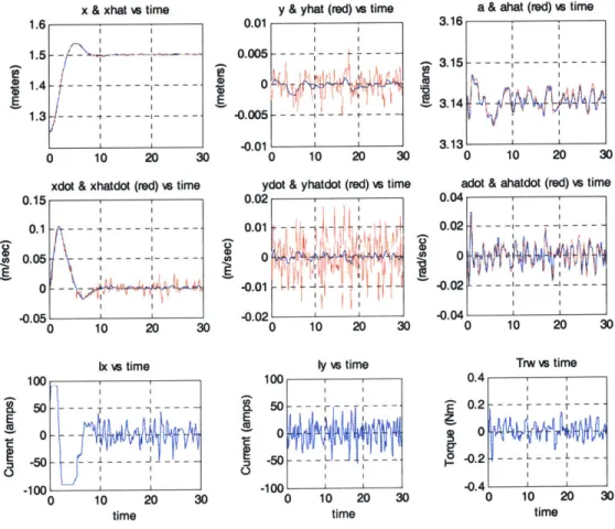
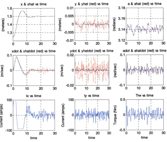
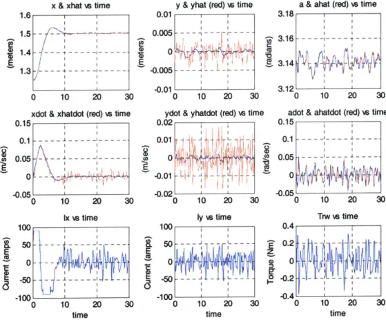
5.5.1 Radial Step Response... 85
5.5.2 Shear Step R esponse...89
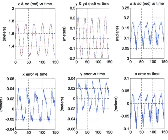
5.5.3 Radial Trajecto y ... 94
5.5.4 Shear Trajectory...97
CHAPTER 6: EXPERIMENTAL RESULTS.. ... 101
6.1 ORIGINAL CONTROLLER STEP RESPONSE ... 101
6.1.1 R esults ... ... 102
6.1.2 Comparison w ith Sim ulation...105
6.2 M ODIFIED CONTROLLER ... 107
6.3 MODEL FITTING ... 111
6.4 COMPARISON OF EXPERIMENTAL RESULTS WITH MODIFIED SIMULATION... 115
CHAPTER 7: CONCLUSIONS... . ... ... 127
7.1 T HESIS SUM M ARY ... ... ... 127
7.2 C ONCLUSION S...129
7.2.1 Success of Thermal Design...129
7.2.2 Comparison of Control Models... ... 129
7.3 RECOMMENDATIONS... ... 130
APPENDIX A ... ... ... 133
APPENDIX B ... ... ... 135
LIST OF FIGURES
FIGURE 1.1: FORCES AND TORQUES BETWEEN TWO DIPOLES... 16
FIGURE 2.1: ORIGINAL COIL SIZE ... 23
FIGURE 2.2: M ILLED FOAM CONTAINER ... 23
FIGURE 2.3: ORIGINAL LN2 TANK ... 24
FIGURE 2.4: ORIGINAL EM FF VEHICLE ... 25
FIGURE 2.5 AVIONICS DATA-FLOW DIAGRAM ... 26
FIGURE 2.6: DYNAMIC SIMULATION, 10% INITIAL CONDITION ON AR: STATE RESPONSES...29
FIGURE 2.7: DYNAMIC SIMULATION, 10% INITIAL CONDITION ON AR: ACTUATOR SIGNALS ... 30
FIGURE 2.8: LINEAR AIRTRACK ... 31
FIGURE 2.9: OPEN- AND CLOSED-LOOP STEP RESPONSES OF STABLE AIRTRACK ... 32
FIGURE 2.10: OPEN- AND CLOSED-LOOP RESPONSES OF UNSTABLE AIRTRACK ... 33
FIGURE 2.11: ANGLE-TRACKING RESULTS USING ONE VEHICLE ON THE PLANAR TESTBED ... 34
FIGURE 3.1: COPPER TEST PIECES...36
FIGURE 3.2: SOLDER HEAT TEST...37
FIGURE 3.3: NEW CONTAINER DESIGN...37
FIGURE 3.4: CONTAINER D IMENSIONS ... 38
FIGURE 3.5: NEW COIL DIMENSIONS...38
FIGURE 3.6: FIBERGLASS SPACERS...39
FIGURE 3.7: W IRE CONNECTION PORT ... 40
FIGURE 3.8: CONTAINER M OUNTS ... 40
FIGURE 3.9: PRESSURE REGULATOR CONCEPT...42
FIGURE 3.10: PRESSURE REGULATOR TEST W ITH W ATER...43
FIGURE 3.11: PRESSURE REGULATOR TEST WITH LIQUID NITROGEN... 45
FIGURE 3.12: TANK PLACEMENT ASSUMPTIONS...47
FIGURE 3.13: TANK PLACEMENT OPTIMIZATION ... 47
FIGURE 3.14: TANK CONNECTION PIPES ... 48
FIGURE 3.15: PRESSURE REGULATOR W EIGHT ... 49
FIGURE 3.16: INITIAL EM FF REDESIGN ... 49
FIGURE 3.17: SUPERCONDUCTOR BURN...50
FIGURE 3.18: SUPERCONDUCTOR BURN FIXES... 51
FIGURE 3.19: PRESSURE REGULATOR Fix ... 51
FIGURE 4.1: EM FF DATA FLOW DIAGRAM ... 53
FIGURE 4.2: DSP PROCESSOR ... 54
FIGURE 4.4: M ETROLOGY PROCEDURE ... 56
FIGURE 4.5: M ETROLOGY HARDWARE...56
FIGURE 4.6: G YROSCOPE...57
FIGURE 4.7: REACTION W HEEL TACHOMETER SENSORS...57
FIGURE 4.8: RESISTANCE TEMPERATURE DETECTOR, FIGURE 4.9: CURRENT AND TEMPERATURE DISPLAY.58 FIGURE 4.10: ELECTROMAGNETIC COIL BEHAVIOR ... 59
FIGURE 4.11: REACTION W HEEL DIMENSIONS ... 59
FIGURE 4.12: REACTION W HEEL STEP RESPONSE ... 60
FIGURE 4.13: FRICTION TERM OF REACTION WHEEL MODEL VS. SPEED ... ,...,,61
FIGURE 5.1: TESTBED SET-UP ... ,,,,. .,,,,63
FIGURE 5.2: MAGNETIC DIPOLE APPROXIMATION OF COIL OF CURRENT...65
FIGURE 5.3: TESTBED SET-UP WITH FAR-FIELD APPROXIMATION ... 65
FIGURE 5.4: COIL SET-UP FOR NEAR FIELD INTEGRATION...67
FIGURE 5.5: THE SLIDING CONDITION ... 77
FIGURE 5.6: SATURATION FUNCTION, SAT(S/ ( ) ... 78
FIGURE 5.7: TESTBED CONTROL SIMULATION ... 81
FIGURE 5.8: LINEAR FAR-FIELD CONTROLLER SINUSOID TRAJECTORY FOR CONTROLLER DEVELOPMENT... 83
FIGURE 5.9: NONLINEAR CONTROLLER SINUSOID TRAJECTORY FOR CONTROLLER DEVELOPMENT...,84
FIGURE 5.10: STEP RESPONSE IN X, FAR-FIELD CONTROLLER, FAR-FIELD MODEL ... 85
FIGURE 5.11: STEP RESPONSE IN X, FAR-FIELD CONTROLLER, NEAR-FIELD MODEL...86
FIGURE 5.12: STEP RESPONSE IN X, NEAR-FIELD CONTROLLER, NEAR-FIELD MODEL ... 87
FIGURE 5.13: STEP RESPONSE IN X, NONLINEAR CONTROLLER, FAR-FIELD MODEL...88
FIGURE 5.14: STEP RESPONSE IN X, NONLINEAR CONTROLLER, NEAR-FIELD MODEL ... 89
FIGURE 5.15: STEP RESPONSE IN Y, FAR-FIELD CONTROLLER, FAR-FIELD MODEL ... 90
FIGURE 5.16: STEP RESPONSE IN Y, FAR-FIELD CONTROLLER, NEAR-FIELD MODEL...91
FIGURE 5.17: STEP RESPONSE IN Y, NEAR-FIELD CONTROLLER, NEAR-FIELD MODEL ... 92
FIGURE 5.18: STEP RESPONSE IN Y, NONLINEAR CONTROLLER, FAR-FIELD MODEL...93
FIGURE 5.19: STEP RESPONSE IN Y, NONLINEAR CONTROLLER, NEAR-FIELD MODEL ... 94
FIGURE 5.20: LINEAR CONTROLLER, NEAR-FIELD MODEL SINUSOID IN X ... 95
FIGURE 5.21: NONLINEAR CONTROLLER, NEAR-FIELD MODEL, SINUSOID IN X ... 95
FIGURE 5.22: LINEAR CONTROLLER, SINUSOID IN X ERROR ... 96
FIGURE 5.23: NONLINEAR CONTROLLER, SINUSOID IN X ERROR ... 97
FIGURE 5.24: LINEAR CONTROLLER, NEAR-FIELD MODEL, SINUSOID IN Y ... 98
FIGURE 5.25: NONLINEAR CONTROLLER, NEAR-FIELD MODEL, SINUSOID IN Y ... 98
FIGURE 5.26: LINEAR CONTROLLER, SINUSOID IN Y ERROR ... 99
FIGURE 5.27: NONLINEAR CONTROLLER, SINUSOID IN Y ERROR ... 100
FIGURE 6.2: STEP RESPONSE IN X, CHEAP CONTROL... 103
FIGURE 6.3: X-POSITION STEP RESPONSE IN X, EXPENSIVE CONTROL ... 104
FIGURE 6.4: STEP RESPONSE IN X, EXPENSIVE CONTROL ... 105
FIGURE 6.5: STEP RESPONSE IN X, CHEAP CONTROL, SIMULATION AND EXPERIMENTAL RESULTS ... 106
FIGURE 6.6: STEP RESPONSE IN X, EXPENSIVE CONTROL, SIMULATION AND EXPERIMENTAL RESULTS...107
FIGURE 6.7: STEP RESPONSE IN X, CHEAP CONTROL MODIFIED...109
FIGURE 6.8: X POSITION STEP RESPONSE IN X, EXPENSIVE CONTROL MODIFIED... 110
FIGURE 6.9: STEP RESPONSE IN X, EXPENSIVE CONTROL MODIFIED... 111
FIGURE 6.10: MODEL FITTED TO STEP RESPONSE IN X USING CHEAP CONTROL MODIFIED ... 114
FIGURE 6.11: STEP RESPONSE IN X, CHEAP CONTROL ORIGINAL, MODIFIED SIMULATION ... 116
FIGURE 6.12: STEP RESPONSE IN X, CHEAP CONTROL ORIGINAL, MODIFIED SIM WITH TABLE SLOPE... 117
FIGURE 6.13: STEP RESPONSE IN X, EXPENSIVE CONTROL ORIGINAL, MODIFIED SIMULATION ... 118
FIGURE 6.14: STEP RESPONSE IN X, EXPENSIVE CONTROL ORIGINAL, MODIFIED SIM WITH TABLE SLOPE.. 119
FIGURE 6.15: STEP RESPONSE IN X, CHEAP CONTROL MODIFIED, MODIFIED SIMULATION...120
FIGURE 6.16: STEP RESPONSE IN X, CHEAP CONTROL MODIFIED, MODIFIED SIM WITH INITIAL COND...121
FIGURE 6.17: STEP RESPONSE IN X, EXPENSIVE CONTROL MODIFIED, MODIFIED SIMULATION...122
FIGURE 6.18: STEP RESPONSE IN X, EXPENSIVE CONTROL MODIFIED, MODIFIED SIM WITH TABLE SLOPE .123 FIGURE 6.19: ATTRACTIVE STEP RESPONSE IN X, EXPENSIVE CONTROL MODIFIED, MODIFIED SIM...124
FIGURE 6.20: ATTRACTIVE STEP RESPONSE IN X, EXP. CONTROL MOD, MOD SIM WITH TABLE SLOPE...125
FIGURE A. 1: X POSITION IMPULSE RESPONSE IN X, EXPENSIVE CONTROL MODIFIED ... 133
FIGURE A.2: IMPULSE RESPONSE IN X, EXPENSIVE CONTROL MODIFIED ... 133
FIGURE A.3: Y POSITION IMPULSE RESPONSE IN Y, EXPENSIVE CONTROL MODIFIED ... 134
FIGURE A.4: IMPULSE RESPONSE IN Y, EXPENSIVE CONTROL MODIFIED ... 134
FIGURE B.5: MODEL FITTED TO STEP RESPONSE IN X USING CHEAP CONTROL ORIGINAL ... 135
FIGURE B.6: MODIFIED MODEL FITTED TO STEP RESPONSE IN X USING CHEAP CONTROL ORIGINAL...136
FIGURE B.7: MODEL FrITED TO STEP RESPONSE IN X USING EXPENSIVE CONTROL ORIGINAL ... 137
FIGURE B.8: MODIFIED MODEL FrrTED TO STEP RESPONSE IN X USING EXPENSIVE CONTROL ORIGINAL ... 138
LIST OF TABLES
TABLE 3.1: WATER TEST RESULTS ... 44
TABLE 3.2: EXPERIMENTAL RESULTS WITH LIQUID NITROGEN ... 45
TABLE 4.1: PROCESSOR DETAILS...54
TABLE 4.2: EMFF MASS AND INERTIA ESTIMATES... 62
Chapter 1
Introduction
1.1 Motivation
Electromagnetic Formation Flight (EMFF) provides an attractive alternative to traditional satellite systems. It takes advantage of the fact that formation flight requires precision control with respect to the other spacecraft in the formation, but not of the formation as a
whole. This technology provides potential for significant fuel savings, longer mission life, and increased versatility in spacecraft control. This thesis describes the Space System Laboratory's (SSL) efforts to prove the concept of EMFF in a two-dimensional environment.
1.1.1 Motivation for Formation Flight
Multiple spacecraft flown in formation provide many significant advantages to traditional, large satellites for many space missions. A formation of small space vehicles can gather more and better data than one spacecraft in orbit.' Multiple spacecraft can be used for space-based interferometery without the size constraints imposed by physical structures. This freedom allows for the creation of large sensor apertures for increased angular resolution. Small spacecraft also provide cost savings in manufacturing, packaging and launching. A mission executed by many small spacecraft can be easily upgraded or repaired by replacing the necessary spacecraft instead of replacing the whole system. There is also opportunity for modular design in formation flight that could lead to more effective and less expensive missions.
The space community is actively researching the topic of spacecraft formation flight. The Air Force Research Laboratory and NASA are both considering many Earth and space science missions using formation flight. One example of such a mission is the Terrestrial Planet Finder (TPF), which aims to discover Earth-like planets around Sun-like stars. One proposed architecture for TPF is an infrared interferometer made up of formation flown spacecraft.2
The Space Systems Laboratory at MIT has developed a formation flight testbed called SPHERES. This system is used to conduct ground testing with soccer-ball sized vehicles in two dimensions and has successfully demonstrated formation flight maneuvers including tracking and docking. Tests have also been conducted in a zero-gravity environment on NASA's KC-135 aircraft and will be conducted on the International Space Station in the near future.3
1.1.2 Motivation for Electromagnetic Actuation
Although formations of spacecraft have many advantages, one challenge is maintaining precise control over each element in the array. Many optical applications require controlling individual vehicle positions with very small error. Using traditional thrusters, this level of precision could use large amounts of fuel as mission life increases. Since formations of spacecraft rely on relative positions of their elements, savings could be made by using interaction forces between the vehicles. One option is to use electrostatic forces. By building up charge on the various vehicles, attraction and repulsion forces can be created. However, a more attractive alternative is to use magnetic forces. Two magnetic dipoles are able to produce shear forces in addition to attraction and repulsion forces. This phenomenon is depicted below, in Figure 1.1.
S
A,
BA B
Electromagnets provide the ability to vary the strength of the magnetic field and introduce a control input. The magnetic interaction of electromagnets made by coils of wire with current flowing through them can be approximated, at large distances as compared to their size, as the interaction of magnetic dipoles through their centers. Multiple magnetic dipoles through one point add to give a new resultant dipole. With three orthogonal coils of wire each, the effective dipole through the center of the vehicle can be steered, and two vehicles can move to any position with appropriate control. However, when magnetic dipoles are not aligned they introduce torques on each other. These torques can be counteracted by reaction wheels. With the addition of three orthogonal reaction wheels, all relative degrees of freedom can be controlled. The limitation of electromagnetic control is that it can only control relative position of the spacecraft in an array and cannot control the position of the center of mass of the formation.
The largest advantage of electromagnetic control over propellant-based thruster control is that it does not rely on a consumable resource. Electromagnetic forces can be produced with the correct use of electric current, which can be harvested from the sun's energy using solar panels. This allows the spacecraft's lifetime to be limited by its hardware life instead of by the amount of fuel on board. Another disadvantage of control with thrusters is that propellant can cause damage. Many optical experiments can be degraded by propellant contaminating sensitive instruments or by thruster plumes obstructing the view of the spacecraft. Docking procedures are also safer without the possibility of firing a thruster at another spacecraft.
The use of electromagnetism to introduce significant forces that are able to control spacecraft is enabled by superconducting technology. Conventional wire is not able to carry the current necessary to produce magnetic moments capable of controlling spacecraft motion to a reasonable level. However, high temperature superconducting
(HTS) wire has been developed that is capable of carrying 140 times the current of
copper wires of the same size. HTS wire must be cooled to temperatures below 115K to be superconductive.4 In this state the wire has zero resistance, which increases the
efficiency of this method. The challenge in implementing superconducting electromagnetism is cooling the wire coils to superconducting levels. Immersion in liquid nitrogen is effective in accomplishing this task and further investigation is being conducted into other methods of regulating cryogenic wire temperatures.
1.2 Testbed Description
A testbed has been developed at the MIT Space Systems Lab (SSL) to investigate the
feasibility of the Electromagnetic Formation Flight (EMFF) concept. Two vehicles have been built to test control algorithms using electromagnetic forces. Tests are conducted on a flat surface using pressurized CO2 to float the vehicles, simulating a frictionless
environment in two dimensions and giving each vehicle three degrees of freedom. The vehicles each have two orthogonal coils of superconducting wire and a vertical axis reaction wheel to provide full control authority. A liquid nitrogen containment system maintains a superconducting temperature for the wire. An infrared and ultra-sound metrology system provides position measurements and computation is executed by a
C6701 processor.
1.3 Thesis Overview
This thesis will describe the work done to implement reliable thermal and dynamic control of an Electromagnetic Formation Flight testbed. The next chapter will focus on the previous work done to develop EMFF. First we will look at the original design for thermal control that was pursued by a class at MIT. We will review the requirements used to come to this initial design, describe the architecture of the system, and investigate problems encountered. We will also give a description of the initial avionics design and reasons for its upgrade. We will next discuss the dynamic modeling and control work of Dr. Laila Elias. Finally, we will see results of implementing control both in simulation and using hardware experiments.
The third chapter will outline the new design for thermal control. First, we will describe the process of selecting materials for the system. Next, we will take a detailed look at the design of the thermal system. A simple, but innovative approach to pressure regulation
that is used for thermal control will also be explained. We will also look at problems that were encountered in the re-design of the thermal system and how they were fixed.
The fourth chapter will describe the EMFF system and its subsystems. These systems include the avionics, which handles all information and is used to program control algorithms, the metrology system, which uses information from multiple sensors to find the state of the vehicle at all times, and the actuators, which provide the forces and torques to manipulate the vehicles. The physical properties of the vehicle, which are used to develop control for the system, will also be identified.
In the fifth chapter we will describe the magnetic field models used to simulate the vehicle's dynamics and develop proper control. Next, various methods of control that are relevant to the EMFF system will be explained and the simulation developed to evaluate these controllers will presented. We will also look at the simulations behavior in rejecting disturbances and following trajectories.
The control algorithms developed in Chapter 5 were implemented on the EMIFF testbed to prove the ability to control an actual vehicle using electromagnetic forces. The results from these tests will be presented and compared to the predicted results from the simulation. A method will be introduced that was used to match the simulation model with what was observed in tests. A new model will be presented and its simulation predictions will be compared to the experimental results. Finally, we will conclude the thesis with a summary and highlight the contributions of this research.
Chapter 2
Previous Work
2.1 Thermal Control
Superconducting wire is an enabling technology for the EMFF concept. Conventional copper wire cannot carry the required current to create magnetic fields capable of controlling a formation of satellites and would put far too great a demand on the power subsystem to make it advantageous. However, along with this technology comes the challenge of keeping the wire at temperatures needed to enable superconducting. This section describes the design pursued by the MIT Department of Aeronautics and Astronautics Junior/Senior Capstone Design Class (CDIO) to provide this thermal control.
2.1.1 Requirements
The superconducting wire, purchased from American Superconductor, must be kept below 115K to exhibit superconductive characteristics. Below this temperature, the wire has zero resistance, but as temperature drops the amount of current that can be carried by the wire increases.4 If a cryogenic fluid is used to provide cooling of the coils, the wire
must be completely submerged by that fluid. The cooling fluid must also be insulated from the environment, which is at a much higher temperature. The containment system for the superconducting coils must fulfill these requirements.
The class also set specifications for what kind of maneuvers the system should be able to execute. To show its potential for use with interferometers, a formation of two EMFF vehicles must be able to spin-up to a rate of one rotation per minute. This requirement
directly feeds the sizing of the superconducting coils because they must be large enough to provide a magnetic moment capable of accelerating the formation to the required rate.
A final requirement of the thermal control for EMFF is that it be completely
self-contained on each vehicle. It must be structurally connected to the rest of the vehicle and not require connection to any other components while testing. Although the thermal control system can be refilled between tests, the system must be designed to be completely autonomous during tests. Tests are to run for twenty minutes without the vehicles needing additional cooling fluid.
2.1.2 Previous Design Description
The CDIO class designed a superconducting wire and thermal control system to meet the requirements outlined for the EMFF system. A detailed description can be found in the design appendix created by the class.5 To provide the forces and torques necessary to spin-up a two-vehicle array to one rotation per minute, each electromagnet must provide a maximum magnetic moment of t = 4723 [A-m2]. Magnetic moment of a coil of
current-carrying wire is the product of the number of turns of wire, the amount of current, and the area enclosed by the coil, or g = nIA. The superconducting wire used can carry up to 100 amps without reaching its critical current, which leaves the number of turns and size of the coil to be chosen. The team decided on coils of diameter close to one meter.
The outside coil was designed to have a diameter of .835 meters and 99 turns of wire. The inside coil had a diameter of .670 meters and 120 turns of wire. Each superconducting coil was made up of three coils in series. This design allowed the entire coil cross-section to take a more geometrically efficient, square shape. Kapton insulation was applied between the turns of the wire to prevent any electric shorting across the wires. The dimensions of the coils are depicted in Figure 2.1.
Outer Coil
1.5 cm
Inner Coil
2.0 cm
Figure 2.1: Original Coil Sizes
The casing for the superconducting coils was made of STYROFOAM, extruded polystyrene insulation, milled in a toroidal shape. This casing provided the structure to hold the coils and liquid nitrogen as well as the insulation to isolate it from the environment. Spacers were cut into the foam to hold the superconducting wire and allow room for liquid nitrogen to pass freely. The containment system was made so the entire smaller container fit inside the larger one (Figure 2.4). The foam pieces were attached to each other using epoxy, and fiberglass tape was wrapped around the containers and sealed with epoxy to provide leak-proofing.
Figure 2.2: Milled Foam Container5
To provide a sufficient test duration, a tank was designed to supply the system with liquid nitrogen as it boiled off. A simple gravity-fed system was implemented. The 12-inch square tank was installed above the two coils so that the liquid nitrogen would fall into the containers to keep the coils submerged and at cryogenic temperatures. The tank was designed to provide 10 minutes of cooling.
Figure 2.3: Original LN2 Tank5
2.1.3 Problems with Initial Design
Thermal cycling from repeated cooling to cryogenic temperatures and returning to room temperature created cracks in the foam containment system. Fiberglass tape and epoxy were used to seal these leaks. It was thought that after multiple thermal cycles, the stress in the foam would be relieved and no additional cracks would form. However, with nearly every filling of the containment system, new leaks would form. After most tests, the leaks would need to be marked and then the vehicle would have to warm to room temperature and dry out completely. The next day fiberglass tape and epoxy would be wrapped around the leaking area and the vehicle would be ready for tests in the next couple days. Several successful tests were conducted under these circumstances, but the constant leaks were disruptive to the test schedule. Frequent re-patching also added weight to the vehicle.
The LN2 tank placement also presented problems. Filling the containment system was difficult since the top of the tank was not visible or reachable from ground level. Pipes were used to pump the liquid nitrogen to the top of the vehicles and into the tank. The tank also made the EMFF vehicle top-heavy and added unnecessary height to the vehicle. The containment system also lacked secure mounts to the vehicle base permitting the coils to lean to the side.
Figure 2.4: Original EMFF Vehicle
2.2
Avionics
The CDIO class also identified the interfaces of the avionics/electronics subsystem needed for the EMFF vehicle. "The primary role of the avionics subsystem is to integrate all hardware and software of the system".5 The core of the initial avionics was the Tattletale Model 8 computer. The Tattletale Model 8 computer (TT8), with Motorola
CPU (Central Processing Unit) and TPU (Time Processing Unit) was chosen because it
was thought to suit the project processing needs and it was readily available in the Space Systems Laboratory. The computer interfaced directly with four other pieces of
hardware: The Metrology computer, the voltage regulator, the Communications board, and a series of mosfets used for power amplification purposes. This hardware conceptual layout is shown below, in Figure 2.5.
-. 232
i L
-U
Figure 2.5 Avionics Data-flow Diagram5
The Metrology computer was an additional Tattletale Model 8 computer. The avionics subsystem was designed to allow the sending of the vehicle's state information using Primary Vehicle Array (PVA) updates through a serial channel from the Metrology TT8 to the main Avionics TT8 computer. The power subsystem was designed to supply steady 5V power from the AA batteries to the Tattletale computers and the Avionics board. The communications/operations hardware was designed to send and receive all data being transmitted and received from the immediate vehicle system to the avionics
TT8 and vice versa. The communications board interfaced with the avionics TT8
through a serial RS232 cable connection.
Although the initial avionics design allowed for functionality of the testbed, there were limitations that were found. Since the electronics were integrated by hand, some connections were not reliable and signals were occasionally corrupted, resulting in bad
data. The integration of wireless communications was also found to be quite difficult and would have required extensive work to complete. Successful tests were completed using tethers between the vehicles and ground station for communications, but the tethers introduced external forces that disturbed the dynamics of the system. Finally, there was not enough computational speed in the TT8 to perform complex control algorithms.
2.3 Dynamics and Control
Previous work has been completed to model the dynamics of the EMFF system. Dr. Laila Elias conducted research in the Space Systems Lab to develop a full 3-dimensional model of EMFF using dipole approximations for the interactions between electromagnets. She also analyzed the stability and controllability of such a system, as well as performing relevant experiments to improve confidence in the technology of EMFF.6
2.3.1 Three-Dimensional Dynamics Model
The interaction forces and torques between current carrying coils of wire can be approximated by treating the coil as a magnetic dipole through the coil center along its axis. This approximation is valid at separation distances much larger than the coil's radius. The dipole has an effective magnetic moment equal to the product of the number of turns of wire, the amount of current, and the area enclosed by the coil, or p = nIA. The forces and torques created from the interaction of magnetic dipoles depend nonlinearly on their positions. Other nonlinear dynamics occur in the EMFF system due to the effects of gyroscopic stiffening from spinning reaction wheels. These inherent nonlinearities require a nonlinear model to describe the dynamics.
Nonlinear equations of motion were developed for a multi-spacecraft array using EMFF technology. The geometry of such an array was defined with multiple coordinate systems and a standardized notation was introduced. The dynamic model included the nonlinear dynamics of the reaction wheels and also accounted for external disturbances to the system. The general form of these equations is valuable because it can be adapted to describe any more specific situation. By eliminating degrees of freedom and only using
two vehicles, the dynamic model can be changed to describe the two-dimensional testbed that is functioning in the lab.
In Elias' thesis, the general dynamic model was then simplified to two vehicles. The system dynamics were linearized about a nominal trajectory, a steady-state spin. This trajectory is significant because it is a maneuver needed by interferometer configurations. In a steady-state spin, the spacecraft need a constant attractive force to counter the centrifugal accelerations pulling them apart. Additional control is needed to reject disturbances and remain on the nominal trajectory.
The linearized dynamics of the nominal trajectory were then analyzed for stability. They were found to be unstable with a pole in the right half plane. It was found that instability grew with increased nominal spin rate. However, controllability analysis shows that the system is stabilizable. It was shown that an EMFF system with three orthogonal coils and three reaction wheels is fully controllable in three dimensions. A two dimensional system is also fully controllable with two orthogonal coils and one reaction wheel. This validates the design of the two dimensional EMFF testbed.
An optimal controller was then designed to stabilize the linearized dynamics of the nominal trajectory. A linear quadratic regulator was developed to minimize a weighted sum of state errors and control use. A large part of this work was in determining appropriate penalties for state errors and actuator use.
The optimal controller was used in a closed-loop simulation to evaluate its effectiveness. This simulation used the nonlinear equations of motion describing the system to model its
behavior. State feedback from this model was used by the LQR controller to calculate the appropriate control to apply to the nonlinear model, completing the control loop. The simulations used various Matlab differential equation solvers.
Closed-loop control simulations tested the system's ability to arrive at the nominal trajectory after starting at off-nominal initial conditions. Analyzing the behavior of the
free response to these non-zero conditions gives similar information as investigating the system's response to disturbances. The results of these simulations showed that the
EMFF system is indeed stabilizable. The controller was able to bring the behavior of the
system to its nominal trajectory with feasible magnitudes of control. The simulations also showed that a limiting factor in controlling the EMFF system could be the torque capabilities of the reaction wheel motor.
UNEAR vs. NONLINEAR Sim Using Optimal Controf (10% IC on Ar)
1 - - - ---- ---- -- -- - - -- - -.-.--. UnerSim 0 ~ -Nonlinar Sim . ... .... .... ... .. l .. A O.. - A f . .. 7 W . 9 -0 0 ... Acv m ... an ... 0 ... 0 ... rm ... .wan .... ....7nn ... 90 0 ... ... 0 - - - -- - -0. -0. 0 ...n~ tm Mf ... .. . 0 . .. ... ... .. . - --1 - - i 0 .. .11111111. 1.11111.1711... 0 ~ O 7~f ... 0 0 -2r 'l4 X 2 0 ) ... .. ...7 M 7. .. ...... .. . .A Ml. .... .... .. . 719 IC ) . ... .1M~ ~ ~ ~ ?W ... ... ... A ... A ...I R 0 100 200 300 400 500 Trne [s] 000 700 800
Figure 2.6: Dynamic Simulation, 10% Initial Condition on Ar: State Responses6
±4
U
I-i
IUNEAR vs. NONLIUNEAR Sim Using Optnal Control (10% IC on Ar)
-2 -2 1 -,WMA' a- ... T -2 2 22 ... -2 TI1~ -F T T ... ... . ... . .. 2rr Mr
T
a
2 II I ... TTo
.4 .s
. . a@- . .... -ro -... saa -r-ro
... e1 O 00 M 300 40 500 "00 n00o
Tme [secl
Figure 2.7: Dynamic Simulation, 10% Initial Condition on Ar: Actuator Signals'
2.3.2
Hardware Experiments
Previous work has also been done in experimentally testing the feasibility of electromagnetic control. Elias' thesis describes experiments conducted in a one-dimensional environment using an airtrack as well as initial work on the two-one-dimensional
EMFF testbed. This work has provided positive results encouraging further investigation
into the effectiveness of this technology.
The linear airtrack consisted of an electromagnet fixed to one end of a track and a permanent magnet that was free to slide on the track. The current flowing through the electromagnet could be adjusted in real time to provide control authority. Compressed air was fed through small holes in the track to enable the permanent magnet to slide freely. An ultrasonic displacement sensor was used to determine the position of the sliding magnet in real time. This feedback information was used to develop controllers to
regulate the position of the free magnet. Experiments were conducted in both a stable and an unstable configuration.
Figure 2.8: Linear Airtrack6
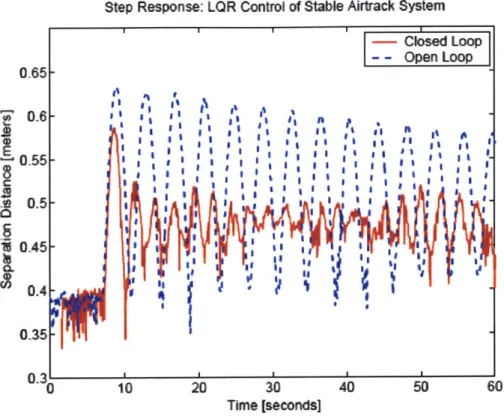
The air track was configured to be stable by slightly tilting the track so the free magnet tended to slide towards the electromagnet. Although stable, the step response of this system was highly oscillatory. By implementing a feedback controller, the behavior was significantly improved.
Step Response: LOR Control of Stable Airtrack System '.' O. 6 I I - r. It 0.4 J 010 20 30 40 50 60 Time [seconds]
Figure 2.9: Open- and Closed-Loop Step Responses of Stable Airtrack'
Experiments were also conducted with the track tilted so the sliding magnet fell away from the electromagnet. This unstable configuration of the air track is of more interest because its dynamics are very similar to those of a steady-state spin of a spacecraft array. In both situations a constant force is required to oppose the forces pulling the two magnets apart. If the force between them is slightly too large, the magnets will crash into each other and if it is slightly too small they will drift apart. For this reason, feedback control is needed to maintain constant separation distance. Experimental results showed that this unstable system can be controlled.
LQR Control of Unstable AirtracK System W0.8 -E0.67- -* I 0 -@ 0.5 a 0.4 0.3-g A~~ 02-010 20 30 40 50 60 Time [seconds]
Figure 2.10: Open- and Closed-Loop Responses of Unstable Airtrack'
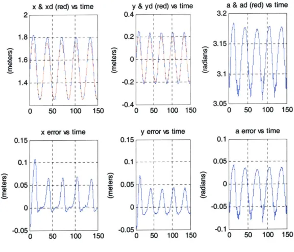
Successful results on the linear air track imply that the proposed control of two and three dimensional systems are also likely possible. At the time of Elias' thesis the two-dimensional EMFF testbed was not fully functional because the metrology system was not working. However, reaction wheel control was successfully implemented to regulate the attitude of the spacecraft. The results are shown below.
Test Case Ib: Tracking Angle Commands (October 2003)
0 10 20 30 40 50 60
Time [s]
Figure 2.11: Angle-Tracking Results Using One Vehicle on the Planar Testbed'
-Chapter 3
New Thermal Design
The problems faced with the original thermal design could not be permanently fixed with repair, so a new design was needed. The new thermal system needed to be leak-proof, lightweight, and professional in appearance. This section outlines the process of designing this new thermal control system for the EMFF testbed vehicles.
3.1 Material Selection
Styrofoam has many qualities that made it attractive as a material for the first containment system. It is easy to shape with a lathe or by carving with a knife. It is also a good insulator, which helps isolate the liquid nitrogen from the environment, and it is not magnetic. Foam is also very light-weight, yet strong enough to hold the wire coils. Unfortunately, it also cracks easily so it could not handle the thermal deformations caused by cryogenic temperatures.
Most of these characteristics were looked for in a new material. Plastic seemed like a good option, but it could not handle the thermal extremes induced by liquid nitrogen. Next, metals were investigated. Since the containment system is in the shape of a torus, the metal would need to be ductile. We chose to test copper because it is not magnetic, it can be soldered at its joints, and as a sheet it can be bent easily.
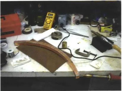
A system made of copper would depend on strong, leak-proof solder joints. A test piece
of copper soldered into a ring was procured and inspected for strength. It was thermally cycled from room temperature to liquid nitrogen temperatures multiple times. The joint
showed no sign of cracking and maintained its strength. A box channel made of thin copper sheet was made to test for rigidity and strength. It was found that in a box formation, very thin copper could be used to make a strong structure.
Figure 3.1: Copper Test Pieces
Another requirement of the containment system is imposed by the superconducting wire. The wire can delaminate at temperatures above 3000 F and be destroyed. When installing the superconducting coil, the containment system would have to be soldered closed at high temperatures. A test was set up to determine the internal temperature of a channel as a lid was soldered onto it. Temperature readings were recorded throughout the soldering process, both with and without air flowing through the channel. Tests were conducted using both a torch to solder and a soldering iron. The soldering iron kept the internal temperatures lower and was easier to use. Tests using a soldering iron reached a maximum temperature of 1100 F with airflow cooling, and 1800 F without. These results show that a soldering iron can be used to heat the copper container without damaging the superconductor inside.
Figure 3.2: Solder Heat Test
3.2 Design Description
A toroid shaped container was designed for the EMFF vehicles using copper. The
containers were designed to provide " of space between the walls and the coil to allow the liquid nitrogen to pass freely around the coil. The container was designed as a rectangular channel with a flange at the top as shown below. The lid is flat and can be placed on top and soldered to seal the container.
Lid
Solder
The large coil set the size for the first container. It was designed to fit the three coils of superconductor inside with approximately " of space around each coil. The superconducting wire is 0.24 inches wide. The large container holds three coils of wire each with a diameter of 32.87 inches and 99 turns. Since the copper containers are much smaller than the previous foam containers, the inner coil was re-wrapped to a larger diameter. It now is 30.62 inches in diameter and each coil has 103 turns. The container designs are shown below. The lid is the same size and shape as the container, but only a single sheet of copper.
I III
Figure 3.4: Container Dimensions
Outer Coil
0.55 iJ
I
Inner Coil
I I
Figure 3.5: New Coil Dimensions
The coil is held away from the wall of the container with spacers made of fiberglass. The spacers are cut by a water jet so the coil of wire fits into them snuggly. The fiberglass provides electrical insulation between the wires and the container, as well as thermal insulation from the copper walls. The spacers are attached to the coil on alternating sides with additional spacers at the bottom and top of the container.
~mm~m~j;
Figure 3.6: Fiberglass Spacers
To keep the container leak-proof, a special electrical connection had to be designed for passing current to the coils. The containers were designed with protruding connection ports to make room for attaching the superconducting wire to the connector. A 3/16 inch diameter copper rod is used to pass current through the container. Teflon shrink tubing surrounds the copper rod to provide electrical insulation from the container. The connector uses a pipe compression fitting to create a leak-tight seal around the conductor.
Figure 3.7: Wire Connection Port
An advantage of using copper for the containment system is that connecting pieces can be easily soldered onto the container. Tabs were soldered to the top and bottom of each container for alignment. The bottom tabs were fastened to a mount on the vehicle base. The mounts are made of fiberglass screwed into aluminum blocks. They provide a secure, rigid connection for the container.
Figure 3.8: Container Mounts
Reflective aluminum foil insulation was chosen to wrap around the containment system and provide a barrier between the warm air of the laboratory and the cryogenic temperatures of the containment system. The insulation is constructed of two layers of thin aluminum sheet separated by a 5/16 inch dead air space. This type of insulation was chosen because it can be easily wrapped around the containment system without greatly increasing the size of the vehicle.
3.3 Pressurized System
In order to make the vehicles less top-heavy and more compact, it was decided to put the liquid nitrogen tank inside the coils. Placing the tank below the top of the containers necessitates a pressurized cooling system. One option would be to constantly pump liquid nitrogen through the containers. This would require an expensive and heavy cryogenic pump. Instead, a simple concept, resembling a pressure cooker, was investigated.
3.3.1 Concept Evaluation
To fill the containers with liquid nitrogen there must be enough pressure in the tank to lift the liquid nitrogen to the top of the containers. A constant pressure will cause a constant height difference between the liquid surfaces in the tank and in the containers. The difference in pressure at the two surfaces determines the vertical distance between them, which depends on the density of the fluid.
AP= pgh (3.1)
As liquid nitrogen sits in the tank it evaporates slowly. As it changes from liquid to gas it expands to 694 times its volume. This expansion creates a high pressure inside the tank. To maintain a constant pressure, a valve is needed that releases excess gas when the internal pressure is higher than desired. Pressure is a ratio of force to area, so by creating a pressure regulator with a weight sitting on a hole with the correct weight to area ratio, the desired pressure can be regulated. When the pressure inside the tank reaches the ratio
of the weight to the area of the opening, the weight will lift and allow gas to escape until the pressure falls to the desired level. This concept is illustrated below.
h=AP/(pg)
FF
Hole with AP=F/A
area, A
Figure 3.9: Pressure Regulator Concept
A simple version of this kind of valve is a ball sitting on a hole in the tank. The pressure
will build in the tank until it reaches the ratio of the ball's weight to the area of the hole. Then the ball will lift and release pressure until the ball can fall back onto the hole. An experiment was set up to test this concept. A clear tube was connected to the bottom of a tank and then hung vertically next to it. The tank was filled with water and the level in the tank was the same as the level in the clear tube. A metal ball was placed on top of a fitting in the top of the tank and pressurized air was fed into the top of the tank. After the pressure built up inside the tank, the ball lifted and floated on the escaping air. The water level in the tube was recorded. This procedure was repeated for balls of various masses.
Figure 3.10: Pressure Regulator Test with Water
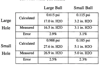
Two metal balls were used for testing, one weighing 1.6 ounces and the other 0.3 ounces. Two fittings, of different diameters, were used for the experiments. The larger fitting had a diameter of 0.455 inches and an area of 0.1626 in2. The opening on the smaller fitting was 0.359 inches across with an area of 0.1012 in2. Shown below are the pressures that were expected to be regulated by placing the ball on the fitting and pressurizing the tank. The pressures are shown in both pounds per square inch (psi) and in the height in inches that they should lift a column of water. The tests gave results very close to the calculated values. The maximum error was three percent. This showed that the proposed method of pressure regulation was promising.
Table 3.1: Water Test Results Large Ball Large Hole Small Hole Small Ball 0.615 psi 0.115 psi Calculated 17.0 in. H20 3.2 in. H20
Measured 16.5 in. H20 3.1 in. H20
Error 2.9% 3.1% 0.988 psi 0.185 psi
Calculated
27.6 in. H20 5.1 in. H20
Measured 26.9 in. H20 5.0 in. H20
Error 2.5% 2.3%
This experimental setup was adapted to allow for testing with liquid nitrogen. Instead of a plastic tube, a large copper pipe was attached to the bottom of the tank. A Styrofoam float with a wooden rod was used to check the level of liquid nitrogen in the pipe. The same experiment that was done with water was not as successful with liquid nitrogen. When a ball was placed on a fitting the level of LN2 would quickly rise to a level slightly higher than what was expected. Then the level would slowly increase much higher than expected. It was thought that the nitrogen gas could not escape quickly enough through the fitting, so a new regulator was built. A weight was designed to slide freely in a large pipe, but to completely cover a hole of slightly smaller diameter. A plug with a hole of this diameter was soldered into a pipe to create the regulator shown below. The larger hole allowed gas to escape more freely and allowed better pressure regulation.
Level
Indicator
Pressure Regulator
Figure 3.11: Pressure Regulator Test with Liquid Nitrogen
Small rings were added to the weight shown above to investigate the liquid level response to increasing weight. The initial weight was 2.3 oz and each ring added 0.2 ounces. The tests showed that the level of liquid nitrogen could be controlled reliably to within 5% error using a regulator similar to the one used in our experiment.
Table 3.2: Experimental Results with Liquid Nitrogen
Weight Calculated Actual Average
% Error
2.3 oz 2.5 oz 2.7 oz
25.0 in. LN2 27.3 in. LN2 29.4 in. LN2
24.2 in. LN2 26.0 in. LN2 29.3 in. LN2
3.2 4.8 0.34
3.3.2 Implementation
The first element in the pressure regulation system is the tank. The tank was designed to hold twice the amount of liquid required to fill the containment system. The volume of the tank was set at 550 in3. With appropriate insulation this should provide twenty minutes of cooling. It was also decided that the tank would be a cylinder because of the ease of manufacturing this shape. Using a constant volume, the size and placement of the tank were optimized, constrained by the size of the smaller container. The goal was to find the optimal geometry and placement of the tank between the extremes of a tall, narrow column in the center of the vehicle and a short, wide disc in the middle of the
vehicle.
Since electronics, the reaction wheel, and other components needed to fit in the middle of the vehicle, the tank was designed to sit as low as possible inside the containers. The tank width was constrained to fit inside the smaller ring, with margin for the insulation that would be applied. Below is the optimization that yielded the most efficient placement and size of the tank. As the position of the bottom of the tank is lowered (shown as an increasing d), the calculated location for the top of the tank also decreases to a point. After this point, the tank starts to look like a tall cylinder, which would take up most of the space inside the vehicle.
V =7b 2h b=4r 2-2 V h=-7tb2 H=h-d
Figure 3.12: Tank Placement Assumptions
Figure 3.13: Tank Placement Optimization
The top of the tank is lowest when the distance to the bottom of the tank from the center of the vehicle is 10.4 inches. This yields a tank that has a diameter of 15.56 inches and a height of 2.88 inches. This puts the bottom of the tank 28 inches below the top of the
large container. The pressure regulator must be designed to lift the liquid nitrogen level in the containers to at least 28 inches.
The tank was made by bending a strip of copper into a cylinder shape and soldering it to a circle of copper on the top and bottom. It was attached to the containers with pipes that connected to compression fittings. This allows the tank to be easily removed from the containers and maintains the system's modularity.
Figure 3.14: Tank Connection Pipes
The specific weight of liquid nitrogen, or density times gravitational acceleration, is
0.02919 lb/in3. Therefore 0.82 psi is needed to raise the liquid nitrogen level 28 inches.
A pressure regulator similar to the one used in proving the concept was designed. Its
opening has a diameter of 0.50 inches and an area of 0.20 in2. To regulate the desired pressure the weight needed to be 2.568 ounces. The weight was made of brass and designed to have a volume of 0.519 in3 to provide the necessary weight. A drawing of the weight is shown in Figure 3.15. Rings were also made to add weight if needed.
Figure 3.15: Pressure Regulator Weight
3.4 Design Evolution
The thermal control upgrade has shown improved performance over the original design. However, the design has evolved as problems were identified and fixed. Below is the first version of the new design. This section outlines the flaws discovered and the work done to resolve them.
Figure 3.16: Initial EMFF Redesign
3.4.1 Superconductor Burn
It was found that the placement of the connectors to the superconducting coils was not ideal. In two coils, the superconductor broke from apparent burning near the point of connection. It is thought that an air bubble formed around the superconductor next to the connector, allowing it to increase temperature, and causing it to cease superconducting. In review, it was seen that the geometry of the connection port could lend well to this phenomenon.
The point of the connection port was slightly higher than the vent for escaping nitrogen gas. It is likely that gas was caught in this area and caused the superconducting wire to heat up past superconducting temperatures. The wire is separated from the rest of the coil at this point so it does not have the thermal mass to keep it from heating up quickly. As the wire became highly resistive, large amounts of current were continued to be driven into it. Too much power was dissipated, P= I2R, and the wire burnt through.
Possible gas pocket
First area to heat
up-Figure 3.17: Superconductor Burn
To ensure that the area where the superconducting wire exits the container stayed completely covered in liquid nitrogen, the connection point was lowered. This required the wall of the container to be cut at a lower point, bent outwards and patched with additional copper. As another safeguard, a temperature sensor, called a resistance temperature detector (RTD), was installed in the liquid nitrogen vent in each vehicle.
When the liquid nitrogen level falls below the sensor, a light turns red and current is not applied to the superconductors.
New connection
RTD
Figure 3.18: Superconductor Burn Fixes
3.4.2 Oscillating Pressure Regulator
The weight used in the pressure regulator valve was able to regulate the liquid nitrogen level accurately, but exhibited an oscillating behavior. The liquid level in the containers would reach the vent pipes and then slowly rise until the pressure regulator would let out a sudden burst of nitrogen gas and the level would fall below the top of the container and return again. The holes in the weight did not allow the gas to escape quickly enough until the pressure rose enough to lift the weight significantly. The sides of the weight were milled out to allow gas to escape. The behavior with the modified weight was much smoother, with a constant release of nitrogen to maintain the correct pressure.
Original ' Modified
Chapter 4
System ID and Description
The EMFF system is driven by a computer that reads inputs from multiple sensors, processes metrology measurements, handles communications procedures, calculates control outputs, and sends commands to actuators. This section will describe the components of this system and the physical properties of an EMFF vehicle.
4.1 Electronics description
4.1.1 Computer
A Texas Instruments C6701 DSP runs the flight software at a rate of 167 MHz. Table 1.1
shows the key characteristics of the computer.
Table 4.1: Processor Details3
DSP No. 1 Speed Mhz 167 FLOPS (Peak) G 1 RAM MB 16 Cache kB 512 ROM - available kB 224 ComPorts No. 6 CommPort Rate Mbps 20 Power W 7 Figure 4.2: DSP Processor3
Analog sensors are sampled and digitized by an FPGA at 12-bit resolution. It has a speed of 25 MiHz. The computer reads inputs from infrared and ultrasound receivers for metrology. It also senses information about the system from the reaction wheel tachometer, a gyroscope, a temperature sensor, and a current sensor. The computer also handles communications outputs and inputs. It outputs commands to the actuators, which are the reaction wheel and electromagnetic coils. The computer also outputs commands to the metrology system to signal it to send IR and US pulses.
4.1.2 Communications
The communications subsystem uses a radio frequency channel to transmit data. An RFM DR2000 is used to provide 57.6 kbps of raw data, or an effective 18 kbps. We send packets of 32 bytes at a rate of 70 packets of useful data per second. The
communications structure is time-division multiple access so the vehicles and laptop take turns communicating while the others listen. The communications period is split into windows for each vehicle to transmit.
Figure 4.3: RFM DR20003
4.1.3 Power
Each EMFF vehicle is equipped with two sets of eight AA batteries to power the avionics. A voltage regulator maintains supplies of 5 volts and 12 volts. Most avionics chips use the five volt supply, and the twelve volt supply is used by a circuit that displays information about the coils. Each electromagnetic coil has 3 D-cell batteries to provide the current used to create the electromagnet. The reaction wheel uses a separate supply of 7 D-cell batteries.
4.1.4 Metrology
The relative positions of the vehicles are determined real-time with a metrology system that uses infrared and ultrasound pulses. The metrology loop is initialized with a command for an infrared pulse that is sent by the FPGA. The infrared pulse is transmitted and then immediately received by all vehicles to synchronize their timing. Next the vehicles take turns sending ultrasound pulses. The receiving vehicle knows when the transmitting vehicle sent its US pulse and counts the time until it receives the pulse. Since the speed of sound is known, this time count can be converted to a distance.