HAL Id: hal-02609736
https://hal.inrae.fr/hal-02609736
Submitted on 16 May 2020
HAL is a multi-disciplinary open access
archive for the deposit and dissemination of
sci-entific research documents, whether they are
pub-lished or not. The documents may come from
teaching and research institutions in France or
abroad, or from public or private research centers.
L’archive ouverte pluridisciplinaire HAL, est
destinée au dépôt et à la diffusion de documents
scientifiques de niveau recherche, publiés ou non,
émanant des établissements d’enseignement et de
recherche français ou étrangers, des laboratoires
publics ou privés.
Using Repeated Measures Experiments
A. Despax, Jérôme Le Coz, A. Hauet, D.S. Mueller, F.L. Engel, B. Blanquart,
Benjamin Renard, K.A. Oberg
To cite this version:
A. Despax, Jérôme Le Coz, A. Hauet, D.S. Mueller, F.L. Engel, et al.. Decomposition of
Uncer-tainty Sources in Acoustic Doppler Current Profiler Streamflow Measurements Using Repeated
Mea-sures Experiments. Water Resources Research, American Geophysical Union, 2019, 55, pp.7520-7540.
�10.1029/2019WR025296�. �hal-02609736�
Measurements Using Repeated
Measures Experiments
Aurélien Despax1 , Jérôme Le Coz1 , Alexandre Hauet2, David S Mueller4, Frank L Engel4 , Bertrand Blanquart3, Benjamin Renard1 , and Kevin A Oberg4
1Irstea, UR RiverLy, Lyon, France,2EDF-DTG, Grenoble, France,3Independent Expert, Nancy, France,4U.S. Geological
Survey, Reston, VA, USA
Abstract
Repeated measures experiments can be conducted to empirically estimate the uncertainty of a stream gauging method, such as the widespread moving-boat acoustic Doppler current profilers (ADCPs) approach. Previous ADCP repeated measures experiments, also known as interlaboratory comparisons, provided a credible range of uncertainty estimates reflecting the quality of the site conditions. However, the method, which is a one-way analysis of variance, only addresses the uncertainty of one lumped factor that combines several distinct factors: instrument, operator, procedure, and cross-section effects. To decompose the uncertainty of ADCP streamflow measurements due to cross-section selection and team effects, a large repeated measures experiment has been conducted in the Taurion River (France). The experiment design was crossed and balanced, with two sets of 24 teams circulated over two sets of 12 cross sections. A constant flow rate was released from a dam, located immediately upstream of the experimental site. Prior to the statistical analysis, a data quality review was performed using the U.S. Geological Survey QRev software to clean the data set from avoidable errors and to homogenize the discharge computations. A two-way analysis of variance was applied to quantify the cross-section effect, the team effect, and their interaction, which was found to dominate the pure cross-section effect. It was then possible to predict the average uncertainty of multiple-transect ADCP discharge measurements, depending on the number of teams, cross sections, and repeated transects included in the discharge average. The method opens interesting avenues for documenting difficult-to-estimate uncertainty sources of stream gauging techniques in other measuring conditions, especially the most adverse ones.1. Introduction
1.1. Moving-Boat ADCP Uncertainty Analysis
The use of acoustic Doppler current profilers (ADCPs) to measure water discharge in rivers has increased. According to worldwide surveys launched by the World Meteorological Organization, the proportion of ADCP measurements has grown from 16% in 2009 to 27% in 2014 (Le Coz, 2017). In 2014, ADCP measure-ments represented 31% (out of a total of 120,000 gaugings) and 58% (out of a total of 1,500 gaugings) of the stream gaugings performed by the U.S. Geological Survey (USGS; Boldt & Oberg, 2015) and the Électricité de France (EDF) hydrometry staff in France (Despax, 2016), respectively.
The ADCP is commonly mounted on a boat or on a small float that transects a river cross section. The ADCP uses sound propagation to measure both water velocity and depth. Near the riverbed, near the water surface, and near the banks, velocity measurements are not available (see typical cross-sectional profiles in Figure 1) due to physical limitations of the instrument (transducer draft and ringing and sidelobe inter-ference; Mueller et al., 2013). As velocities are measured throughout a limited portion of the cross section, discharge has to be extrapolated in the unmeasured areas. The “measured discharge ratio” is defined as the measured discharge (through the measured areas) divided by the total discharge (sum of measured and extrapolated discharges).
Technological development has enabled the use of ADCPs in both shallow streams and deep rivers, from 0.5 to 60 m in depth, typically. ADCPs can also be used in a wide range of applications for studying streams and Key Points:
• Repeated measures experiments were designed to isolate the cross-section effect in the ADCP stream gauging uncertainty based on two-way ANOVA
• For the study site conditions, the interaction between team and cross-section effects was found to dominate the other components • Some recommendations are made
to reduce the uncertainty in ADCP streamflow measurements Supporting Information: • Supporting Information S1 Correspondence to: J. Le Coz, jerome.lecoz@irstea.fr Citation:
Despax, A., Le Coz, J., Hauet, A., Mueller, D. S., Engel, F. L., Blanquart, B., et al. (2019). Decomposition of uncertainty sources in acoustic Doppler current profiler streamflow measurements using repeated measures experiments. Water
Resources Research, 55
https://doi.org/10.1029/2019WR025296 Received 3 APR 2019
Accepted 19 AUG 2019
Accepted article online 21 AUG 2019
©2019. American Geophysical Union. All Rights Reserved.
Published online 3 SEP 2019 , 7520–7540.
Figure 1. (Left) Location of the Chauvan 2016 acoustic Doppler current profiler experiments. The orange triangle
shows the Électricité de France hydrometric station, located upstream of the weir (N45◦54′16.5′ ′, E1◦24′35.3′ ′). Cartographic source: OpenStreetMap. (Right) Examples of cross-sectional profiles and contour plots of streamwise velocity (six-transect average) produced by Velocity Mapping Toolbox software (Parsons et al., 2013). From top to bottom, the measured discharge ratios are 55% (cross-section A), 36% (cross-section E), 49% (cross-section N), and 60% (cross-section U). The horizontal lines show the water surface, while the black bold lines show the streambed. Note that the velocities are not measured at the bottom and near the surface (extrapolated velocities are not shown).
water bodies (González-Castro & Muste, 2007). The technology, methods, and general guidance for making ADCP discharge measurements are presented in various guides such as Mueller et al. (2013), Le Coz et al. (2008), or the WMO (2010) manual on stream gauging.
Although the discharge measurement procedures may present minor differences among countries or agen-cies, a moving-boat ADCP discharge measurement is commonly the average of elemental discharges based on a number of transects, that is, crossings of the stream, under approximately steady flow conditions. Ide-ally, the average includes pairs of reciprocal transects to minimize directional biases in measured discharges, due to asymmetrical deployment, compass, or heading errors (Huang, 2019; Mueller et al., 2013). The USGS recommends performing at least two reciprocal transects, with a minimum exposure time of 720 s (Mueller et al., 2013; Oberg & Mueller, 2007), while in France, a minimum of six transects acquired during 900 s is specified (Le Coz et al., 2008).
Given the use of ADCP measurements as inputs to flow monitoring and decision-making activities related to water resources (Hamilton & Moore, 2012; Pagano et al., 2014), the uncertainty has to be estimated care-fully in addition to a quality assurance/quality control (QA/QC) process (Mueller, 2016; Oberg et al., 2005). Uncertainty analysis aims at providing relevant information for decision making and whenever possible for refining the measurement process to reduce the uncertainty.
Previous studies have shown that the average bias of ADCP discharge measurements is negligible, compared to current meter measurements or stage-discharge relations taken as references and based on laboratory val-idations (Boldt & Oberg, 2015; Morlock, 1996; Oberg & Mueller, 2007). Even when best measuring practices are followed, the uncertainty of moving-boat ADCP streamflow measurements is attributable to various error sources including errors due to the instrument (residual errors after best calibration, beam angle error, near-transducer errors due to flow disturbance, side-lobe interference, etc.), the data acquisition system, the discharge computation model, and errors that depend on the measurement conditions such as site-specific effects or operators. Muste et al. (2004), González-Castro and Muste (2007), and Kim and Yu (2010) provide an extensive list of error sources and a summary of available information to assess their uncertainty. 1.2. Uncertainty Propagation Methods
Uncertainty computation methods were recently developed to estimate the uncertainty of ADCP measure-ments in stationary (Huang, 2011; Lee et al., 2014) or moving-boat deployment modes: OURSIN (Pierrefeu et al., 2017), QRev (Mueller, 2016), QUant (Moore et al., 2017), or RiverFlowUA (González-Castro et al., 2016). These propagation methods are based on the Guide to the expression of Uncertainty in Measurement (JCGM, 2008a, 2008b). They are based on the data reduction equation, which writes the value taken by the measurement Y as a function of several input variables X1, … , Xpviewed as elemental uncertainty sources:
Y = f(X1, … , Xp). The propagation to the final results uses either a first-order Taylor approximation of the
data reduction equation or Monte Carlo simulation (QUant).
The propagation of uncertainty approaches is challenged by several difficulties: Their data reduction equation should account for all relevant error sources, including environmental and operator-related factors that are difficult, if not impossible to model. The high complexity of the ADCP data workflow may result in difficult-to-handle data reduction equations, if no simplification is applied. All the input elemental uncer-tainties and their possible correlations must be specified a priori. The input elemental unceruncer-tainties found in the literature are generally derived from experiments (on-site or in laboratory facilities) or from numerical simulations. However, they may not represent the operating and site conditions during which the discharge measurement is performed since the proposed uncertainty values are often site specific. In addition, the uncertainties due to the measuring environment and the uncertainties due to the operators are even more difficult to quantify than instrumental errors.
As mentioned in section 1.1, the error sources can be separated into effects due to the cross section, the instrument, the operators, and the methods used to compute the discharge. The cross-section effect depends on site characteristics and measurement environment. Site-specific uncertainty sources include ambient turbulence, flow unsteadiness, flow inhomogeneity, or cross-section geometries that affect the measured ver-sus unmeasured areas. Beam angle error, flow disturbance due to the transducer and its float (Muste et al., 2009), or sidelobe interference are accounted for in the instrument effects. The operator effect depends on the field procedure and how it is applied according to personal skills and judgment: errors in edge distance measurements, quality of boat navigation, instrument settings, sampling time and number of replicate tran-sects included in the discharge average, and so forth. The methods used to compute the discharge depend both on the discharge algorithm and the options (models and parameters) selected by the operators. Moore et al. (2017) have shown that a large contribution to the final uncertainty comes from the models and options selected by the operator to extrapolate discharges in unmeasured areas of the cross section, near the banks, near the riverbed, and near the water surface. The measured discharge ratio could thereby be a proxy for the uncertainty of an ADCP measurement.
Moreover, interactions and correlations among the various uncertainty sources may occur, adding complex-ity to the uncertainty evaluation. For instance, the unmeasured discharge uncertainty depends on both the cross-section configuration (geometrical aspects and velocity distribution) and on parameters used by the operator to approximate it.
Lastly, the resulting uncertainty estimates cannot be validated for in situ conditions as accurate enough and certified discharge references are lacking (Despax et al., 2016).
1.3. Repeated Measures Experiments in Hydrometry
As a complementary approach to uncertainty propagation methods, repeated measures experiments, also known as interlaboratory comparisons, provide a useful tool to investigate the performance of a
Table 1
Review of Repeated Measures Experiments Performed in France
Experiment (reference) Discharge Number of teams 95% uncertainty
Vézère, 2009 (Le Coz et al., 2009) 30 m3/s 37 ±4–9%
Génissiat, 2010 (Pobanz et al., 2011) 110–430 m3/s 26 ±7–10%
- Site 1: downstream of the dam 12 ±8-12%
- Site 2: Pyrimont, further downstream 14 ±4–6%
Gentille, 2011 (Hauet et al., 2012) 10–20 m3/s 34 ±4–6%
Génissiat, 2012 (Pobanz et al., 2015) 230–550 m3/s 32 ±5–9%
- Site 1: downstream of the dam 12 ±9%
- Site 2: Bognes 11 ±5%
- Site 3: Pyrimont, further downstream 9 ±5%
Note. Uncertainties are expressed at a level of confidence of 95% and are based on six successive transects (four for Génissiat, 2010). Acoustic Doppler current profilers were mounted on boats or tethered boats with bank-operated ropes and pulleys. Table adapted from Dramais et al. (2014).
measurement technique and for empirically estimating the uncertainty of stream gauging techniques in given measurement conditions (Despax et al., 2016; Le Coz et al., 2016; WMO, 2016). It is based on repeated measurements of the same variable (the discharge) by several participants, or laboratories, using the same measurement procedure. In hydrometry, a laboratory is the combination of one or several operator(s) (including their field procedure and settings), their equipment (and associated software), and their measure-ment cross section. At a single cross-section j, each participant i provides nitransects (individual discharge measurements) Qi,j,m, where m denotes the index of the transect. The uncertainty is then deduced from the
variability of all repeated measurements. It combines not only the random errors of the m transects but also a number of systematic effects that are specific to the laboratory (cross section/instrument/operator) or to the stream gauging technique bias, common to all participants.
Since 2007, ADCP comparison experiments (or ADCP regattas) have been conducted around the world, for instance, in Germany, England, Croatia, Canada, the United States, New Zealand, Australia, South Korea, and France (Le Coz et al., 2016). Only a few of them, however, have been processed as repeated measures experiments to compute the uncertainty (cf. Table 1). In those experiments, only one factor was assessed, which combines systematic effects specific to the instrument, the operator, the cross section, and so forth. The same operator replicated discharge measurements with the same instrument, at the same cross section, with the same settings and deployment procedure.
However, these compiled results highlighted that the uncertainty depends more on the site conditions than operator, deployment, or instrument, once obvious outliers were discarded. Final uncertainties (at 95% level) of a six-transect discharge average ranged from ±4% to ±9% typically, depending on the site and measur-ing conditions (cf. Table 1). For instance, durmeasur-ing the same Génissiat 2010 experiments, the uncertainty of discharges measured close to the dam was substantially larger than that of discharges measured more down-stream, which could be explained by a pulsating, nonfully established flow directly downstream of the dam turbine outlets (Le Coz et al., 2016). Although the previous experiments propose a range of uncertainty esti-mates, they do not allow the decomposition and the quantification of uncertainty sources due to operator, instrument, and cross-section effects separately.
1.4. Objectives of This Study
This study aims at decomposing the uncertainty sources in moving-boat ADCP streamflow measurements and quantifying difficult-to-estimate uncertainty components such as site-related effects. Two possibly important factors are considered: the cross section and all remnant systematic errors, interpreted as being the combination of the operators and the instruments (or “team”). Whereas all factors were lumped in previ-ous repeated measures experiments, which are based on a one-way analysis of variance (ANOVA), a two-way ANOVA is intended to quantify the two error sources, their interaction and the residuals that make up the
total uncertainty (section 2.1). The two-way ANOVA was applied to an ambitious repeated measures experi-ment that was conducted in November 2016 in the Taurion River, a small stream regulated by a dam (section 2.2). The average uncertainty of ADCP discharge measurements was then computed for various sets of cross sections using a one-way ANOVA (section 3.2) and a two-way ANOVA (sections 3.3). The results are then compared with the quality of the cross sections rated by the participants. Finally, operational and research perspectives are discussed in section 4.
2. Experiments and Methods
2.1. Principles of a Two-Way ANOVAIn statistics, ANOVA is usually performed to quantify the effect of factors on a random variable. Each factor can take a certain number of values. These are referred to as the levels of a factor. In the uncertainty evalu-ation, a one-way ANOVA can be used to decompose the variability of a dependent variable (the discharge) into the variability due to the considered factor (e.g., the laboratory), also called the explained variation, and the variability within each of the levels, also called the residual variation. By extension, the two-way ANOVA model decomposes the variability into the effect of two factors, their possible interaction and the residu-als. The equations in this section are based on Kutner et al. (2005) who provide exhaustive details on linear statistical models.
2.1.1. Model of Errors
Let the cross section be the factor A and the team, that is, the combination of operators and instruments, be the factor B, with a (number of cross sections) and b (number of teams) levels, respectively. The factors A and B are independent. As introduced in section 1.1, a discharge measurement is the average of n successive transects. The subscripts i, j, and m refer to the level of factor A (index of the cross section), the level of factor B (index of the team), and the mth repetition (index of the transect) within the (ij)th couple, respectively. Let Qijmdenote the outcome for the single-transect measurement m of factors i and j. The random variable
Qijmis modeled by the sum of the true (unknown) discharge𝜇, the bias associated with the measurement
technique𝛿, the main effect of factor A (𝛼i), the main effect of factor B (𝛽j), the interaction of factors A and
B (𝛾ij), and the unexplained error (𝜖ijm) according to equation (1). The interaction of factors is the systematic
error related to the (ij) combination of factor levels. The linear combination of the explanatory variables (equation (1)) is a classic model (Kutner et al., 2005) which allows for uncertainty budgets in compliance with the Guide to the expression of Uncertainty in Measurement, according to ISO 21748 (ISO, 2010; Le Coz et al., 2016).
Qi𝑗m=𝜇 + 𝛿 + 𝛼i+𝛽𝑗+𝛾i𝑗+𝜖i𝑗m (1) where𝜇 is the true discharge such as Q••• = 𝜇 + 𝛿 with Q•••the grand mean of all single-transect
dis-charge measurements. A dot in the subscript indicates averaging over the variable represented by the index. Note that the bias𝛿 associated with the stream gauging technique is common to all the participants in the experiment and never averages out. The overall means of systematic errors are assumed to be zero (𝛼• = 𝛽• = 𝛾•• = 0). The only random term on the right-hand side in equation (1) is𝜖ijm. The𝜖ijm are assumed to be independent and follow a Gaussian distribution (0; 𝜎2) with a constant variance𝜎2.
All other terms are constant and represent systematic errors. Hence, the random variable Qijmfollows a
Gaussian distribution
Qi𝑗m∼ (𝜇 + 𝛿 + 𝛼i+𝛽𝑗+𝛾i𝑗;𝜎2) (2)
2.1.2. Sum of Squares Decomposition
When all combinations of the levels of the two factors are included in the study, the experimental design is defined as crossed. Moreover, an experiment is defined as balanced when the number of repeated measure-ments (i.e., number of individual transects) is equal for all factor combinations. Assuming a crossed and balanced experiment, the two-way ANOVA model decomposes the total sum of squares, SSt, into the factor
A and factor B sums of squares (SSAand SSB), the A-B interaction sum of squares (SSAB), and the residual sum of squares (SSr)
Table 2
Two-Way ANOVA Table With Expected Value of Mean Squares
Source of variation Sum of squares Degrees of freedom Mean square Expected value of mean square
A SSA dfA=a−1 MSA=SSA∕dfA 𝜎r2+n𝜎2AB+bn𝜎2A B SSB dfB=b−1 MSB=SSB∕dfB 𝜎2 r+n𝜎2AB+an𝜎2B A×Binteraction SSAB dfAB= (a−1)(b−1) MSAB=SSAB∕dfAB 𝜎2r+n𝜎AB2 Residuals SSr dfr=ab(n−1) MSr=SSr∕dfr 𝜎2 r Sum SSt dft=abn−1
Note.Adapted from Kutner et al. (2005).𝜎2r,𝜎A2,𝜎2B, and𝜎2ABare the variance of the residuals, factor A, factor B, and the interaction of factors A and B, respectively. where SSt= a ∑ i=1 b ∑ 𝑗=1 n ∑ m=1 ( Qi𝑗m−Q•••)2 SSA=nb a ∑ i=1 ( Qi••−Q•••)2 SSB=na b ∑ 𝑗=1 ( Q•𝑗•−Q•••)2 SSAB=n a ∑ i=1 b ∑ 𝑗=1 ( Qi𝑗•−Qi••−Q•𝑗•+Q••• )2 SSr= a ∑ i=1 b ∑ 𝑗=1 n ∑ m=1 ( Qi𝑗m−Qi𝑗•)2 (4)
2.1.3. Estimation of the Variance Components
It is common to decompose the variance components using an ANOVA table as presented in Table 2 for a two-way ANOVA model with interaction. The mean square is computed as the sum of squares divided by the associated degree of freedom.
The mean square of residuals computed in Table 2 is a measure of the variability of the individual measure-ments around the mean of each combination of factors A and B. Thus, it can be considered as a measure of the residual variance or uncertainty. The unbiased estimator of the variance of residuals s2
ris
s2
r=MSr=
1
ab(n −1)SSr (5)
The estimators of the variance of the other components (𝛼i,𝛽jand𝛾i,j) can be deduced by equating the mean
squares to their expected values in Table 2 (Kutner et al., 2005), as follows:
s2 A= 1 bn ( MSA−MSAB) s2B= 1 an ( MSB−MSAB ) s2AB= 1 n ( MSAB−MSr ) (6)
2.1.4. Estimation of the Uncertainty
Assuming that the error model is represented by equation (1) and that all the nonnegligible error sources are included in the experiments, the estimation of variance components leads to the following expression of the expanded uncertainty for a single-transect discharge measurement:
U (Q) = k √ u2( ̂𝛿) + s2 A+s 2 B+s 2 AB+s2r (7)
with k the coverage factor and u( ̂𝛿) the uncertainty related to the estimation of the stream gauging technique bias, ̂𝛿.
The coverage factor k is used to expand the uncertainty within a given probability level. The Hydromet-ric Uncertainty Guidance (ISO, 2007) recommends that k = 2 should be chosen, corresponding to a 95% probability level for a Gaussian distribution of errors.
The uncertainty of the stream gauging technique bias is not addressed in this study, but an estimation sug-gested in Le Coz et al. (2016) is used for estimating u( ̂𝛿) at 1.2%. The sum of variances in equation (7) allows establishing an evaluation of the final uncertainty of a single-transect discharge measurement.
2.1.5. One-Way ANOVA Case
When only one factor A is considered, the factor B takes only b = 1 level. All the terms induced by the factor B, including the A-B interaction, are thus neglected in the previous equations (1) to (7) and in Table 2. For instance, equation (7) yields the following equation:
U (Q) = k
√
u2( ̂𝛿) + s2
A+s2r (8)
Provided that the experiment design is balanced (i.e., the laboratories do the same number of individual transects), the interlaboratory method presented by Le Coz et al. (2016) is equivalent to a one-way ANOVA for assessing the uncertainty. The explained variation corresponds to the interlaboratory standard deviation, while the residual variation is the repeatability standard deviation. The interlaboratory method extends the one-way ANOVA to unbalanced experiments.
2.1.6. Uncertainty of Averaged Multiple-Transect Discharge Measurements
Equation (8) (one-way ANOVA) or equation (7) (two-way ANOVA) propose the computation of the uncer-tainty for a single-transect measurement. As introduced in section 1.1, a discharge measurement is obtained by averaging several transects. Le Coz et al. (2016) proposed equation (9) for computing the uncertainty of a discharge Qa,n= 1
an
∑a
i=1
∑n
m=1Qim=Q••resulting from the average of a laboratories and n transects per
laboratory U (Qa,n) = k √ u2( ̂𝛿) +s 2 A a + s2 r na (9)
As an extension of equation (9) for one factor, we propose the following equation for computing the uncer-tainty of a multiple-transect discharge measurement Qa,b,n = 1
abn
∑a
i=1
∑b
𝑗=1∑nm=1Qi𝑗m = Q•••averaging
nreplicated transects at a cross sections from b teams
U(Qa,b,n)=k √ u2( ̂𝛿) +s 2 A a + s2 B b + s2 AB ab + s2 r abn (10)
Note that in operational conditions, one team (b = 1) usually performs n-transect discharge measurements at one cross section (a = 1).
2.2. Experimental Design
To investigate the uncertainty due to both cross-sectional and team effects, an experimental design circu-lating different teams of operators (and their specific instruments used during the entire experiment) over various cross sections was planned. The experiment requires constant discharge to ensure that the variabil-ity of discharge measurements is only due to the investigated error sources. For that purpose the experiment was conducted on the Taurion River (right-hand side tributary of the Vienne River), downstream of the Chauvan Dam operated by EDF at Saint-Priest-Taurion, Haute-Vienne, southwest France. A constant dis-charge (around 14.7 m3∕s) was released by the dam during three half-day measurement sessions, from 8
to 10 November 2016. A total of 48 teams from eight countries participated in deploying 48 ADCPs dur-ing these sessions. These teams represented governmental agencies, private companies, research institutes, and ADCP manufacturers (see acknowledgments). Some operators were professional field hydrologists with daily experience of ADCP measurements, whereas others worked with academic groups or consultant com-panies and used ADCPs more episodically. Four models of ADCPs were involved: 18 M9 (dual four-beam average 3.0/1.0 MHz, firmware versions 3.50–3.99) ADCPs and 1 S5 (four-beam average, 3.0 MHz, firmware version 3.92) ADCP made by SonTek, and 25 StreamPro (four-beam average, 2.0 MHz, firmware versions 31.11 - 31.15) ADCPs and 4 RiverPro (four-beam average, 1.2 MHz, firmware version 56.03), and ADCPs made by Teledyne RDI. Versions 2.10 (or newer) for WinRiver II (Teledyne RD Instruments, 2018) and 3.6 (or newer) for RiverSurveyorLive (SonTek, 2018) were requested to provide consistent data.
Table 3
Mean, Standard Deviation, Minimum and Maximum Values in Terms of (a) Water Levels at the Hydrometric Station (expressed in m), (b) Uncorrected Discharge During Each Session, and (c) Corrected Discharge for the Two Groups of Teams, Expressed in Cubic Meters per Second
Sets Mean Standard deviation Min Max
a. Water levels measured at the hydrometric station (with rated discharge)
Session # 1 0.836 m (14.81 m3∕s) 0.003 m 0.829 m 0.842 m
Session # 2 0.863 m (15.40 m3∕s) 0.015 m 0.767 m 0.869 m
Session # 3 0.792 m (13.43 m3∕s) 0.002 m 0.788 m 0.802 m
b. Uncorrected discharge (QRev processing)
Session # 1 14.86 m3∕s 0.41 m3∕s 13.38 m3∕s 15.86 m3∕s Session # 2 15.63 m3∕s 0.42 m3∕s 14.49 m3∕s 16.62 m3∕s Session # 3 13.82 m3∕s 0.37 m3∕s 12.69 m3∕s 14.78 m3∕s c. Corrected discharge Group # 1 14.76 m3∕s 0.39 m3∕s 13.28 m3∕s 15.74 m3∕s Group # 2 14.76 m3∕s 0.41 m3∕s 13.62 m3∕s 15.76 m3∕s All 14.76 m3∕s 0.40 m3∕s
Note. A power/power model with an exponent fitted for each cross section was used in QRev assuming consistent hydraulic conditions among cross sections.
A total of 24 cross sections with various shapes and flow conditions was distributed over 500 m along the Taurion River and equipped with ropes and pulleys. Figure 1 shows the 24 cross sections where participants were circulated and presents some examples of cross-sectional geometries and velocity distributions. Each cross section was assigned a letter from A to X (upstream to downstream). Most cross sections were about 35 m wide. The depth ranged from 0.6 m for the cross sections located downstream of the weir (E, F, G, J, K, and N) to 1.2 m for the most upstream (A, B, C, and D) and the most downstream cross sections (M, U, V, W, and X). As a consequence of flow continuity, the shallowest cross sections have the smallest wetted area of 20 m2and the highest averaged flow velocity, whereas the deepest cross sections area is 30 m2with
a slowest flow velocity.
The different ADCPs (identified above) were spread evenly among the 24 cross sections so that each cross section was measured by the same proportion of ADCPs from the two manufacturers. Two additional teams deployed their ADCP continuously at two “fixed” cross sections named SCP and FIXE close to EDF hydrometric station for checking steady flow conditions. Additionally, water level was monitored at three locations: at cross-sections P and X by two differential piezometer gauges (Paratronic) and at the gauging sta-tion by a radar gauge (VEGA), located upstream of the weir. Stage was also periodically read at a staff gauge. The hydrometric station is located upstream of a concrete weir and, hence, presents a stable stage-discharge relation. By applying the stage-discharge relation, water levels recorded were converted into discharge (see Table 3).
The experimental design consisted in circulating every team (operators/instruments) over half of the cross sections during three sessions of measurements. For each session, a road map was assigned to each team with four compulsory cross sections to be measured. The number of valid transects was set to n = 6 (three pairs of measurements with reciprocal courses). Determination of the ADCP configuration, edge distance estimation, and edge extrapolation model were left to each team. Although some ADCPs were coupled with GPS, bottom tracking reference was imposed to compute the discharge. Systematically, the four-beam average reference was used to compute the depth. One team performed a moving bed test at each of their cross sections, that is, half of the cross sections along the reach. They found no discernible moving bed, as expected. Stable-discharge conditions and gravel streambed are additional information that enable us to state that no moving bed occurred during the sessions.
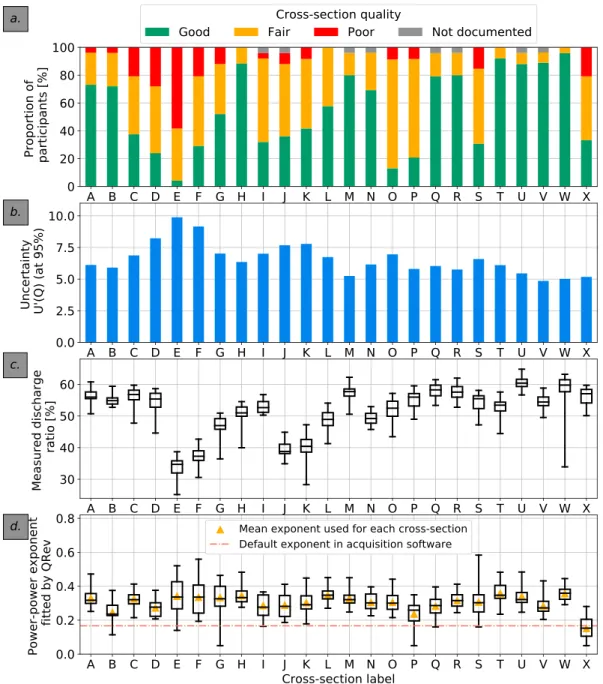
During the measurements, each team had to judge the quality of each cross section they measured as poor, fair, or good. More than half of the cross sections were considered as good cross sections and only 9% as poor. Figure 2 shows the quality evaluation for each cross section. It appears that cross-section E is considered as the worst cross section. This may be explained by the presence of a fallen tree upstream of the cross section.
Figure 2. Results obtained at the 24 cross sections (from upstream to downstream) of the Chauvan 2016 acoustic
Doppler current profiler experiments: (a) Quality assessment of measuring conditions. (b) Expanded uncertainty (at 95% level of confidence) of a single-transect discharge measurement based on one-way analysis of variance. (c) Boxplot of measured discharge ratio of six-transect averaged discharge measurements. (d) Boxplot of power-power exponent fitted by QRev on six-transect averaged discharge measurements. The boxes show the median, first, and third quartiles of the data, while the whiskers show the minimum and maximum values.
This cross section was also the shallowest (see transect E in Figure 1). More details regarding the general organization, site description, and experiment implementation are presented in Despax et al. (2017). 2.3. Experiment Implementation
Each team performed six-transect discharge measurements (three reciprocal pairs) at 12 of the 24 cross sections over the course of all three sessions. The experimental design is defined as balanced since the num-ber of repeated measurements (numnum-ber of transects) was set to 6 for each team at each cross section. For practical reasons (time constraints), a decomposition into two groups of cross sections was done, so that the experimental design is considered as crossed for each group, meaning that each team measured the dis-charge at the same 12 cross sections. Twelve cross sections (group 1: A, B, E, F, I, J, M, N, Q, R, U, and V)
by the other 24 teams. As a consequence, two distinct ANOVA were applied separately to the two groups of cross sections. Although two discharge measurements are missing for cross sections O and T (Group 2), the experimental design is considered as crossed and balanced for each group. The total number of six-transect discharge measurements is 574.
During measurement Session 1 (on 8 November 2016 from 14:00 to 17:15, local time) and Session 2 (on 9 November from 8:45 to 12:00), the discharge was released by turbo generators Numbers 1 and 2, respectively. During Session 3 (on 9 November from 13:30 to 17:00), the discharge was released directly by a dam spill-way resulting in a different discharge. However, streamflow was steady during each session as monitored by ADCPs deployed continuously and the three gauges along the reach (Despax et al., 2017). To analyze discharge estimates homogeneously regardless of the session, the corrected discharge ̂Qi,𝑗,mis defined as follows:
̂
Qi,𝑗,m=Qi,𝑗,m,p−(Q•••p−Q••••
)
(11) where Qi,j,m,pis the mth discharge measurement performed at cross-section j by the team number i during
the pth session, Q•••pis the mean of all discharge measurements performed during session p and Q••••=
14.76 m3/s is the averaged value of the discharge measurements during all the sessions. Equation (11)
assumes that no interaction between the session and the cross section and team factors occurs. Such an assumption is realistic since mean discharges over the session are similar (Q•••p=1 = 14.86 m3/s ;
Q•••p=2 = 15.63 m3∕s;Q•••p=3 = 13.82 m3/s). The error sources and the error model applied to the
corrected discharge are thereby supposed to be the same as for uncorrected discharge (equations (1) and (2)).
2.4. Quality Review of Raw Discharge Measurements and Choice of Extrapolation Model
Prior to the statistical analysis, a data quality review was performed using QRev software in batch (Mueller, 2016) to clean the data set from avoidable errors and to homogenize the discharge computations (there are some differences in the way in which discharge is computed between instrument manufacturers). QRev is part of routine procedures in USGS and also in some agencies around the world. The Extrap (Mueller, 2013) module of QRev was also applied to homogenize and optimize the various options for reconstructing unmeasured discharges in the near-surface and near-bed layers.
For the top and bottom unmeasured zones, an extrapolation model has to be selected to describe the velocity profile. The possible extrapolation models for the top layer are power fit, constant fit, or three-point linear extrapolation. The bottom fit can be based either on a power or no-slip model.
For top and bottom power fit, a power model is applied to extrapolate the unmeasured areas based on Chen (1989). The exponent, notated 1∕m′, refers to the power model that describes the velocity profile v(z) at elevation z above the bed
v(z) = v(h)(z h
)1∕m′
(12) where v(h) is the velocity measured at elevation h. In rivers, the exponent can range from 1/3 to 1/10 (Hauet et al., 2018).
The no-slip model fits a power curve through zero at the bottom (solid boundary) and through depth cells in the lower 20% of the flow. A constant fit for estimating the top discharge assumes that the velocity in the topmost valid depth cell is the mean velocity until the water surface. The three-point model allows to fit situations where wind or other effects significantly affect the velocity at the water surface, for instance. The choice of extrapolation model and exponent was left to the participants. Although the velocity profiles were different among the cross sections (see Figure 1), the default power/power model with a 1/6 exponent was consistently selected in situ by the participants for all measurements as proposed by the acquisition software. Only two teams applied QRev to adjust the exponent during the experiments.
Thus, a postprocessing using QRev was done for the application of Extrap tool for fitting vertical profile mod-els and exponents (Mueller, 2013) to the six-transect discharge measurements. Since ADCPs were deployed at the same rope, it is assumed that consistent hydraulic conditions prevail for a given cross section. For
Figure 3. Boxplot of corrected six-transect averaged discharges measured by the 48 teams (top) and at the 24 cross
sections (bottom). The models of acoustic Doppler current profilers are labeled with the team index (RP and SP denote RiverPro and StreamPro, respectively). The boxes show the median, first, and third quartiles of the data, while the whiskers show the minimum and maximum values. Groups 1 and 2 are represented in blue and red, respectively. that reason, a power/power model has been selected for all measurements with the average of fitted expo-nents at each cross section (Figure 2). The exponent ranges from 0.15 at cross-section X (1∕m′ ≈ 1∕6) to 0.37 at cross-section T (1∕m′ ≈1∕3). The mean exponent is 0.29 (1∕m′ =1∕3.4). This exponent denotes a typical rough riverbed (Welber et al., 2016) but seems to reflect the height of the roughness elements com-pared to the water height. Note that the sensitivity to the choice of the extrapolation model is not addressed completely in this paper but will be discussed further in section 3.4.
3. Results
3.1. Discharge Results and Investigation of Error Sources
Table 3 summarizes the statistics of water level at the hydrometric station and ADCP discharge measure-ments for each session. The standard deviation is 0.40 m3∕s. It corresponds to a possible change of ±1.5-cm
water level at the hydrometric station, that is the maximum standard deviation of water levels observed dur-ing the sessions (Session 2; see Table 3). Note that the small short-term fluctuations of water levels are not correlated in time and do no not reflect transient flow. Therefore, they would not affect the estimation of the systematic errors in equation (6). Instead, stage and discharge fluctuations can contribute to random errors (residuals). Similar mean discharges and standard deviations between the three sessions allow the use of the same error model (equation (1)) for the three sessions by correcting the discharge values fol-lowing equation (11). This assumption considers that the cross-section and team effects are the same in all three sessions.
group of 24 teams measured the discharge at 12 cross sections). The scatter within the two groups is equiv-alent although the two poorest cross sections (E and F; see Figure 2) are included in Group 1. Results in terms of corrected discharges depending on the team and on the cross section are shown in Figure 3. Most of the six-transect averaged discharges are within ±5% around the grand mean discharge (Figure 3). When considering discharges averaged by team, a maximum difference to the grand mean of ±4% is observed for teams 32 and 39 that are included in Group 2. However, these two teams were self-consistent, with a small scatter in measurements compared to other groups. These differences account for possible bias (systematic error) due to the team. It could be caused by an incorrect sensor draft setting, by the impact of the platform used or by incorrect shore distance estimation.
On the other hand, the mean discharges by cross section remain under ±1% around the grand mean (Figure 3). There is no significant bias observed among the cross sections, that is, no systematic overestima-tion nor systematic underestimaoverestima-tion. According to Figure 3, the systematic error associated with the cross section is lower than that associated with the team.
Additionally, the scatter among the 24 cross sections reveals the magnitude of random errors. For example, the discharges are less scattered for the most downstream cross sections (U, V, W, and X, with a standard deviation lower than 0.30 m3∕s), while discharges measured at cross-sections E and F are very scattered,
with a standard deviation of 0.50 m3∕s. Cross-sections E and F are located downstream of a weir yielding,
and they are shallow. They are also located downstream of a tree that affects the flow distribution and the free surface. Cross-sections U, V, and W where a larger fraction of the total flow area was measured show less scatter in the measurements (Figure 2). These cross sections were also rated by the operators as good (Figure 2). On the other hand, cross-sections E and F have a smaller measured discharge ratio, 35% and 40%, respectively. These cross sections are among the poorest according to operator evaluations (Figure 2). However, the quality evaluation was mostly rated after the measurement, whereas it should have been rated prior to the measurement to keep the rating independent of the results. The evaluation may have been influenced by the visualization of the cross-sectional geometry and water velocities or by the observed scatter of transect discharges.
The scatter of the six-transect discharge measurements may be explained by an interaction of both cross-section and team effects. The unmeasured area of the cross section or an error in edge distance esti-mation by the different operators leads to possible greater error that is magnified by a poor cross section with a low measured discharge ratio. For instance, the shallowness of the cross-section E makes discharges measured using ADCPs more susceptible to errors in ADCP draft and in bottom and top discharge estima-tions. Errors due to velocity profile extrapolation are magnified when the selected coefficient does not fit the vertical velocity profile or when the blanking distance is large relative to the cross-section depth.
Regarding cross sections where the near-bank unmeasured area is important (cross-section D, where 6% of the total discharge is extrapolated at the edge), the errors induced by the operators may be greater when using inappropriate distance-measurement device, when the boat is not kept nearly stationary near the bank (for obtaining an accurate mean velocity) or when setting an inappropriate edge-shaped coefficient (Mueller et al., 2013). At each cross section, the edge shape was assumed to be rectangular by half of the participants, while a triangular edge shape was used by the other participants. However, the choice of edge-shape coef-ficient played a limited role on the total discharge since only 1% is extrapolated near the edges for all other cross sections.
3.2. Uncertainty Analysis Based on a One-Way ANOVA
A one-way ANOVA was applied to the 574 six-transect discharge measurements processed with QRev and corrected for intersession discharge fluctuations. In this context, the factor is a laboratory which is the combi-nation of the operators, their equipment, and the measurement location (cross section). The equations used are presented in section 1.3. The results in terms of repeatability and interlaboratory standard deviation, sr
and sA, respectively, are presented in Table 4. The uncertainty related to the ADCP method bias is assumed
to be the same as previous experiments. Le Coz et al. (2016) estimated u( ̂𝛿) at 1.2%. It yields an expanded uncertainty of ±6.8% (at 95% level of confidence) for a one-transect measurement in the given measurement conditions of the experiments. The large number of participants leads to a robust uncertainty estimate with
Table 4
One-Way and Two-Way ANOVA Uncertainty Estimates for a Single-Transect Discharge Measurement
Sets sr sA sB sAB U(Q; at 95%) m3∕s % m3∕s % m3∕s % m3∕s % m3∕s % One-way ANOVA All data 0.31 2.1 0.39 2.6 — — — — 1.0 ±6.8 Two-way ANOVA Group 1 0.33 2.2 0.11 0.8 0.22 1.5 0.28 1.9 1.0 ±7.0 Group 2 0.30 2.0 0.14 0.9 0.26 1.8 0.25 1.7 1.0 ±6.9
Good cross sectionsa 0.27 1.8 0.18 1.2 0.20 1.4 0.14 0.9 0.9 ±5.8
Poor cross sectionsb 0.42 2.9 0.09 0.6 0.31 2.1 0.35 2.4 1.3 ±8.9
Note.In all cases, the uncertainty related to the bias,u( ̂𝛿), is estimated at 1.2%. ANOVA = one-way analysis of variance.
aCross-sections M, U, and V constitute the good cross-sections subset.bCross-sections E, F, and I constitute the poor cross-sections subset.
a 95% confidence interval between ±6.4% and ±6.9% (Le Coz et al., 2016). Considering six-transect mea-surements, the expanded uncertainty is ±5.6%, which is similar to the uncertainty assessed during previous repeated measures experiments in favorable conditions (see Table 1).
In addition, the one-way ANOVA was applied to two subsets considering the ADCP models. A subset of StreamPro ADCPs and a subset of M9 ADCPs were studied separately. Based on an equivalent number of measurements, the uncertainty estimates are ±6.7% and ±6.8% for StreamPro and M9, respectively (Despax et al., 2017). The similar uncertainty estimates between ADCP models suggest similar performance of the instruments used for these site conditions. Furthermore, since the mean discharges are similar (difference
≪ 1%), it also shows the absence of bias between the two ADCP models.
It is also possible to apply the one-way ANOVA to a subset of the discharge measurements. For example, the 24 discharge measurements performed at cross-section A constitute a subset. Applying the analysis to each cross section as a subset yields an uncertainty that ranges between ±4.9% and ±9.9% for cross-sections V and E, respectively (Figure 2). The cross-section V presents the highest measured discharge ratio while, cross-section E has the smallest ratio among all the cross sections.
The interlaboratory uncertainty component covers a large proportion of the total variance (57%), while the repeatability and the bias estimation uncertainties contribute a proportion of 38% and 5%, respectively. Note that the repeatability uncertainty is reduced when increasing the number of transects. The interlaboratory uncertainty is due to operators, instrument, and cross-section effects and possible interaction between these error sources. However, the method lumps these error sources together into one factor and does not allow further decomposition.
3.3. Estimation of Uncertainty Components (Two-Way ANOVA)
Since the cross-section (factor A) and team (factor B) effects are crossed in the experimental design, their respective contributions to the uncertainty are captured and can be estimated separately. Note that the effect of the cross section is fully isolated, while the other systematic effects due to the operators and the instruments are lumped. The application of a two-way ANOVA (computations presented in section 2.1) only estimates the uncertainty for a single-transect discharge measurement and yields the values shown in Table 4 for the two groups that both describe crossed and balanced experimental designs. The results are also given for two subsets of three cross-sections (M, U, and V) and (E, F, and I) that represent good and poor cross sections in Group 1, respectively. Note that the uncertainty estimates presented in Table 4 for the good and the poor subset are representative of cross sections with the largest and the smallest measured discharge ratio, respectively. Figure 4 shows the decomposition of the variance into each uncertainty component (s2
r, s2 A, s 2 B, s 2 AB, and u 2( ̂𝛿)).
The repeatability component is represented by the residual variance (s2
r) observed through the repetition
of transects. This component is the highest since the direct result of the ANOVA is the uncertainty esti-mate for a single measurement repetition. Single-transect measurement is not standard practice; hence, the repeatability component could be reduced by increasing the number of reciprocal transects in the aver-age, as recommended by general guidance for making ADCP discharge measurements (Le Coz et al., 2008;
Figure 4. Decomposition of the variance for four subsets of cross sections of the Chauvan 2016 experiments. Groups 1
and 2 are composed of 24 teams each ensuring a balanced and crossed experimental design. Cross-sections M, U, and V constitute a subset of good cross sections, while cross-sections E, F, and I are rated as poor. Those six cross sections belong to Group 1.
Mueller et al., 2013; WMO, 2010). In all cases, this component accounts for one third of total variance esti-mate and is not sufficient to predict the total uncertainty. The residual uncertainty (sr=0.31 m3/s) can be
fully explained by the short-term, uncorrelated stage fluctuations observed at the hydrometric station since the standard deviation of stage (1 cm) represents 0.30 m3/s.
The cross-section (s2
A) and team (s2B) components reflect systematic errors, or bias, when considering a single
team or a single cross section, respectively. The interaction between those effects (s2
AB) reflects other
system-atic errors specific to cross section/team pairs. The proportion of the uncertainty due to the cross-section effect is relatively small, between 2% and 17%, compared to the uncertainty induced by the team which ranges between 18% and 27% of total variance. Surprisingly, the cross-section component is higher for good cross sections than for poor cross sections, reflecting a higher deviation from the grand mean for the three good cross sections compared to cross-sections E, F, and I (see Figure 3). However, the poor cross-section subset results in a larger contribution of the component due to the interaction between the team and the cross section (29%, 0.35 m3/s).
3.4. Choice of Extrapolation Model
In the uncertainty estimates presented above, the choice of the extrapolation model is not taken into account since a power/power model with an exponent fitted for each cross section was consistently used. Three other alternative configurations were distinguished to analyze the impact of the extrapolation model using QRev software:
• A power/power model with a default 1/6 exponent (default exponent in acquisition software), • A power/power model with an individual exponent optimized for each six-transect measurement, • A fully automated processing (no constraints on the extrapolation model).
Considering a power/power model with an exponent optimized for each individual measurement (instead of for each cross section) does not affect the discharge estimates nor the uncertainty compared with the selection of an exponent fitted for each cross section. Although the optimized exponent computed by QRev ranges between 0.10 (1/10) and 0.45 (≈ 1∕2) among the 574 measurements (Figure 2), the standard deviation
Figure 5. Normalized velocity profiles for two measurements performed at the same cross-section M with a M9 (left)
and a StreamPro (right). The Extrap module of QRev fits a power/power model for the M9 measurement, while a constant/no-slip model is proposed for the StreamPro measurement. Red segments are not used in the computation of the extrapolation due to insufficient number of points.
of all discharge estimates is slightly higher (0.42 m3/s) than for an exponent fitted by cross section (0.40 m3∕s,
see section 3). Note that the overall discharge average remains the same (14.76 m3∕s). The use of the default
1/6 exponent proposed by the acquisition software does not impact the standard deviation (0.42 m3/s) but
reduces the mean discharge (14.71 m3/s). Discharges provided by the manufacturer software were almost
the same as the discharges computed in QRev based on a power-power model with a 1/6 exponent. However, some large errors were detected (e.g., transducer draft errors) and corrected thanks to QRev. Thus, QRev is useful to detect avoidable errors, hence decreasing the uncertainty.
On the other hand, the automatically selected extrapolation model (default method in QRev), based on Extrap tool (Mueller, 2013), leads to significant changes in discharge and uncertainty. In automated mode, the mean discharge is 14.53 m3/s and the standard deviation increases to 0.52 m3/s. The associated
uncer-tainty for a single-transect measurement reaches ± 8.3%. The increased variance is explained by the fact that power/power or constant/no-slip models may be selected by QRev as extrapolation models. Over all the six-transect discharge measurements, a 75%/25% proportion between power/power and constant/no-slip models is observed. For some cross sections (D, P, S, and T), the proportion between the two models is 50%/50%, while the model selected should be the same due to identical hydraulic conditions. The varia-tion between the two models selected is directly linked with the ADCP models distribuvaria-tion (remember that StreamPro and M9 ADCPs were spread evenly among the cross sections). For most of StreamPro measure-ments, QRev automatically selected a constant/no-slip model, while M9 measurements were assigned a power/power fit (see Figure 5). For M9 measurements, data acquired within 16 cm of the transducer are automatically marked invalid by QRev, due to possible flow disturbance induced by the instrument and its float (Mueller, 2015; Muste et al., 2009). This excluded distance is set to 16 cm for M9, while it is set to zero for all other ADCPs. Most of StreamPro ADCPs were mounted on trimaran, whereas M9 ADCPS were mounted on board which may cause flow disturbance near the water surface. As a result, the vertical velocity profile fitted for StreamPro measurements seems to be constant near the surface, while the excluded data do not allow to assess correctly the shape of the curve for M9 data (see Figure 5). However, the model fitted on StreamPro data may also be affected by errors, including those resulting from flow disturbance, although no flow disturbance was observed by Mueller (2015). In the experiments, the variability of discharges is mostly explained by the top unmeasured area. Its contribution to the total discharge ranges between 15% and up to 50% for the shallowest cross sections measured with a M9 ADCP (cross-section E). In these configurations, the difference in discharges between a constant profile and a 1/3 power fit is magnified. The change of the
Figure 6. Expanded uncertainty (at 95% level of confidence) of a discharge measurement as a function of the total
number of transects: (left) for one team measuring at several cross sections and (right) for several teams measuring at a single cross section. The team and the cross section are representative to those involved in the experiment.
extrapolation model is induced by the use of distinct ADCP models and therefore affects both sB(team) and
sAB(interaction) components.
Lastly, the difference in mean discharge between power/power fit or automatically selected extrapolation suggests a possible bias due to the choice of extrapolation model. The bias magnitude is 1.5%, while the difference between power/power model with a default exponent (1/6) and with a fitted exponent is 0.3%. 3.5. Transect-Averaged Discharge Uncertainty
Equation (10) gives the expanded uncertainty as a function of the number of cross-sections a, the number of teams b, and the number of transects n used to estimate the discharge. Figure 6 shows the uncertainty as a function of the total number of transects. Two configurations are distinguished. The first considers transects distributed across different numbers of cross sections (from 1 to 4) performed by one team (b = 1, which corresponds to operational conditions), while the second configuration gives the uncertainty for transects that are distributed at a single cross section (a = 1) but performed by several teams (from 1 to 4). The team and the cross section considered here are representative of those involved in the experiment. Thus, the results are given for an average team and an average cross section. The total number of transects is analogous to the duration of the measurement. In this experiment, the mean duration of one transect is 120 s. Thus, a six-transect measurement lasts for 720 s which corresponds to USGS standard procedures (Oberg & Mueller, 2007).
For a given total number of transects (i.e., the same total measurement duration), exploring more cross sections is more efficient to reduce the uncertainty than staying at the same cross section. For instance, eight transects performed at one cross section by one team lead to an uncertainty of ±5.7%, while averaging two measurements performed at two cross sections using four transects each (total number of transects of eight) gives an expanded uncertainty of ±4.9%.
As expected, from one to two teams the uncertainty decreases notably, but from two to three teams the reduc-tion is limited since the uncertainty is decreasing with the square root of number of teams (a) according to equation (10). Considering discharge measurements performed with a total of abn = 8 transects, averaging two measurements performed at a = 1 cross section by b = 2 teams is slightly more efficient to reduce the uncertainty than averaging discharge measurements operated by b = 1 team at a = 2 cross sections (±4.5% and ±4.9%, respectively). Averaging four two-transect measurements performed at a = 2 cross section by
stabilizes fairly rapidly when a or b increase. This is consistent with above-mentioned observations that the possible bias observed for a given team in Figure 3 could be decreased when averaging the discharges mea-sured by two or more teams. Bias from a single cross section is much smaller than bias from a single team. Thus, the decrease in uncertainty from averaging multiple cross sections is proportionally smaller than the decrease when averaging multiple teams. Considering several teams measuring the discharge at multi-ple cross sections reduces even further the uncertainty since the dominant uncertainty component (s2
AB) is
reduced. However, in operational conditions, averaging the discharges performed by one team (b = 1) at multiple cross sections remains significant to reduce the uncertainty as the team/cross-section interaction uncertainty will also decrease.
4. Discussion
4.1. General Recommendations for Reducing Systematic Errors 4.1.1. Systematic Errors Due to the Cross Section
As suggested by Figure 6, a recommendation in order to reduce the uncertainty may be to select several equally good cross sections to perform a discharge measurement. For a given cumulative number of transects (same total measurement duration), exploring more cross sections is more efficient to reduce the uncertainty than staying at the same cross section and increasing the number of transects. The systematic errors related to the cross section (i.e., bias for a single cross section) due to effects such as ambient turbulence or channel features (aspect ratio, channel sinuosity, and bed singularities) may be reduced by averaging out over two or more cross sections. At least one reciprocal pair of transects must be measured at each cross section to average out any directional bias, as recommended by best practices (Mueller et al., 2013).
4.1.2. Systematic Errors Due to the Team
Figure 3 and Table 4 show that the systematic errors due to the team are larger than the ones due to the cross section. The operator-induced bias error may include incorrect sensor draft setting and poor choice of edge-shaped coefficient (Simpson, 2001).
Thus, gathering two teams appears to be even more efficient than exploring multiple cross sections to reduce the expanded uncertainty. In this case, all systematic errors due to the team (i.e., bias for a single team) such as draft or edge estimate models are averaged out and reduced. When multiple instruments are used, the instrument bias for a single measurement also becomes a random error and is thus reduced by the average. However, gathering two—or more—teams is costly and more complex operationally.
4.1.3. Systematic Errors Due to Interactions
The results also suggest that the various choices made to extrapolate unmeasured areas (see section 3.4) or an error in edge distance estimation by the different operators may magnify the error when the quality of the cross section is poor (small measured discharge ratio or unusual vertical velocity profile for instance). The systematic errors due to interactions represent a bias associated to the combination of a single team and a single cross section. The bias may be reduced by averaging out over two or more teams at two or more cross sections.
Although the interaction between team and cross section is strong, the influence of the effect of the team seems to be more important than the choice of the cross section itself as long as the general rules and guid-ance for making ADCP discharge measurements are followed. Table 5 proposes a list of the operator-induced errors that may cause interaction with cross-section errors. Fortunately, these errors are generally minimized when the measurement is performed by skilled operators and by conforming to the best practices (Simpson, 2001; Oberg et al., 2005). For instance, the use of an appropriate measurement device for estimating edge distances will decrease the uncertainty associated with the edge discharge extrapolation.
Special attention must also be paid to the selection of an appropriate model for the top and bottom extrapo-lations. Although a default power/power fit with 0.1667 (1/6) exponent is commonly used, the extrapolation model and its associated exponent should be adjusted to fit the measured data. To address possible bias when the blanking distance is an important factor, an independent measurement—performed with a cur-rent meter or a surface velocity measuring instrument—could be used to help select the most appropriate extrapolation model (between power/power and constant/no-slip model for instance).
It could also be beneficial to perform a trial transect prior to starting a measurement as suggested by the USGS procedures (Mueller et al., 2013). Collecting one or several stationary velocity profiles at the cross section would also help to capture any variability in the velocities. These preliminary measurements provide
Table 5
Operator-Induced Errors That May Cause Interaction With Cross-Section Errors
Category Error source Variable affected Covered in Chauvan 2016 tests
Settings (instru- Selection of water profiling mode Total discharge Active (mode 12 used for Teledyne RDI
ment and processing instruments, default modes otherwise)
configuration)
Navigational (GPS or bottom track) and depth Total discharge Not active (bottom track and four-beam
(vertical beam or four-beam average) reference average used)
Cell size Total discharge Active
Edge-shaped coefficient Edge discharge Active
Invalid data and extrapolation Interpolated and Not active (QRev processing with
extrapolated discharge same configuration)
Other configuration Total discharge Active
Operating ADCP model or frequency (range limitations), float Total discharge Active (board or trimaran was used) Sampling measurement time (and spatial time) due to Total discharge Active
boat navigation
Edge sampling Edge discharge Not active (10 pings in stationary
position near the edges)
Boat navigation Total discharge Active
Measurements Edge distance measurement Edge discharge Active
Sensor draft Top discharge Active
Operator skills Choice of the cross section (backwater, importance of Total discharge Active flow inhomogeneity, proportion of invalid data,
shallow depths, large turbulence intensity,
and no vegetation) QA/QC procedure (software and Total discharge Not active (recent software and firmware firmware, moving bed test, independent temperature version used, fixed bed, consistent
checking, and compass calibration) temperature among instruments,
bottom track reference used)
ADCP mounting Total discharge Active
Note.The last column indicates whether the error was active during the Chauvan 2016 ADCP field experiments. ADCP = acoustic Doppler current profiler.
an insight into the velocity field and into the depth across the river in order to select an appropriate water mode profiling, to adapt the boat navigation, and to set appropriate parameters for estimating the unmea-sured portions. Indeed, the selection of an appropriate cross section is the key to significantly reduce the sensitivity to the choice of the extrapolation model, to the boat positioning at the start/end edge, and to the parameters used.
4.2. Generality of the Results
Although the uncertainty estimated with repeated experiments is specific to the study site and to the instru-ments and operators involved, the results suggest a range of uncertainty estimates for poor and good cross sections that can be used in other studies. At the same studied site with a higher flow rate, we can expect that the impact of unmeasured areas might be reduced due to a smaller relative proportion of extrapolated discharge. It might reduce the standard uncertainty of cross-section effects and their interaction with the team effects.
As shown by the comparison of uncertainty estimates based on two subsets of instruments (section 3.2), the impact of the instrument appears to be negligible between the models tested: M9 and StreamPro, for the flow conditions studied (1-m depth, 0.50 to 0.75-m∕s mean velocities). This result is in line with performance tests conducted by Boldt and Oberg (2015). Hence, the uncertainty associated with the team factor may be assumed to represent the operator uncertainty alone. Given the number and the diversity of operators gathered in the experiments, the standard uncertainties sBprovided in Table 4 may be assumed to reflect the uncertainty of typical field hydrologists.