A device user interface for the guided ablative therapy of cardiac arrhythmias

I

A DEVICE USER INTERFACE FOR THE GUIDED ABLATIVE

THERAPY OF CARDIAC ARRHYTHMIAS

by

Maya Barley

B.S., Electrical Engineering Rice University, 2001

Submitted to the Department of Electrical Engineering and Computer Science in Partial Fulfillment of the Requirements for the degree of

Master of Science in Electrical Engineering

at the

_8ARKER

Massachusetts Institute of Technology

August 2003

© 2003 Massachusetts Institute of Technology All rights reserved

The author hereby grants MIT permission to reproduce and distribute publicly paper and electronic copies of this thesis document in whole or in part, and to grant others to do so.

Signature of Author

Depattment of Electrical Ergfnieering and Computer cience August 1, 2003

Certified by

Richard J. Cohen, M.D., PhD. Whitaker Professor in Biomedical Engineering,

MASSACHUSETTS INSTfITUTE OF TECHNOLOGY

FMA

6R2006

A Device User Interface for the Guided Ablative Therapy

of Cardiac Arrhythmias

by Maya Barley

Submitted to the Department of Electrical Engineering and Computer Science on August 1, 2003 in Partial Fulfillment of the Requirements for the Degree of

Master of Science in Electrical Engineering

ABSTRACT

Radio Frequency Ablation (RFA) of cardiac arrhythmias involves the guidance of an ablation catheter to the site of the arrhythmia and the administration of a high-intensity radio-frequency current to the tissue. The current technique used to locate the arrhythmic site suffers from a number of drawbacks. Ablation is a trial-and-error procedure and may require many hours, during which the arrhythmia is ongoing. Patients with hemodynamically unstable VT are therefore excluded, as are those with more complex arrhythmias, accounting for an estimated 90% of patients. Furthermore, the technique is only successful in 71 % to 76% of the cases to which it is applied.

A new algorithm was recently identified that allows the non-invasive and rapid detection of the origin of an arrhythmia from body-surface ECG signals, making the RFA procedure accessible to many patients hitherto excluded. Software implementing this algorithm, and providing a multi-layer graphical user-interface to operate in conjunction with an RFA device, has been designed and implemented. If used in tandem with commercially available ECG and ablation catheter devices, this software will allow cardiologists to deliver ablating currents much more precisely and more quickly than is currently possible, and reach a far wider group of patients.

Thesis Supervisor: Richard J. Cohen, MD, PhD. Title: Professor of Health Sciences and Technology

Acknowledgements

First, I would like to thank Dr. Cohen for his support, help and patience through all this work.

I also want to thank Dr. Bill Stevenson for kindly allowing me to sit in on an ablation procedure and answering all my questions.

Thanks also to Dr. Stephen Burns for helping to get me started on this project, to Antonis for patiently putting up with all my questions about the inverse algorithm while he was trying to work, and to Grace and Tamara, two wonderful lab-mates who have given me advice and guidance.

I want to thank my parents for all their love and never-ending support (and highly useful advice).

And Adrien for always being there for me, always encouraging me to do more than I thought possible, and making my life wonderfully happy.

Table of Contents

1. CLINICAL BACKGROUND ...

7

1.1 C ardiac A rrhythm ias ... 7

1.1 .1 C au se s ... 7

1.1.2 Re-entrant Circuit Formation ... 7

1.2 Current Treatment for Arrhythmias ... 8

1.2.1 A ntiarrhythm ic drugs ... 8

1.2.2 Implantable Cardioverter-Defibrillators ... 9

1.3 R adio-Frequency A blation ... 10

1.4 Current Endocardial Mapping Techniques ... 11

1.4.1 Mapping of Hemodynamically Stable Ventricular Tachycardia... 11

1.4.2 Mapping of Hemodynamically Unstable VT ... 14

1 .4 .3 A b latio n ... 15

1.4.4 Probability of Success ... 15

1.5 New Mapping Technologies ... 16

1.5 .1 C A R T O ... 16

1.5 .2 E n site 3000 ... . 16

1.5.3 Body Surface Potential Mapping ... 17

2.

A NEW METHOD: THE INVERSE TECHNIQUE ...

18

2.1 Solving the Inverse Problem ... 18

2.2 Mathematical Basis for the Inverse Algorithm ... 19

2.3 Benefits of using the Inverse Algorithm as a Mapping Tool ... 19

3.

DESIGN OF THE RFA DEVICE...

21

3.1 Overall RFA system design ... 21

3.1.1 Locating the re-entrant circuit ... 21

3.1.2 Guiding the Ablation Catheter ... 22

3.2 Biomedical Safety Considerations ... 23

3.3 Choice of Operating System and Software ... 23

4.

THE GRAPHICAL USER INTERFACE...25

4.1 U ser Interface Structure ... 25

4.2 U ser Interface Specifications ... 25

4.3 Choice of Programming Environment ... 28

4 .4 D ata S ou rces ... 2 9

5.

SIGNAL ACQUISITION AND DISPLAY... 30

5.1 Patient Inform ation Entry... 30

5.2 The Data Acquisition Interface ... 32

6.

SIGNAL PARAMETER AND DIPOLE ESTIMATION... 41

6.1 Matlab Program Structure for Dipole Parameter Calculation... 41

6.2 Signal Parameter Estimation ... 42

6.2.1 B aseline E stim ation ... 42

6.2.2 High-frequency Noise Estimation ... 49

6.2.3 Selecting high-quality channels... 51

6 .3 D ipole E stim ation ... . . 5 1

7.

DIPOLE VISUALIZATION ...

53

7.1 Structure of dipole visualization software... 53

7.3 Selecting the dipole of interest... 58

7.4 The Ablation Interface: Simultaneous display of dipole and ablation catheter ... 59

8.

THE CHOICE OF ABLATION SITE...61

8.1 Position in ECG waveform and within the dipole trajectory ... 64

8.2 D ipole A m plitude... . 65

8.3 Distance between consecutive dipoles ... 65

8.4 Chi-square and RNMSE... 65

8.5 The Positional Uncertainties in x, y and z... 66

8.6 Which dipole best represents the exit point?... . . . .. . . .. . . . .. . . . .. . . . .. . . . 67

9.

CONCLUSIONS AND FUTURE WORK...69

10.

REFERENCES ...

71

APPEN DIX A . ...

74

APPENDIX B . ...

76

APPENDIX

...

77

1. Clinical Background

Cardiac arrhythmias - changes in the regular beat of the heart - are one of the most prominent causes of morbidity in the developed world. It is estimated that 200,000 people a year are treated for ventricular arrhythmias. Furthermore, of the 700,000 deaths each year caused by heart disease in the United States, 60% to 65% are sudden and presumed to be caused by tachyarrhythmias. [1]

1.1.1 Causes

There are several underlying causes of tachycardia. Non-ischemic dilated cardiomyopathy, hypertrophic cardiomyopathy, valvular disease, regional autonomic dysfunction [2] , congenital heart disease and primary electrophysiological abnormalities (such as Wolff-Parkinson-White Syndrome) are all contexts for ventricular tachyarrhythmias. However, eighty percent of sudden cardiac deaths attributed to arrhythmias are due to the after-effects of a myocardial infarction.[3] The electrical properties of infarcted tissue can cause the formation of a reentrant circuit and the precipitation of a lethal ventricular tachycarrhythmia. These regions can also become points of abnormal initiation of impulse activity. Transient myocardial ischemia, perhaps caused by coronary spasm or unstable platelet thrombi, can lead to death via the same mechanisms. [4]

1.1.2 Re-entrant Circuit Formation

As stated above, the conduction properties of infarcted tissue can result in the formation of a re-entrant circuit, a form of abnormal impulse conduction.[5] Figure 1.1 shows a theoretic reentry circuit originating from a chronic infarct. A normal sinus rhythm beat, sweeping through the myocardium to depolarize the entire ventricle, encounters the entrance site of the reentrant circuit. If the circuit 'captures' during this QRS complex, the entrance to the scar region is also activated and a wavefront propagates slowly through the scar tissue. At the exit point, it emerges from the infarct region into normal tissue. If the conduction time from entrance to exit within the scar exceeds the refractory period of the functioning myocardium, this will cause the onset of a second

site. If the speed of conduction is very fast, a rapidly circulating wavefront or 'circus rhythm' is initiated, and ventricular tachycardia results.

A

Outer Loop QRS Onse

Figure 1.1: Reentrant Circuit around an infarct scar. From Stevenson at al. [21]

1.2 Current Treatment for Arrhythmias

1.2.1 Antiarrhythmic drugs

Antiarrhythmic drugs are frequently prescribed because they alter the electrophysiological properties of the reentrant circuit and suppress potential triggers for the development of VT.[6] However, within 2 years, > 40 % of patients being treated for sustained VT will experience recurrences. [7] Also, an antiarrhythmic drug can create an abnormality on which a transient risk event, such as ischemia, interacts to produce a lethal ventricular arrhythmia. [8]

This was clearly demonstrated in the Cardiac Arrhythmia Suppression Trial (CAST). CAST showed that despite the increased risk of sudden cardiac death associated with ventricular ectopic beats, in post-infarction patients and older age groups, suppression of these arrhythmias with class I drugs such as encainide and moricizine, calcium antagonists, and class III drugs conferred either an increased risk of death or no improvement on survival. [9] It is hypothesized that the negative dromotrophic actions of these drugs exacerbated ischemia-induced conduction slowing. Thus, a transient change in the myocardial substrate could cause anti-arrhythmic drugs to actually become a risk factor for sudden cardiac death.

Only Amiodarone and beta-blockers have been shown to generally decrease the risk of sudden death in the myocardial infarction patient. However, amiodarone produces side effects in 75% of patients within 5 years, including hypothyroidism, tremor and neurological toxicity. Clearly, a more effective means of treating ventricular arrhythmias is needed.

1.2.2 Implantable Cardioverter-Defibrillators

Three recent studies confirm the superiority of implantable cardioverter defibrillators (ICDs) over antiarrhythmic drug therapy for preventing sudden death in patients at risk for hemodynamically unstable ventricular tachyarrhythmias. [10], [11], [12] These devices can administer anti-tachycardia pacing that will terminate most monomorphic VTs, and electrical cardioversion if necessary. During cardioversion, a single high-energy pulse of current is administered to the heart, 'resetting' the cycle of electrical activity; it is hoped that once the tissue is uniformly de-polarized, normal sinus rhythm will resume.

Approximately one third of patients will experience some adverse effect, including inappropriate shocks, lead problems, and infection. [1 3] The 'shock' of cardioversion felt by ICD patients is substantial and there are many instances of patients either requesting that the device be removed or refusing implantation. [14] Often, amiodarone is used in conjunction with an ICD since it reduces the frequency of cardiac events necessitating defibrillation. However, antiarrhythmic drugs can lower the rate of VT to just below the ICD's threshold of detection or raise the energy required for defibrillation, reducing the probability that the ICD will be effective. Furthermore, ICD implantation and maintenance is expensive; the MADIT study found the average cost to be $27,000 per patient. [15]

Although ICDs extend survival, they only treat arrhythmias when they occur and do not prevent recurrences. [16] A form of preventive treatment is therefore desirable for cases in which the VT is persistent. The most recently developed procedure for the treatment of arrhythmias is radio-frequency ablation (RFA). It involves the guidance of an ablation catheter to the exit site of the reentrant circuit and the administration of high-intensity radio-frequency current to the tissue. If the site has been accurately identified and ablated, the necrotic tissue that remains will transect

therapies in 21 patients with any VT decreased from 59.3 ± 79.7 per month before ablation, to 0.6 ± 1.1 per month after successful ablation; this represents a 99.8% reduction in defibrillator therapies. These patients reported a significant improvement in quality-of-life after successful ablation.

1.3 Radio-Frequency Ablation

At the beginning of the procedure, ablation and electrode catheters are inserted into either a femoral artery or vein, depending on the location of the arrhythmic site suggested by the morphology of the VT, and advanced into the heart. The catheter positions are monitored with biplanar fluoroscopy (a 2-D imaging technique allowing 'real-time' x-ray), with 300 right anterior

oblique and 60' left anterior oblique projections. To remove positional changes due to heart motion, the fluoroscopic images are usually R-wave gated. A detailed map of endocardial electrical activity is produced using techniques defined below. Throughout the mapping procedure, the patient is administered 1000 units/hour of intravenous heparin to prevent

coagulation and thrombus formation around the catheters.

Once the site of the arrhythmia is determined from this map, fluoroscopy is used to guide the ablation catheter to the same site and the ablating current is delivered. The frequency of the current used is between 300 and 750 kHz, with a power output of 20 to 50W over a 30 to 90 second period. Irreversible tissue destruction requires a temperature of approximately 50 'C; therefore the power output of the radio-frequency generator is automatically or manually titrated to achieve a temperature between 60 and 75 'C. If the temperature at the catheter tip exceeds I

00

Typical ablation catheters are 2.2 mm in diameter and create a lesion 5-6 mm in diameter and 2-3 mm deep. The lesion consists of a central core of necrotic tissue surrounded by a zone of

hemorrhage and inflammation. The inflammation may resolve without residual necrosis, therefore if the reentrant exit site lies on the periphery of the lesion the arrhythmia could recur even several weeks after ablation. [18] Consequently, the ablation must be accurate to within one to two millimeters of the arrhythmic site to ensure success.

1.4 Current Endocardial Mapping Techniques

1.4.1 Mapping of Hemodynamically Stable Ventricular Tachycardia

induce

S~nns Rhythm Map

t enfec at sion .b s.a

NoM

Figure~~~~~~~~~O^ 1.:FoWiga fapoc OOpigad"baino"VSeia tal[1

Iniia VTp inductiony

Th sqene fmapigan bltinfo bt salean nsabeVTi sow n igr 12 VT~~~~~~~4 isfrs ndcd yri pacing detrieissraeQSmrpooywh rhtmai

then~~~~~~~~~5"S temntduigcrIvrino" us aig

Sinus Mawninw

Next, the electrical characteristics of the endocardial surface of the heart are mapped during sinus rhythm. This is done by consecutively stimulating the endocardium at over 500 sites using an

intracardiac electrode and recording the local bipolar electrograms. Observations of animal MI models suggest that reentry circuit isthmuses can be best defined by delineating infarcted areas of

dense, fibrous scar, since these are potentially arrhythmogenic. [19] The sinus mapping procedure identifies scar tissue by stimulating the endocardium sub-threshold while sinus rhythm is

ongoing. The resulting local electrograms are measured a few millimeters from the pacing electrode. Scar regions are characterized by low-voltage (< 1.5 mV) multiphasic electrograms. Slow conduction, suggested by a long delay between a supra-threshold pacing stimulus and surface QRS onset, is also indicative. Therefore, scar regions are termed zones offragmentation.

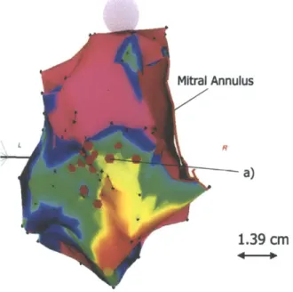
An example of an electroanatomical map produced by sinus mapping is shown in Figure 1.3.

Mitral Annulus

F?

1- a)

1.39

cm

Figure 13: Sinus Mapping. Colors indicate sinus rhythm electrogram amplitude, with lowest-amplitude areas of red, increasing to yellow, green amd blue. Normal voltage electrogram regions (> 1.5 mV) generated by 'healthy' endocardium are shown in purple. From Soejima et al. [21]

12

Pace Mapping

Pace-mapping to mimic the VT is then carried out. This technique is based on the principle that

supra-threshold pacing at the site of arrhythmic origin would result in an identical surface ECG morphology to that of the clinical VT. [20] By comparing and finally matching the QRS morphologies, the cardiologist can localize the site of reentry. For scar-based reentrant circuits, the mapping takes place along the border of the scar region to identify the exit point of the arrhythmia. Movement of the catheter from the exit site into the scar tissue itself demonstrates abnormal low-voltage electrograms and a supra-threshold pacing morphology similar to the VT morphology (often with a significant delay between stimulus and QRS).

Entrainment mappin!

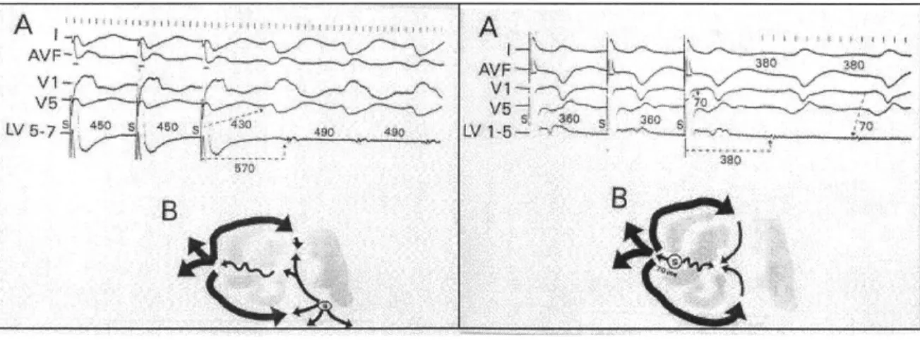
Finally, entrainment mapping is the gold standard for ablating hemodynamically stable reentrant circuits. It is carried out after pace-mapping has localized the site of the arrhythmia, and is used to identify the exact location. Figure 1.4 illustrates the principles of entrainment.

A

A

V F

Figure 1.4: Entrainment Mapping. The left illustration shows the ECG resulting

from

long

VT cycle length (490 ms), and the difference in

QRS

illustration

While the VT is ongoing, an endocardial site is paced at a cycle length 40 to 100 ms shorter than that of the VT. Unless the site is remote to the reentrant circuit, this results in acceleration of the VT to the pacing cycle length. If the site is not within the reentrant circuit, the post-pacing

interval - the time from the last pacing stimulus after pacing is stopped until the subsequent depolarization at the pacing site due to 'return' of the activation wavefront - will be more than 30 ms greater than the VT cycle length, as seen in Figure 1.4. This difference results from the addition of conduction time from pacing site to reentrant circuit and back to the conduction time through the reentrant circuit itself.

If the pacing site lies within the reentrant circuit, there is no significant conduction time between pacing site and reentrant circuit. However, pacing at a cycle length significantly shorter than the VT transiently alters the intracellular ionic composition of the myocytes. This changes the conduction properties of the cardiac tissue; therefore, a post-pacing interval within 30 ms of the VT cycle length is accepted.

When pacing occurs within the reentrant circuit, the collision of the pace-stimulated antidromic wavefront and the orthodromic wavefront (returning through the circuit) occurs near the pacing site. Since the antidromic wavefront depolarizes only a small section of tissue, this is not detectable on the surface ECG and the fusion of the two wavefronts is concealed [21]. This is

called entrainment with concealedfusion. Ablation at such a site will result in termination of the

tachycardia.

1.4.2 Mapping of Hemodynamically Unstable VT

It is impossible to sustain patients with more severe, hemodynamically unstable arrhythmias for the 3 to 6 hours in which VT is ongoing during entrainment mapping. [17] Instead after initial VT induction, the arrhythmia is quickly terminated. Sinus mapping is used to identify scar regions, and pace-mapping distinguishes sites at which the paced QRS morphology matches that of the unstable VT. Since pace-mapping is far less accurate than entrainment mapping, ablation in patients with unstable VT is generally unsuccessful and therefore rarely attempted.

1.4.3 Ablation

During ablation, a line of RF lesions is created in an attempt to transect the isthmus through which abnormal beats are transmitted to the functioning myocardium. In patients with reentrant circuits originating from MI scar regions, ablation lines follow the contours of the scar. The procedure is considered successful if the original VT is no longer inducible.

1.4.4 Probability of Success

The current probability of RFA success in a patient with purely monomorphic, stable VT is 71 to 76%. However, it is likely that this represents <10% of the total population of patients with VT. [22] Although Furniss et al. [23] have conducted a limited study indicating that RFA can be used to successfully treat patients with hemodynamically unstable arrhythmias, these patients are not generally treated unless their arrhythmia is incessant. In these cases, ICD implantation is considered the most appropriate option.

The extended duration of the procedure also exposes cardiologists and patients to undesirable levels of x-ray radiation. Furthermore, since fluoroscopic imaging of the heart yields a two-dimensional projection of a 3-D structure, it is difficult for the cardiologist to accurately gauge the catheters' positions in three-dimensional space. The LocaLisa system is a newly developed, non-fluoroscopic technique to localize the 3-dimensional position of ablation electrodes. It has been shown to yield reproducible results with an accuracy to less than 1.4 +/- 1.1 mm [24]. However, this system does not map the arrhythmia itself, therefore the overall accuracy of the ablation procedure is still limited.

Lastly, it is theoretically desirable to limit the number of ablation sites to the minimum required for success, minimizing the risk of damage to functioning myocardium and the creation of potentially thrombogenic endocardial lesions. [25] Current treatment may create upward of thirty lesions, and achieves only limited success.

1.5 New Mapping Technologies

1.5.1 CARTO

Two types of activation-mapping technology currently exist for use in radio-catheter ablation. 'CARTO' uses a special catheter to generate 3-D electroanatomic cardiac maps, and is now widely used in RFA procedures. A device external to the patient's body emits a very low

magnetic field that is detected at the tip of the mapping and ablation catheter, and is used to sense its location and orientation. The catheter tip simultaneously stimulates the cardiac tissue and records the resulting local electrocardiograms. The amplitude of the local electrograms during sinus mapping, and the site at which they were recorded, are displayed in a 3-D electro-anatomical map (as shown in Figure 3) that clearly delineates scar tissue. During pace and entrainment mapping, CARTO allows the cardiologist to mark sites on the map that demonstrate concealed fusion or a QRS morphology matching that of the VT. The catheter tip is also

displayed; the display is R-wave gated so that movement due to heart motion is cancelled.

As with the multiple lead imaging technique, CARTO has several drawbacks. Mapping is time-intensive therefore hemodynamically unstable patients are still untreatable. Also, the degree of resolution of the endocardial map is limited by the time available to acquire data points (upwards of 550 electrograms are required during ventricular mapping). The 3D map is not provided in real-time therefore new maps must be generated to detect a change in the arrhythmia or to fully-visualize multiple VTs. Lastly, multiple-point acquisition has to be performed with care, ensuring that contact with the endocardium is adequate and that fibrous, low-voltage structures such as the mitral valve annulus are appropriately delineated. Otherwise, scar-regions can be falsely

exaggerated. [20]

1.5.2 Ensite 3000

Another recent development is the Ensite 3000 basket catheter, a mapping system that uses a single, non-contact intra-cavity multielectrode array to sense the voltage field produced by endocardial activation. The 64-electrode braid array computes virtual electrograms

simultaneously from more than 3000 ventricular sites using a boundary element inverse solution. This information is then used to reconstruct the entire chamber's endocardial activity, which is displayed as a dynamic three-dimensional isopotential color map.

This is undoubtedly the best currently-developed mapping technique for complex or

hemodynamically unstable arrhythmias, and has shown success in several studies. [27] However, the overall accuracy of reconstructed electrograms decreases with distance from the electrode array affecting the validity of the map. [28] Also, the endocardial geometry that is used to calculate the boundary element inverse solution during VT is acquired during baseline rhythm; the assumption that the geometry does not change may be an important limitation if the heart is vigorously contracting. Furthermore, aggressive anticoagulation measures must be taken which can lead to serious bleeding complications. The Ensite 3000 is not widely used within the medical community.

1.5.3 Body Surface Potential Mapping

This is the only non-invasive mapping technology currently available, and is not widely used. An array of 64, 128 or 256 electrodes is placed on the torso, and the body surface potentials are recorded. The potentials on the heart surface are then computed by solving Laplace's equation within the torso volume, assuming a specific geometric relationship between the epicardial and torso surfaces. A dynamic isopotential map is then created which shows the spread of activation across the ventricles. By pacing at different sites within the ventricle, a database of isopotential activation maps is generated. By comparing the VT isopotential map to those in the database, the computer guides the catheter to the correct site for ablation.

Several studies have shown that BSP mapping is effective at imaging reentry pathways and their key components. [29] By improving the accuracy of reentry site identification, this mapping technique can also reduce the number of ablations required to terminate the VT. [30]

Furthermore, this system can reconstruct epicardial electrophysiological information, unlike CARTO and Ensite 3000. Since the sub-epicardium plays an important role in the maintenance of reentry circuits in up to 33% of patients, this is an important advantage.

However, in a study done by SippensGroenewegen [31], BSPM was found to localize the site of the arrhythmia only to within 2 cm of a pace-mapping site. Since an ablation lesion is only 5 to 6 mm in diameter, this degree of localization is insufficient. Also, BSPM has a limited ability to

suggested that BSPM be used for screening purposes or to examine the effect of certain

medications on the arrhythmic substrate, rather than as a mapping tool in RF ablation procedures.

2.

A New Method: The Inverse Technique

2.1 Solving the Inverse Problem

The Inverse Problem in electrocardiography involves the mapping of two-dimensional body-surface potentials to the three-dimensional cardiac excitation pattern that created them. The endocardial excitation pattern at any instant can be visualized as a wavefront of single electric dipoles. This is approximated as a belt source with a constant dipole moment per unit length directed parallel to the propagation direction. By summing the individual dipoles, the source can be approximated as a cumulative single equivalent moving dipole (SEMD). Therefore, the solution to the inverse problem is the SEMD that best reproduces the electrode potentials at a given set of electrodes at a given time instant.

In general, the inverse problem has no unique solution. Furthermore, it has been shown that a single equivalent point dipole source cannot adequately represent cardiac electrical activity throughout the cardiac cycle. [32] However if the source is well-localized, as is the case when the wavefront initially exits from a narrow reentry isthmus, the approximation is valid.

An algorithm has been identified that would allow an SEMD's location, strength and orientation to be reliably calculated from one sample of a non-invasive, 64-lead body surface ECG. [33] Using this algorithm, a sequence of dipoles can be calculated from the body surface potentials generated over a single beat of VT. From this dipole trajectory, the one that best represents the reentry-circuit exit site can be identified. The same inverse algorithm may then be used to determine the location and orientation of the catheter tip. The algorithm assumes a homogenous volume conductor; however, in reality blood, lungs, bone, muscle, fat and fluid have very different conductivities. Although studies have shown that torso inhomogeneities have a minor effect on BSPM patterns [34], if the cardiac and catheter dipoles are matched both in location and orientation, it is hoped that any spatial inaccuracies due to tissue inhomogeneities will cancel.

2.2 Mathematical Basis for the Inverse Algorithm

The torso is assumed to be a cylinder of radius rtorso, and length 1.torso. The torso volume is filled with cubes 1.5 cm on a side, and a dipole is assumed to lie at the center of each cube. The dipole moment p for each dipole is then found using 3 plus 3 parameter optimization. [33] The estimated potential in each lead, 0(r, p), is then found using an infinite volume conductor estimation:

1

pe(r'-r)

47ig

ir'

- r13

where r' represents the electrode location and r the dipole location. The dipole that best 'fits' the measured potentials is then selected by finding the dipole that minimizes an objective function, X2 per degree of freedom:

2

(p)

=

/

dqf=

dof

_(1rks

where 0(r, p) is the estimated potential at the ith electrode due to a dipole r with moment vector

p. 0,, is the actual measured potential at the ith electrode. d is the noise measurement in lead i, dof= number of electrodes - number of fit parameters, and I is the number of electrodes.

The cube containing the best-fit dipole and its neighboring cubes are then filled with cubes 0.5 cm on a side and the X2-minimization procedure is repeated to find the best-fit dipole. This

continues until the resolution of the cubes is 1 mm to a side. The dipole at this resolution whose body surface potentials best approximate the measured voltages is chosen as the SEMD

representation for that time sample.

CARTO. Furthermore, exposure to fluoroscopy radiation will also be much reduced for both patient and cardiologist. This will decrease the risk of cancer and genetic defects in the patient's offspring [35], and make the procedure more applicable for use in children.

Since the algorithm requires the body-surface potentials from only a single beat of VT to calculate the trajectory of the equivalent dipole over the cardiac cycle, only a few seconds of data need be recorded for the re-entrant site to be localized. Therefore, complex or hemodynamically unstable arrhythmias - occurring in greater than 90% of patients, who were hitherto excluded from RFA therapy - _{can now be localized and treated. Consequently, the number of deaths that result from}

treatment with anti-arrhythmic drugs, and the number of patients requiring ICD implantation, could be significantly reduced. This will have significant economic impact and dramatically

improve quality-of-life for those with ventricular arrhythmias.

3.

Design of the RFA Device

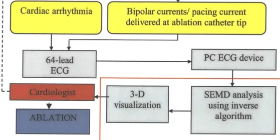
3.1 Overall RFA system design

--- --- 1

Cardiac arrhythmia

Bipolar curren

delivered at ab

64-lead

ECG

L..

ts/ pacing current

lation catheter tip

Figure 3.1: RFA device flow chart

3.1.1 Locating the re-entrant circuit

The complete radio-frequency ablation device would be designed as shown in Figure 3.1.

Potentials recorded by the 64-lead body-surface ECG are transmitted to a laptop computer, which simultaneously displays the input in real-time and stores the data in memory. The user interface to the device allows the cardiologist to examine the ECG recordings and select the data segment of interest in the VT waveform. This is processed by the SEMD inverse algorithm software, which outputs the dipole parameters for every sample in the selected data segment. The dipoles are then displayed in a 3-dimensional graphical interface. The cardiologist can manipulate this

environment and individually view each dipole's parameters. The dipole that best represents the ablation site is then chosen based on various factors (see section 8).

J

PC ECG device

3-D

_{SEM analysis}

visualization

_{using inverse}

algorithm

3.1.2 Guiding the Ablation Catheter

Once the dipole that best represents the ablation site is chosen, the cardiologist must align the ablation catheter tip and the dipole. The implementation of the ablation catheter is beyond the scope of this project; however, I will mention two design possibilities that would allow the cardiologist to do this.

If bipolar currents are delivered from the tip of a specially-designed catheter, at a frequency above the range of blo-potentials (1 to 250Hz), this can be detected by the body-surface electrodes. Once the signal is band-pass filtered at the frequency of these bipolar currents, the same inverse algorithm can be used to calculate the location of the catheter-tip 'dipole'. If the catheter-tip and reentry-site dipoles are matched both in location and orientation, it is hoped that tissue inhomegenities and systematic error will have no effect on the accuracy of the match.

An alternative approach is to pace with the ablation catheter tip at the same cycle length as the tachycardia and record the resulting ECG potentials. By sampling the electrode potentials that occur within a few milliseconds of each pacing stimulus, and finding the inverse solution to these potentials, we can locate the dipole closest to the catheter tip (and hence the tip itself, if good endocardial contact is maintained). As with the bipolar current method, tissue inhomogeneities would theoretically have no effect since only relative distance between catheter tip and re-entry site is important.

This second approach has numerous advantages. Firstly, the ablation catheter need not be custom designed, since commercially available catheters have the ability to both pace and ablate.

Furthermore, if the VT is fast, electrical activity from the previous beat is still present when the next wave of depolarization leaves the reentry circuit. Since an SEMD is the vector sum of all cardiac excitation this could introduce significant error into the dipole approximation. However, if the catheter tip were used to pace at the same rate as the VT, the excitation overlap would theoretically be the same and the relative error between the cardiac and catheter dipole approximations would be zero.

Lastly, the pacing option is more financially viable. Most commercially available ECG systems have a frequency cutoff around 250 Hz. If the bipolar current method were used, the bandwidth of

the ECG device would need to extend to at least 500 Hz to prevent bio-potential interference with the catheter-tip signal. High-bandwidth systems do exist, however they are far more expensive.

3.2 Biomedical Safety Considerations

Commercially available medical devices must conform to several safety guidelines, most importantly AAMI EC 11, IEC60 1-1, IEC601 -1-1, IEC601-1-2 and IEC601-2-25. These

guidelines relate mainly to hardware, and impose maximum values on lead leakage, ground-lead resistance, etc. However, some are applicable to the current software design project.

Electric shock is a major hazard in the medical environment. The patient is often connected to several monitoring devices simultaneously; if one of these develops an electric fault and the lowest-impedance connection to ground exists though the patient, he/she will be exposed to potentially lethal currents. If the ECG device develops a fault or provides this connection to ground, the position of the electrodes directly above the heart increases the risk of death. A current of only 75 to 400 mA in this region will cause ventricular defibrillation, while 1- 6 amps will cause a sustained myocardial contraction.

To provide patient isolation from the mains source, the software should be run on a battery-powered laptop. Secondly, to isolate the patient from ground, it is vital that the electrode connections to the ECG device have an input impedance of greater than 100 MOhm at

frequencies around 60 Hz. Also, since a defibrillator may need to be used if the patient develops a dangerous tachycardia, the ECG device should be protected to 4kV (360 Joules). This level of isolation can be provided if an isolation amplifier is used to filter and amplify the electrode signals, and these are streamed in real-time to the laptop-based ECG system via a fiber-optic cable or remote connection.

3.3 Choice of Operating System and Software

Safety considerations also affect the choice of operating system (OS). The OS must be able to perform in real-time, in a critical-care environment where loss of data due to a 'crash' could

are a significant advantage. One such operating system, the QNX OS, is currently used in several critical-care medical applications.

However, since this project was aimed more at 'proof of concept' than commercial-viability, it was decided to implement the system in Windows 2000/ME/XP in spite of its poor reputation for fault tolerance. Unlike UNIX, Windows has a physician-friendly interface. The Mac OS is also a possibility, although there are many more commercially available platforms that can support a Windows environment.

4.

The Graphical User Interface

4.1 User Interface Structure

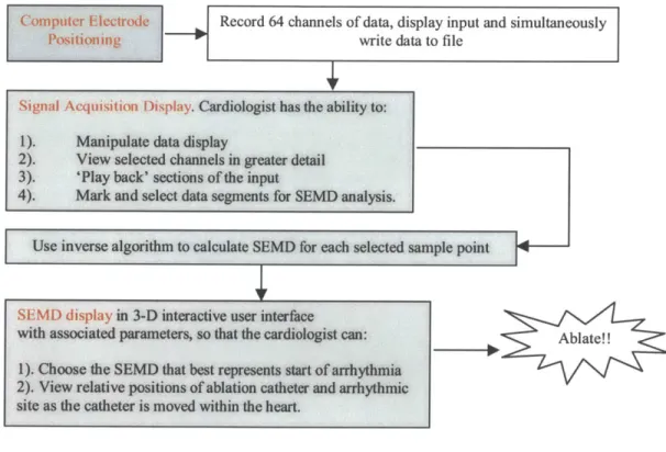
The flowchart in Figure 4.1 shows the broad structure of the user interface. For each step, a list of specifications was compiled and approved as described in this section.

Computer Electrode Record 64 channels of data, display input and simultaneously

Positioning write data to file

Signal Acquisition Display. Cardiologist has the ability to: 1). Manipulate data display

2). View selected channels in greater detail 3). 'Play back' sections of the input

4). Mark and select data segments for SEMD analysis.

Use inverse algorithm to calculate SEMD for each selected sample point

SEMD display in 3-D interactive user interface

with associated parameters, so that the cardiologist can: _{Ab ate!!} 1). Choose the SEMD that best represents start of arrhythmia

2). View relative positions

of

catheter

Figure 4.1: Flow Chart for User Interface

4.2 User Interface Specifications

The user-visible software consists of three graphical interfaces displayed in three different windows. All three windows may be displayed simultaneously, although the operator has the option of minimizing windows or moving them to alternative desktops.

I. Computer Electrode Positioning

The cardiologist must place the electrodes in the position assumed by the inverse dipole algorithm. The first graphical interface should permit the operator to view electrode position information and input patient information:

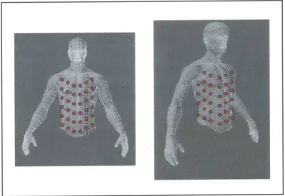
" _{Operator can select and display the appropriate torso model, with pre-defined electrode} positions. This option will help the operator properly align the patient electrodes with the torso model electrodes.

" The torso is presented as a 3D-wireframe model.

II. Data Acquisition display

Once the cardiologist has entered the patient data and correctly positioned the electrodes, the computer will begin recording data. By default, signals are displayed in real-time. Two types of

signals are displayed:

1. Standard ECG signals from catheters and body surface leads to use as part of the standard mapping protocol.

2. The individual electrode signals, to verify the quality of the electrode connection

After recording has finished, the operator is able to manually scroll backwards in time through the signals, or view the data as a 'movie'. 10 minutes of data should be accessible in RAM, and the remainder will be stored on the disk. The signal acquisition interface should have the following capabilities:

- Operator is able to manually adjust the display gain for individual channels - Operator is able to mark intervals between events with the mouse

- Operator is able to move the positions of individual channel displays on the screen to allow him/her to organize signals in a manner relevant to the catheter's position - Operator is able to select (and print out) a data segment for SEMD analysis

This data segment is passed to the inverse algorithm. The analysis is not done in real time. The SEMD parameters are calculated for each sample in the chosen segment and are then displayed.

III. Single Equivalent Moving Dipole (SEMD) display

There are two phases of operation. Initially, only the sequence of SEMDs related to cardiac excitation is displayed. Once the re-entrant dipole has been chosen and the ablation catheter inserted, the SEMD related to the catheter tip must be displayed also. In both cases, an individual dipole is represented by a three-dimensional ellipsoid (dipole ellipsoid), in conjunction with a dipole vector.

Individual SEMDs are displayed as follows:

- The position of the dipole ellipsoid center (and the start of the dipole vector) is the 3-dimensional location of the dipole.

" The dimensions of the dipole ellipsoid reflect the three-dimensional positional uncertainty of the dipole - a large diameter ellipsoid is poorly localized, while a small ellipsoid is highly localized.

* _{The color of the dipole ellipsoid indicates the magnitude of the dipole, using a two-color} sliding scale - red indicates large magnitude, blue is small magnitude.

" The orientation of the dipole vector reflects the orientation of the dipole

" _{The length of the dipole vector is constant. The ellipsoid is semi-transparent, so that the} dipole vector can be seen even if the dipole is poorly localized.

All dipoles from the data segment selected in the "Signal Acquisition" interface are initially presented in a 3-D rotatable display that demonstrates the trajectory of the cardiac dipole over that period.

" _{The data segment is presented as an 'arc' of colored dots, each dot indicating the} estimated spatial location of the dipole at that instant. Each dot is color-coded corresponding to the magnitude of the dipole as above (red is strong, blue is weak). " The cardiologist can step through this trajectory using a button on the interface. Each

" _{Parameters of the selected dipole are shown numerically on the side of the display.} - _{An ECG signal from a standard surface lead over the selected data segment is displayed.}

The time of the currently selected dipole is marked.

" _{The operator has the option of displaying the surrounding torso model selected during the} "Computer Electrode Positioning" phase. (This is only of physiologic use if the correct dimensions of the patient's heart are known. A CT scan of the patient's torso could generate a 3-D image of the heart, which would then be used by this program.)

" _{The operator can "zoom in" on a section of the trajectory to view dipoles more closely,} and return to the normal field of view.

The cardiologist will use the dipole trajectory and ellipsoid/vector display to determine the dipole that best represents the arrhythmic origin (for further discussion, see Section 8). This dipole is then selected and 'saved'.

The second stage of analysis involves the superposition of a "real time" display of the catheter tip with the single cardiac dipole selected above. The update rate of the display may only be once every few seconds (decided by the time required to calculate the catheter dipole parameters), but this should be sufficient since the catheter is moved slowly. The catheter tip dipole is displayed as a small dipole ball/vector.

4.3 Choice of Programming Environment

There were several important requirements concerning software environment:

" Must provide excellent data acquisition support, and wide compatibility with commercially available DAQ devices.

* Must have good graphical capabilities, in 3-D and in real-time.

- Must handle complex numerical calculations, and be able to handle large data matrices. - Must be programmatically able to provide a simple user interface for the physician.

LabVIEW (National Instruments) interfaced with Matlab (Mathworks) suits this purpose. LabVIEW is a graphical programming language that is perfectly suited to DAQ system user-interface design. Although numerical computation and 3-D visualization are poorly supported, it

is easily interfaced with Matlab, a language specifically designed to handle large matrices and mathematical equations. Matlab also has excellent 3-D image rendering capabilities.

Consequently, the Computer Electrode Positioning and Data Acquisition displays are implemented with LabVIEW. Matlab is then used to calculate the dipole parameters for the selected data segment and display these in a 3-D graphical user interface.

4.4 Data Sources

Since the goal of this project was to implement only the software component of the RFA device, pre-collected data was used to test the software. This data was obtained from several sources.

60-channel swine ventricular pacing data was pre-recorded at a sample-rate of 500 Hz by Dr. Antonis Armoundas, and saved as a series of '.d' files.

63-channel BSPM data, recorded at 250 Hz, was kindly donated by the research group of Dr. Didier Kiug from the Sacre-Coeur Hospital in Montreal. This data is single-beat, slow ventricular tachycardia data, recorded in a series of TIMI (Thrombolysis in Myocardial Infarction) studies. The data is saved in ASCII '.asc' format.

Lastly, to test signal-parameter estimation techniques (see Section 6), single-channel ventricular tachycardia and sinus rhythm data was obtained from the MIT-BIH Arrhythmia Database and the Creighton University Ventricular Tachyarrhythmia Database, both available through Physionet. These sources provided examples of signals with different rates and morphologies of VT, excessive baseline wander, and high-frequency noise. This data was recorded at a sample rate of 250 Hz, and saved in text '.txt' format.

5.

Signal Acquisition and Display

5.1 Patient Information Entry

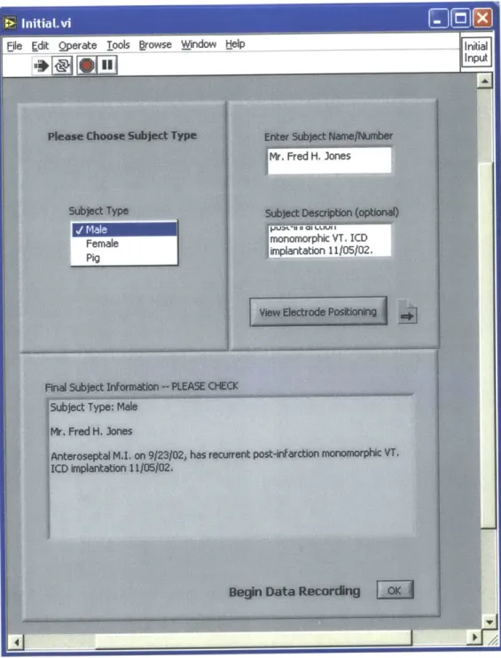
The initial display shown in Figure 8 allows the cardiologist to view the correct electrode positioning and enter pertinent patient information. The cardiologist first selects the patient's sex/type (male, female, or pig for research purposes) from the pulldown menu. The program uses this information to decide which wireframe model to display when the cardiologist clicks the button "View Electrode Positioning". Figure 5.1 shows the male BSPM electrode configuration.

Figure 5.1: Male Electrode Positioning Wireframe Torso Model

As shown in Figure 5.2, patient data entered in the two upper text boxes appears, along with the patient type, in the text box labeled "Final Subject Information". Once the cardiologist has finalized and checked the patient's information, and has positioned the electrodes as indicated by the wireframe model, he/she presses the button marked "OK" to begin data acquisition.

Figure 5.2: Patient Data Entry entry

-5.2 The Data Acquisition Interface

5.2.1 Signal Acquisition and Real-Time Display

The cardiologist is initially presented with a prompt to enter the name of the file in which the data should be stored, the number of electrodes that are being used and the sampling frequency (see Figure 5.3). After he/she clicks OK, the device begins recording to the specified file name. A program to interface with the ECG device has not been developed as part of this project, since its

design is dependent upon the final hardware chosen; also, it is often provided with commercially available devices. However, LabVIEW has excellent data acquisition capabilities therefore the design of such a program in the future would not be complicated.

*Soho"L.j d 12 LeU.& 13-24 2W [ U.W 37a-" U~

Figure 5.3: User prompt and initial screen before recording begins.

32 I

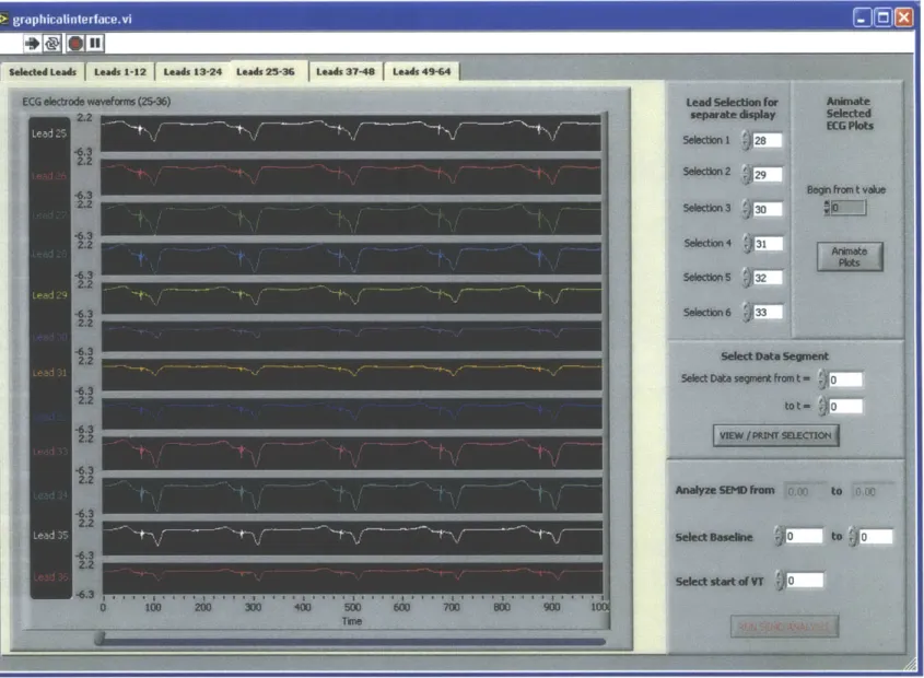
Signal data from all 64 channels is simultaneously written to memory and displayed. Since pre-recorded data is used in this project, scrolling the data across the display as it is read from the stored file mimics this process. As shown in Figure 5.4, the data is displayed in a series of tabbed pages; this arrangement works best for simultaneously displaying many sets of high-resolution data in a manageable way.

While recording, the data is displayed in real-time on tabbed-pages 2 through 6, divided according to the heading at the top of the page (e.g. 'Leads 1-12'). The limits of the Y-axes (in mV) on each page are adapted to the current data set, and are coupled to the maximum and minimum electrode voltage displayed on that page. The markings on the X-axes indicate the sample number. The program also dynamically sets the X-axis limits, so that two seconds of data are always displayed on the screen. For instance, for a sampling frequency of 250 Hz, 500 consecutive samples can be seen on the screen at a time. For ease of use, the signal legend and the signal itself are color-coded to match.

This tabbed display system allows the software to be easily extended if additional input channels are required. The inverse problem estimation improves with the number of inputs (the chi-square value of the estimated dipole decreases with addition of low-noise channels). Therefore, ease of extension will be a valuable feature when testing the completed ablation device.

5.2.2 Selecting a data segment

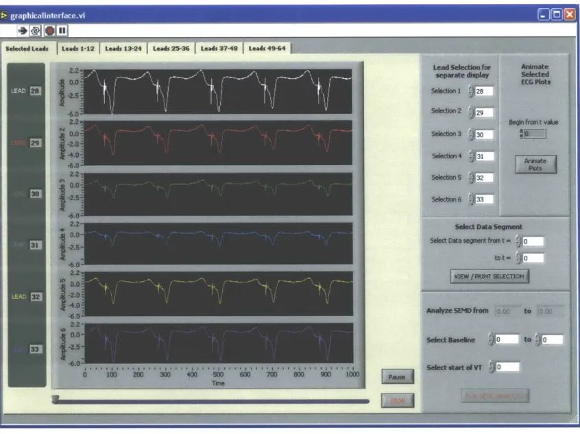
Once the data has finished recording, the user can scroll through the data using the scroll bars at the bottom of each page. The first tabbed page is used to display signals selected by the user that he/she would like to view at a higher display gain; for instance those with important

characteristics, or that have a low signal-to-noise ratio. This page is initialized to display the strongest signals out of the 64, which are invariably found in electrodes towards the middle of the torso. Using the digital controls in the top right panel of the interface, the user can change the selection and order of the channels as required (see Figure 5.5). The number of each selected channel is displayed next to its graph, and the scroll bar at the bottom can be used to scroll backwards and forwards in time.

Seleded Leads Leeds 1-12 Leads 13241 Leads 25-36 1 Leads 37-49 1 Leads 49-64

Figure 5.5: Display of selected leads i

The user can also view these signals as a movie. This is a useful feature if the cardiologist needs to inspect long data segments, since the signals will scroll automatically until paused. To do this, the cardiologist enters the time at which he/she wishes to begin the animation, and clicks on the

'Animate Plots' button on the right. The Animation Display is shown in Figure 5.6.

Figure 5.6: Animation of selected leads

The signals are displayed with their electrode number and scroll from left to right at a speed determined by the setting of the 'Animation Speed' dial. Control of the scroll speed is useful if, for instance, the patient is defibrillated after a period of tachycardia and the VT is then re-induced several minutes later; the cardiologist can scan quickly through the intervening period of sinus

By scrolling manually and using the animation feature the cardiologist will identify an arrhythmic beat, or a segment whose characteristics require closer examination. To view this section of the data more closely, print it, or to select a segment for SEMD analysis, the cardiologist enters the data range of interest into the text boxes in the panel marked 'Select Data Segment'. Clicking the button 'View/Print Segment' then opens up a new window displaying only the range of interest, as shown in Figure 5.7.

The signals shown in Figure 5.7 are from pre-recorded swine paced data. The features seen include the tail-end of the T-wave from the last beat (until approximately t = 1862), a pacing spike artifact (at t = 1876), and the QRS complex due to the pacing stimulus (starting at around t = 1895). We wish to image the dipole during, and especially at the beginning of, the QRS complex. Earliest activation of the ventricle is associated with a downward-turn of the lead potentials. Also, after the peak of the QRS the depolarization wavefront is too diffuse for its dipole representation to have any physical meaning. Therefore we choose the limits of SEMD analysis just before and just after the down-turn and peak of the QRS respectively.

To delineate the desired data range, the cardiologist first presses the button marked 'Display Cursors'. Two cursors appear whose numerical values are displayed in the text boxes marked 'Cursor 1' and 'Cursor 2'. To print the window, the cardiologist clicks the 'Print Display' button. To select the range demarcated by the two cursors for SEMD analysis the user presses 'Final Values Chosen'. This returns the user to the main display and passes the cursor values to the "Analyze SEMD" panel on the lower-right, where they are displayed in the text boxes. If the user did not select a data segment in the View/Print display, these boxes are inactive and appear blank (as in Figure 5.5). When the values shown are final, the cardiologist clicks the button "Run

SEMD Analysis" to calculate dipole parameters for all samples within the data range (see Figure 5.8).

SWx

I _Ix

0

6.

Signal Parameter and Dipole Estimation

6.1 Matlab Program Structure for Dipole Parameter Calculation

pace or VT. m

PaceProgram.m

Finds noise and baseline value

openSEMD.m

Open data, electrode _{isoelectric segment), and}

locations _{determines channels with good}

A

\V _in the channel, and the ratio of

Data paced or hr detect.m the noise to the height of the

VT? nace QRS complex)

VT VTprogram.m

Finds the noise value for each channel using the algorithm described below. Removes high-noise channels and those Determine channel l -- hr detect.m with a large noise-to-QRS ratio. baseline values. Call

inverse algnew.m*

with each sample's High-quality channels and noise values

baseline-corrected H

electrode voltages. moment.m

Output dipole location and orientation showspheres.m Displays dipole trajectory Call posUnc.m to newsemd.m

calculate Plot all dipoles and their imbed animation.m

positional parameters in 3-D gui. Displays individual

uncertainty of Idipole _parameters

each dipole

Using LabView's built-in Matlab Script Box, the values and data range specified by the user in the Data Acquisition Interface are passed to the programpaceorVT.m (see Appendix). This initiates the cascade of programs shown in Figure 6.1 that first calculate and then display the dipoles for each sample in the selected data segment. All Matlab programs have been included in the Appendix. Tamara Williams, a PhD candidate in Electrical Engineering at MIT, implemented the basic inverse algorithm as part of her thesis work (in Figure 6.1, these programs are indicated by an asterisk). Her program code is included in the Appendix with her permission.

6.2 Signal Parameter Estimation

6.2.1 Baseline Estimation

Baseline drift in an ECG lead is usually caused by respiration or movement of the subject. [36] The severity of baseline wander is different in each lead, and if two measurements are made far apart in time each lead's baseline may have changed significantly. Therefore baseline drift can significantly alter the dipole parameters found by the inverse algorithm. This is an important problem to consider if we are to match the catheter tip and reentrant circuit. Only by accurately baseline-correcting the lead values in the calculation of both dipoles will the inverse algorithm calculate the same dipole parameters.

If the baseline is assumed to be continuously changing its estimation is an inherently ill-posed problem, since 64 measurements are made while 6 dipole parameters plus 64 baselines must be found. There will always be six more variables than equations describing them; therefore it is impossible to devise an algorithm that will accurately estimate all parameters. If the baseline is assumed to be constant over a short time period, the problem becomes solvable. However, algorithms estimating this constant baseline by minimizing chi-square or RNMSE over any time period failed to find the correct value for data in which the baseline was known. Therefore, two approaches were devised, one for paced data in which the baseline can be observed empirically from particular time segments (see below), and another for VT data in which a signal-processing method must be employed.

e Paced Data

The ECG tracing above is taken from paced data and clearly shows the isoelectric period prior to the pacing spike. The T-wave has finished, the heart is repolarized, and cardiac electrical activity is essentially zero. If there were no baseline offset, the potential during this time segment would be zero. Therefore, the DC value of the signal during the isoelectric period is an excellent approximation of the current baseline. By calculating local gradients, the algorithm (a subsection

of Paceprogram.m) finds the most recent isoelectric period before the selected data segment. The

mean isoelectric signal value in each lead is then calculated. The baseline is assumed to remain approximately constant over the timescale of a beat.

- VT data

The isoelectric segment does not exist during ventricular tachycardia, since the next

depolarization begins before electrical activity from the prior beat has dissipated. Several signal-filtering approaches have been described to detect baseline. Morphological signal-filtering, a technique based on set operations, appears to be very effective in sinus rhythm [37] while wavelet

transforms are highly suited to identifying regular patterns within a signal and therefore removing baseline wander [38]. Adaptive signal filtering has also been employed. The American Heart

Association (AHA) recommends a cutoff frequency of 0.67 Hz for detecting DC and slowly-may

-Filtering the cardiac signal to detect baseline wander

A 4h-order lowpass Butterworth filter is a good choice for baseline detection, since its maximally flat passband will ensure minimal distortion of the baseline signal. However, this filter has a slow decay, therefore the signal may be distorted if the cutoff frequency is not sufficiently low. [40] The inbuilt Matlab functionfiltfilt.m will use pre-defined 4*-order Butterworth filter parameters to filter in both the forward and reverse directions, causing zero phase distortion and producing an 8W order roll-off.

To determine the appropriate cutoff frequency for baseline detection, the power spectra of several single-channel VT ECG signals with significant baseline wander were plotted. As shown in Figure 6.2, the power spectra characteristically show two low-frequency 'spikes'. The higher-frequency spike corresponds to the heart rate. The lower spike (below 1.5Hz) is due to baseline wander. For this data set, a cutoff frequency around 1.5Hz will capture the baseline frequency components.

Figure 6.2: Power Spectrum of

VT

0.5