HAL Id: hal-00304754
https://hal.archives-ouvertes.fr/hal-00304754
Submitted on 1 Jan 2003HAL is a multi-disciplinary open access archive for the deposit and dissemination of sci-entific research documents, whether they are pub-lished or not. The documents may come from teaching and research institutions in France or abroad, or from public or private research centers.
L’archive ouverte pluridisciplinaire HAL, est destinée au dépôt et à la diffusion de documents scientifiques de niveau recherche, publiés ou non, émanant des établissements d’enseignement et de recherche français ou étrangers, des laboratoires publics ou privés.
a casestudy from the Pevensey Levels, UK
R. B. Bradford, M. C. Acreman
To cite this version:
R. B. Bradford, M. C. Acreman. Applying MODFLOW to wet grassland in-field habitats: a cases-tudy from the Pevensey Levels, UK. Hydrology and Earth System Sciences Discussions, European Geosciences Union, 2003, 7 (1), pp.43-55. �hal-00304754�
Applying MODFLOW to wet grassland in-field habitats: a case
study from the Pevensey Levels, UK
R.B. Bradford and M.C. Acreman
Centre for Ecology and Hydrology, Wallingford, OX10 8BB, UK Email for corresponding author: rbb@ceh.ac.uk
Abstract
Historical drainage improvements have created complex hydrological regimes in many low-lying, wet coastal grassland areas. The manipulation of ditch water levels is a common management technique to maintain important in-stream and in-field habitats in such areas. However, in wet grasslands with low soil conductivities the water table in the centre of each field is not closely coupled to variations in ditch stage. Consequently rainfall and evaporation have a greater influence on the depth to water table and water table fluctuations within each field. In-field micro-topographic variations also lead to subtle variations in the hydrological regime and depth to water table that create a mosaic of different wetness conditions and habitats. The depth, duration, timing and frequency of flooding from accumulated rainfall, surface water and standing groundwater also influence the availability of suitable in-field habitats. Land drainage models are often used for studies of wet grasslands, but tend to be more complex and require more field variables than saturated zone models. This paper applies a 3D groundwater flow model, MODFLOW, to simulate groundwater levels within a single field in a wet coastal grassland underlain by a low permeability sequence and located in the central part of Pevensey Levels, Sussex, UK. At this scale, the influence of vertical leakage and regional groundwater flow within the deeper, more permeable part of the sequence is likely to be small. Whilst available data were not sufficient to attempt a full calibration, it was found that the sequence could be represented as a single, unconfined sequence having uniform hydraulic properties. The model also confirmed that evaporation and rainfall are the dominant components of the water balance. Provided certain information requirements are met, a distributed groundwater model, such as MODFLOW, can benefit situations where greater hydrological detail in space and time is required to represent complex and subtle changes influencing the in-field habitats in wet grasslands with low permeability soils.
Key words: wetlands, hydrology, groundwater, MODFLOW
Introduction
‘Lowland wet grasslands’ is a generic term that includes river floodplains and coastal grazing pastures, such as the Pevensey Levels in East Sussex, UK. These are characterised by periodic inundation and/or a high water table and have a flat topography dissected by a dense network of drainage channels. They provide important habitats for plants, invertebrates and birds (Joyce and Wade, 1998) and are well represented in England, having a total area of about 200 km2 (Jefferson and Grice, 1998).
The management and maintenance of lowland wet grasslands relies mainly on the control of ditch water levels, but this is often hampered by the complexity of the hydrological regime, the density of the drainage network and shared responsibilities for the operation of the ditch control structures. In the UK, Water Level Management
Plans (MAFF, 1994), agreed between the various stakeholders, are employed to meet objectives ranging from intensive agricultural production to wildlife conservation. The Wildlife Enhancement Scheme (WES) also provides subsidies to farmers to manage their land in a way that encourages wildlife. This scheme includes maintaining ditch water levels at prescribed levels depending on the time of year.
However, the manipulation of ditch water levels has less influence on the water table elevation in wet grassland areas with low soil permeability such as the Pevensey Levels. During the winter months, the water table in the centre of a field is higher than the water level in the surrounding ditches but lower during the summer months. The fields have a ‘saucer-shaped’ topography due to excavated ditch material being deposited at the field boundaries so that the water
table is closer to ground level in the centre of the field than adjacent to the ditches. Small-scale topographic variations ranging from about 0.2 to 0.3 m within each field also determine the depth to water table and consequently evaporation rates, recharge and the extent of groundwater flooding at any particular location and time. This produces variations in the water regime within the field and hence a mosaic of different habitats for plants, insects and birdlife (RSPB, 1997).
The extent, depth, frequency, timing and duration of flooding within the fields during the winter and spring are important to provide roosting, feeding and breeding sites for a wide variety of bird species. The winter flooding results from a variable combination of surface water overflow from the ditches, standing groundwater when the water table intersects the ground surface and accumulated rainfall on the saturated surface.
In-field habitats in wet grasslands with low permeability soils are affected by complex and subtle changes affecting the water regime that are not easily taken into account in existing management models. Most management studies at the field scale are undertaken with 2D models based on land drainage and soil physics theory to simulate the water table response to hydro-meteorological variables. Examples include DRAINMOD (Skaggs, 1980), SWATRE (Belmans
et al., 1983), FDRAIN (Armstrong et al., 1980; Armstrong,
1993) and DITCH (Armstrong and Rose, 1999; see also Youngs et al., 1989, 1991).
Physically-based, process orientated, spatially distributed models, such as MIKE-SHE (e.g. Al-Khudhairy et al., 1999), have seldom been applied to the study of low wetlands as these are rather complex to operate and require a level of data that is seldom available in such areas. Groundwater flow models can also represent many of the features influencing the in-field water regime, including anisotropy and heterogeneity in hydraulic properties. They are more commonly applied to wetlands where groundwater is an important component of the hydrological regime (e.g. Leemhuis and Al-Khudhairy, 2001; Gilvear et al., 1997).
This paper examines the general application of a groundwater flow model, MODFLOW (McDonald and Harburgh, 1988), to in-field water table variations using data available from the Pevensey Levels. However, the data necessary to develop a fully validated groundwater flow model for water management purposes are not available from this site.
Modelling approaches
The study of in-field situations can require complex three-dimensional analyses to derive time-varying water table
elevations over an irregular shaped field bounded by partially-penetrating drains as line sinks (or line sources in summer) with variable stage and in hydraulic continuity with the underlying strata. They may also need to accommodate spatial and depth variations in soil hydraulic conductivity, porosity and specific yield and spatially varying evapotranspiration.
A water balance approach may be appropriate for simple situations, such as that adopted by the DRAIN model (Armstrong and Rose, 1999):
ht = ht-1 + (R-Et-Qd)/f
where ht is the water elevation at time t, R is rainfall, Et is evapotranspiration, Qd is the flux through the drainage systems and f is the soil porosity. Depth variations in hydraulic conductivity can be taken into account in this model. A water balance approach to predict ditch stage was also used as the basis for a physically-based model (PINHEAD) developed by Gasca-Tucker and Acreman (1999) and applied to a hydrologically-discrete ditch system near the centre of the Pevensey Levels.
Models based on drainage theory have been developed to simulate the flux of water from the soil to bounding ditches to estimate the water table elevation within the field. These were developed originally for engineering purposes to predict the steady-state maximum water table elevation midway between fully-penetrating, parallel drains spaced distance 2D apart. Many of the features required for in-field habitat studies are taken into account in a numerical procedure based on land drainage and seepage theory by Youngs et al. (1989) to predict the water level change ∆H during a time interval ∆t at a given site surrounded by ditches containing water at a known height. This is based on the following equation:
∆H = {(K1-K0)/AmSD2(k(H0-b)2 – j(Hm-b)2) + K0/AmSDá(H
0á – i(iHm)á) – V/S}∆t (1)
where H0 and Hm are mean heights of the water table above
an impermeable base over the time interval, S is specific yield, D is the drain half-spacing, K1 and K0 are the hydraulic conductivities of the topsoil and subsoil respectively with the division between these at height b above the ditch base,
Am is a geometrical factor, V total flux due to rainfall and evaporation, and j and k take values of 1 or 0 depending on the respective heights of Hm and Ho to b. Non-steady-state water table fluctuations are considered as a succession of steady-states. Depth-dependent specific yield can be accommodated as well as heterogeneity in the hydraulic conductivity of the soil, which is a particular problem in
applying soil physics theory. Actual evaporation is assumed to be the potential evaporation as long as the soil is not limiting evaporation due to the depth to the water table. When this is not the case, evaporation from the water table under steady-state conditions is derived from Richards’ equation for which knowledge of the unsaturated zone hydraulic conductivity K(p) at a soil water pressure p is required.
Further development of this model to study in-field habitats was made by Youngs et al. (1991, see also Childs and Youngs, 1961), who describe a numerical procedure to model a 3D drainage situation to produce contour maps of water table elevation, h(x,y), over a field surrounded by water-filled ditches:
H(x,y) = [2E*Hp2 + H
o2(1 - 2E*)]1/2 (2)
where Hp is the mid-drain water table height that would occur if the field were drained by a parallel system of drains spaced 2D apart and E* = (Eo – E)/VD2, where E is the gradient of
the seepage potential and Eo is seepage potential (2E* is equal to A in Eqn. 1). Contours of E* show locations having the same seasonal range in water levels.
Soil physics based models have been applied successfully to a range of different low wetlands in UK, in particular to investigate drain spacing and stage controls in more permeable wetlands. These models usually require more field variables than saturated zone models and consequently are more complex. Some of the factors influencing in-field habitats in low permeability wetlands with irregularly shaped fields and partially penetrating ditch systems are also less easily accommodated in such models.
A key requirement for studying in-field habitats is often an adequate and reliable simulation of spatial and temporal variations in hydro-meteorological variables associated with topographic variability in order to produce time-series depth to water table maps, which in many situations can provide an indication of the soil water conditions at the soil surface. For example, evapotranspiration rates will vary across the field according to water table depth and vegetation type, cover, growth stage and rooting depths. Other subsurface components of the water balance may include vertical leakage to or from any deeper, more permeable strata and more regional groundwater flow towards major drains or the coast that are not taken into account in soil physics based models.
MODFLOW is a finite difference, 3D, time-varying groundwater flow model that has become the industry standard for many groundwater-related studies. The general form of the governing partial-differential equation describing groundwater flow under time-varying conditions
in a heterogeneous and anisotropic aquifer is:
(3) where x, y and z are Cartesian coordinates aligned along the major axes of hydraulic conductivity Kxx, Kyy and Kzz; h is the potentiometric head; W is the flux per unit volume representing sources/sinks; Ss is the specific storage; and t is time.
MODFLOW employs a block-centred approach and a modular structure consisting of a main program and a series of sub-routines grouped into packages. Each package includes specific features of a hydrological system, such as recharge or drains, and various methods to solve the linear equations (see Anderson and Woessner, 1992). A wide range of additional modules has been added since MODFLOW was developed originally (e.g. cell re-wetting or spatially variable anisotropy). A wetland module is available (Restrepo et al., 1998), although this was developed for swamp areas rather than grass wetlands. Commercial versions of MODFLOW provide a comprehensive suite of techniques to assist model design, to input data and analyse and present model output. The program code is freely available in the public domain, and commercial Window-based versions with pre- and post-processors are inexpensive. The model code employed for this study was Visual MODFLOW (version 2.72) developed by Waterloo Hydrogeologic and incorporating MODFLOW-96 (Harburgh and MacDonald, 1996).
Besides ease of use, the application of a groundwater model, such as MODFLOW, to in-field water regime studies has several potential benefits. For example, it can take account of spatial heterogeneities, vertical groundwater flow and any regional groundwater flow component. Whilst vertical leakage through clay sequences will occur at a low rate, and consequently will be a minor component at the field scale, the volume of leakage could be significant over the total area of a wetland. Irregular field boundaries and steep hydraulic gradients adjacent to a drain can be accommodated, although with a finite difference approach this may result in an excessive number of grid cells particularly with multiple layers. Recharge can be distributed areally and, although recharge is assumed to be added instantaneously to the saturated zone, this is not necessarily a disadvantage where the depth to water table is shallow even in low permeability sequences.
Evaporation from the soil is accommodated by the Evaporation Package in MODFLOW. A maximum evaporation rate is assigned to each cell when the water table equals an assigned head value (normally ground level)
y h Kyy y h Kxx x ∂ ∂ +∂ ∂ ∂ ∂ + ∂ ∂/ ( / ) / ( / ) t h Ss W z h Kzz z ∂ ∂ − = ∂ ∂ ∂ ∂/ ( / ) /
and ceases below a user-prescribed depth (extinction depth). The rate of evaporation is assumed to vary linearly between these two extremes, although the reduction in evaporation with depth is usually non-linear. Hence, the rate of evaporation and extinction depth can be varied in each cell with time, for example to accommodate different rooting depths associated with different vegetation distributions.
Another important feature of MODFLOW is the ability to represent a wide range of different drainage situations (drain, river or stream Packages), including variable stage, different drain depths, geometry or configurations, bed permeabilities and to accommodate situations when the water table falls below the bed of the channel. The hydraulic conductivity of the bed of field drains penetrating a clay sequence can be assumed to equal that of the sequence.
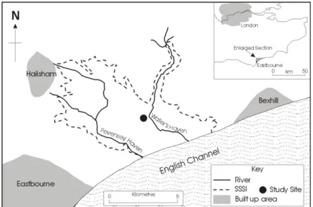
Study area
The Pevensey Levels are a wet coastal grassland situated between Eastbourne and Bexhill-on-Sea, East Sussex, on the south coast of England (Fig. 1). They cover an area of about 75 km2, have a mean elevation of 2 metres above
mean sea level (OD, Ordnance Datum) and are bounded by the low hills of Tunbridge Wells Sands to the north, by Wadhurst and Weald Clays to the east and west, and is separated from the English Channel to the south by a shingle ridge. The area is used mainly for grazing but is also a designated RAMSAR site (under the international convention on wetlands) and contains two National Nature Reserves. Important ecological features include invertebrates, such as the fen raft spider, and over-wintering and breeding bird populations. Jenman and Kitchen (1998)
and Gasca-Tucker (2002) provide detailed descriptions of the area.
The Levels are an alluvial floodplain that has been subject in the past to periodic marine inundation (Jennings and Smyth, 1985). This has produced a complex and variable lithostratigraphy with a complex basal geometry. The sequence broadly comprises a surface layer of clayey-silt up to 2 m thick, a discontinuous peat layer 0.6-1.8 m thick and fluvial clayey-silts 3-10 m thick, with intercalated fine to medium sands and silty sands representing buried channels, overlying Weald Clay (Phillips, 1995; Lake et al, 1987). The soils belong to the Newchurch and Wallasea series, which are generally slowly permeable and seasonally water logged (Jarvis et al., 1984).
The wetland has been reclaimed progressively and modified extensively by drainage improvements for agriculture and flood relief since the Middle Ages. This has created a complex hydrological regime. The present drainage network, which crosscuts a remnant drainage system, has a total length of 715 km with an average ditch density of 17.4 km km–2, of which 80% are minor ditches (field drains).
Eighteen pumps and numerous structures have been installed in the ditch network to control ditch levels. The network drains through major drains to the sea at Norman’s Bay and Pevensey Bay. However, the surface water inflow and outflow components are relatively small and the overall water balance is dominated by rainfall and evaporation (Acreman and José, 2000; Gasca-Tucker and Acreman, 1999).
The model study is focused on a National Nature Reserve (specifically Field 116) some 2.5 km2 in extent near the
centre of the Pevensey Levels where water level and other
monitoring data are available. This is an unimproved area of grassland dominated in the wetter parts by Agrostis spp and Juncus spp, which are important for migrating waterfowl.
The availability of the appropriate field data is often a constraint on applying models to wetland areas, and the Pevensey Levels are no exception. A monitoring network was established in the mid-1990s for three fields in the centre of the wetland and data of varying frequency and completeness are available between 1995 and 1998. The instrumentation in the vicinity of Field 116 comprises (see Fig. 4):
z a stage recorder on the main drain upstream of the study
site with daily readings from February 1995 to July 1998. The record is of good quality and essentially continuous.
z a Hydra Mk2, which measures evaporation by eddy correlation (Shuttleworth et al., 1988), and an Automatic Weather Station (AWS) providing daily actual (AE) and potential evaporation (PE), respectively. The AWS data are almost continuous from June 1996 to June 1998. Rather limited and intermittent data are available from the Hydra (14 days in September, 1996, 4 days during the summer 1997 and 31 days between June and September, 1998).
z a local meteorological station at Horse Eye some two
kilometres north-west of Field 116 with continuous
daily data on open water potential evaporation (Eo) and rainfall since 1970.
z a water level monitoring array of 10 dip wells (to 0.8–
1 m depth) and two piezometers (to 3.3 m depth) with data for 1995 to 1998. However, the continuity and number of readings are rather sparse due to difficult access in winter and drying-up of the dip wells during the summer. The configuration of the water table cannot be determined from the distribution of dipwells. Monthly MORECS (Meteorological Office Rainfall and Evaporation Calculation System, see Hough and Jones, 1997) data on actual and potential evaporation, rainfall and soil moisture deficits for 1961–1998 were also obtained for 40 × 40 km square 199 which includes the Pevensey Levels. These represent average values for the square, which also includes the higher ground bordering the Levels. The mean rainfall is 763 mm y-1, open water evaporation 774 mm y-1
and potential evaporation 655 mm y-1. The monitoring period
(1995-1998) was variable hydro-meteorologically. The summer of 1995 was particularly dry and 1996 had 95 mm less rainfall than the long-term average, whereas 1997 and 1998 had 130 and 145 mm, respectively, more rainfall than the long-term average.
Figure 2 shows the available estimates of evaporation for the period 1995 to 1998: daily open water evaporation at Horse Eye, potential evaporation based on the AWS and actual evaporation from the Hydra, together with monthly
0 1 2 3 4 5 6 7 8 9 10 01 /0 1/ 1 997 1/ 14 /9 7 1/ 2 7 /97 02/ 0 9/ 199 7 2/ 2 2 /97 03/ 0 7/ 1 9 9 7 3 /20/ 97 04/ 02 /1 9 9 7 4/ 15/ 97 4/ 2 8 /9 7 05/ 11 /199 7 5/ 24/ 97 06/ 0 6/ 199 7 6/ 1 9 /97 07/ 0 2/ 1 9 9 7 7 /15/ 97 7/ 2 8 /9 7 08/ 10 /1997 8/ 2 3 /9 7 09/ 05 /199 7 9/ 1 8 /9 7 10/ 0 1/ 199 7 10 /1 4/ 9 7 10/ 2 7/ 9 7 11 /0 9/ 1 997 11/ 22 /9 7 1 2 /0 5/ 1997 12/ 18 /9 7 12 /3 1/ 9 7 1/ 1 3 /9 8 1 /26/ 98 02 /0 8/ 1 998 2/ 21/ 98 03 /0 6/ 1 998 3/ 19 /9 8 0 4 /0 1/ 1998 4/ 14 /9 8 4/ 2 7 /98 05/ 1 0/ 1 9 9 8 5 /23/ 98 06/ 05 /1 9 9 8 6/ 18/ 98 07 /0 1/ 1 998 7/ 14/ 98 7/ 27/ 9 8 08/ 0 9/ 199 8 8/ 2 2 /98 E v a p or a ti o n ( m m )
Ho rse E ye ta nk Eo Auto m atic W e ath er S tation P en ma n P Et Hy dra A Et More cs A Et
Model representation
The model area is 400 × 400 m. The main surface features are shown in Fig. 4 and a transect showing the position of the water table in relation to the ditch level at high, average and low conditions, is shown in Fig. 5. During the winter, the water table within the field is higher than the stage in the ditch and lower during the summer but remains in hydraulic continuity with the ditches throughout. The model is orientated NW-SE parallel to the dominant direction of the drainage system to reduce the number of grid cells. This is also the assumed direction of regional groundwater flow (based on the topographic slope because spatial water level data are not available to define the direction of groundwater flow). The initial head was assumed to be uniform across the model area as the topographic gradient is very low.
During the initial calibration of the model, it became apparent that the field drains act as hydraulic boundaries around each field. Consequently, each field forms a discrete hydraulic unit with its own water table configuration. There may, however, be a more regional piezometric surface associated with the deeper sequence of deposits. The actual model domain was, therefore, limited subsequently to a single field (Field 116) by introducing inactive cells in all cells outside the field.
The ditches surrounding the field are typically 1.5 m in depth (bed level 0.8 mOD) and 3 m wide. These were represented as stage-controlled, head boundaries. The water level recorder situated just north of Field 116 provided data
1 1.1 1.2 1.3 1.4 1.5 1.6 1.7 1.8 1.9 2 2.1 2.2 2.3 2.4 2.5 0 9 /0 2/ 19 95 09 /0 4 /19 9 5 0 9 /0 6/ 19 95 09 /0 8 /19 9 5 09 /1 0/ 1 9 9 5 09 /1 2 /19 9 5 0 9 /0 2/ 1 9 96 0 9 /0 4/ 1 9 96 09 /0 6/ 1 9 9 6 0 9 /0 8/ 1 9 96 09 /1 0/ 1 9 9 6 0 9 /1 2/ 1 9 96 0 9 /0 2 /19 97 0 9 /0 4/19 97 0 9 /0 6 /19 97 09 /0 8 /19 9 7 09 /1 0/ 19 97 09 /1 2 /19 9 7 09 /0 2 /19 9 8 09 /0 4/ 1 9 9 8 09 /0 6 /19 9 8 mO D F3 Ditch stage F3/P(C) F3/D7 G ro und lev el D 7: 2.21 3 m O D S im u lation pe riod
Fig. 3. Water level and ditch stage hydrographs, 1995-1998
actual evapotranspiration based on MORECS. Evaporation data from the Hydra have been compared to estimates based on Penman-Monteith and Priestley-Taylor (Hall, pers. comm.). This indicated that most evaporation occurs when the wind direction is 240o, the prevailing wind direction, so
that evaporation rates within wet grasslands can exceed those that might be expected for well-watered grass. In addition, whilst the Priestley-Taylor method is adequate for monthly estimates of evaporation, the Penman-Monteith method provides better estimates of daily evaporation from wet grasslands.
Figure 3 shows water level variations during 1995 to 1998 in a dip well (D7) and nearby piezometer (PC) located near the centre of Field 116, together with ditch stage measured at the water level recorder. D7 is 1.11 m deep and situated 96 m from the nearest ditch whilst PC was installed to 2.5 m depth and is 110 m from the nearest ditch. The ditch stage is generally about 0.2 m lower than the water levels in both the dip well and piezometer during the winter and slightly higher during the summer. Water levels reach ground level during wet winters, such as in 1997/98 when water levels at D7 were about 0.1 m above ground level and would have produced groundwater flooding. There is some suggestion that water levels in the piezometers are higher than those in the dip wells, such as in 1995-96. This could suggest increasingly confined conditions with depth and, therefore, the possibility of vertical leakage of groundwater.
on stage variations within the ditches (see Fig. 3). The stage throughout the ditch system within the model domain was considered uniform at any one time. Ditch levels are one of the few known input variables, although groundwater level data were used for calibrating the model. As the ditches generally penetrate only the shallow clay layer (see Fig. 5), the permeability of the ditch bed sediments is considered to be the same as the surface clay layer.
The initial three-layered model represented the surface clay (Layer 1), the peat layer (Layer 2) and the underlying sediments (Layer 3). However, if required, heads within the individual parts of the sequence could be examined and the deeper sequence treated as semi-confined with a vertical groundwater leakage component. Each layer is assumed to be horizontal, homogeneous and isotropic.
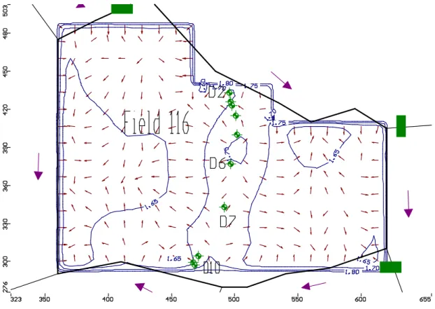
A grid mesh size of 10 m was used, although this was reduced to 2.5 m adjacent to the field ditches to accommodate steeper hydraulic gradients at these locations. The total number of grid cells was 10800 for the three layers and model area. The model grid is shown in Fig. 6. The surface topography was derived from a survey carried out over the area, although this did not extend to the northern part of the model area.
Fig. 4. General features of model area. Note that topography is based on DTM in mOD and did not include the northern part of the model area. The dip well array across the model domain (Field 116) is also shown.
The mean thickness of the surface clay layer (L1) is 1.7 m. Values of hydraulic conductivity (K) of the clay layer are available from pumping tests undertaken on the dip wells (Gasca-Tucker, 2003). These range from 0.172 to 0.002 m d–1 with a mean of 0.058 m d–1, similar to a typical K of
0.024 md-1 for alluvial clays reported by Armstrong (1993).
The mean K from the pumping tests was adopted for the surface clay layer. In general, soils with K values less than 0.1 m d–1 are classified as ‘slowly permeable’ (Jarvis et al.,
1984).
The thickness of the peat layer (L2) is 0.5 m based on the limited information from the piezometers. Peat deposits are often anisotropic due to compaction and secondary permeability features and often show a correspondingly wide range in hydraulic conductivity. However, a K value of 1 m d-1 is considered typical of peat soils (Armstrong, 1993)
and this was adopted initially for the peat layer. The horizontal permeability of peat deposits is often much greater than the vertical permeability and, as the peat layer is discontinuous and thin, it would have a very low transmissivity.
There is no information available on the hydraulic characteristics of the deeper layer (L3) which forms the bulk
0 0.5 1 1.5 2 2.5 245 250 255. 5 265 267 269 274. 5 280 285 290 295 300 305 310 317. 5 330 350 367. 5 377 382. 5 389 396 402. 5 407. 5 412. 5 417. 5 422. 5 427. 5 432. 5 437. 5 439. 5 442. 5 m od e l co o rd in a te s (m ) E lev at io n ( m OD )
ground level (m O.D) H m ax (m O.D), w ater table Hm in (m O .D), water table Hm ean (m O.D), water table bottom of clay lay er Hm ax (m O .D), ditch level Hm in (m O .D), ditch level Hm ean (m O.D), ditch level
NW S E
Peat Clay
Fig. 5. Transect across Field 116 showing high, mean and low water levels in relation to ditch stage. Note that in some cases, the minimum water level shown is the bottom of a dip well (i.e. dry) and the actual water level will be below this level. Base of clay is shown for
representative elevation. Ground level based on MODFLOW interpolation of topographic survey.
of the sequence. It was assumed to be 10 m thick and to consist of silty sands. Such deposits are likely to have K values in the range of 0.1 to 10 md–1 (Anderson and
Woessner, 1992) giving a transmissivity of at least an order of magnitude greater than the surface clays. Regional groundwater flow towards the coast is likely to take place within this layer.
Storativity values for each layer were based on typical values given in the literature. There are insufficient data to estimate such values from the water table response to rainfall events (Gilman, 1994). Specific yield (Sy) values for alluvial deposits are likely to range from 1 to 10% (mean 6%) for clays and 10 to 30% for silty sands. Specific storage (Ss) values of 10–3 to 10–2 m–1 would be representative of the
clay and 10–5 to 10–3 m–1 of the silty sand.
In MODFLOW, recharge is normally estimated and entered as input values into the Recharge Package. The water table remains close to the ground surface throughout the year (minimum water levels ranged from 0.7 to 1.2 mbgl during 1995 to 1998) and is subject to evaporative losses. For the initial calibration, rainfall data from the Horse Eye meteorological station were used as ‘recharge’ input values and applied uniformly over the model domain as 10-day mean daily values. The Evaporation Package of MODFLOW was then used to simulate evaporative losses from shallow groundwater and soils. The initial input values were based on MORECS actual evaporation data and applied uniformly over the model with an extinction depth of 1.0 m. In this way, the model itself was used to calculate ‘net recharge’. Whilst representing the general pattern, the MORECS monthly values may underestimate the real evaporation and its variability (see Fig. 2).
Model calibration and discussion
The model was run in time-varying mode with a time-step of 10 days and an initial head of 1.8 mOD (the mean of available head data for a well situated in the middle of the array of wells) applied to all three layers. The period January 1997 to August 1998 (577 days) was chosen for the calibration as this period has the most detailed water level data. The water table configuration across the field is not known and calibration was based mainly on water level hydrographs for wells in the centre of the field (D6) and close to the ditches (D2, north; D10, south). The results of the model calibration results were expressed as water table contour maps and directions of groundwater movement together with mass water balances for the model domain and zonal water budgets for flow to the ditches around the field at selected times.
The initial calibration runs with the hydraulic properties
assigned to each layer matched the observed water levels for the first 300 days but significantly overestimated water levels during the following winter period. A constant K, equal to that of Layer 1 (0.058 m d–1), applied to all three
layers produced a similar result but raised water levels still further. Subsequently, the Sy value for Layer 1 (5%) was applied to the other two layers to simulate a uniform sequence with water table conditions. This produced a reasonable fit to the general temporal pattern in terms of elevation and range of fluctuations, except during the initial period when the fluctuation is rather less than that observed. A higher initial head of 2.1 mOD improved the fit for the first 90 days but still failed to reproduce the initial decline in observed water levels up to about 150 days. The overall fit could be improved by further optimisation of the Sy value, although this was not justified on the basis of the lack of information on this variable. However, sensitivity runs with Sy values of 2.5 and 10% indicated that the model is relatively insensitive to the Sy value. The model is also relatively insensitive to K due to the low permeability of the sequence. The thin peat layer also appears to have little influence.
The results of the calibration with uniform hydraulic properties are shown in Fig. 7 as hydrographs for the three wells. Water levels in all three wells are very similar, but D10 (adjacent to the southern ditch boundary) is slightly higher in summer and lower in winter than D2 (adjacent to the northern ditch boundary) and D4 has water levels intermediate between the other two wells. The cumulative mass balance at the end of the calibration period (t = 577 days) is given in Table 1. This demonstrates the importance of rainfall and evaporation in the water balance compared to the drainage ditches.
Water level contours and flow paths for low (t = 200 days) and high (t = 350 days) water level conditions are shown in Figs. 8 and 9, respectively. The pattern is similar for both times with flow moving towards the depressions within the field from the surrounding ditches. This seems to reflect the influence of evaporation and the extinction depth,
Table 1 Cumulative mass balance (m3) at t = 577 days
IN % of total OUT % of total
Storage 24784 33.6 26806 36.3
Recharge 47538 64.4 -
-River leakage 1507 2.0 1644 2.2
Evapotranspiration - - 45379 61.5
although the imposed boundary conditions do not accommodate deeper subsurface flow into or out of the model domain. The influence of the drainage ditches on groundwater levels extends only about 20 m from each ditch during high water level conditions (Fig. 9). Cross-sections show an upward movement of groundwater in summer and downward movement in winter with the water table higher than the ditch stage in winter and lower in the summer.
Recharge will not occur where and when the water table is at the ground surface. The monitoring wells are situated along slightly higher ground where the topography generally exceeds 2.3 mOD (maximum 2.7 mOD). Surface elevations across the rest of the field either side of this ridge range from about 2.1 to 2.2 mOD (see Fig. 4) but are still generally higher than the maximum ditch stage, which varies from 1.2 to 2.1 mOD (see Figs. 3 and 5). The water table exceeded 2.2 mOD (taken to be a representative field elevation) in Jan/Feb 1997 and Jan/Feb 1998 (t = 0 to 50 days and 370 to 430 days, respectively), although there is no information on the extent or depth of flooded areas or the water table configuration across the field. A model run with no recharge (rainfall) for these two periods had no apparent effect on water levels. This may be due in part to low evaporation losses during the winter months. However, the model water table contours simply equal the ground surface contours when the water table reaches ground level. Consequently,
the model’s water table contours do not represent reality when this situation occurs, as the configuration is not governed by the hydraulic properties. The equipotential contours shown in Fig. 9 indicate the height to which the piezometric surface might rise above ground level.
The Root Mean Square error (RMS) of the model calibration increases from 0.14 (mean error –0.123) at low water table conditions to 0.24 (mean error 0.22) at high water level conditions. However, a more accurate calibration was not justified due to the lack of spatial data on, for example, the local flow pattern, extinction depth or hydraulic properties with depth. Similarly, the variations in topography, water level and other parameters are small scale and would require more detail to develop a validated model of the accuracy required for management purposes.
Conclusions
An initial conceptualisation of the system was based on a semi-confined, three-layered sequence with differing hydraulic characteristics. During calibration, however, it was found that a reasonable match between model and observed time-series water level data could be achieved based on an unconfined, single layered model with a uniformly low permeability for a single field unit bounded by partially-penetrating, head-controlled ditches. Spatial data are
Fig. 7. Calibration against observed water level fluctuations, Jan 1997 to August 1998
1.4 1.5 1.6 1.7 1.8 1.9 2 2.1 2.2 2.3 2.4 2.5 2.6 2.7 2.8 0 5 0 1 00 1 50 2 00 2 50 3 00 3 50 4 00 4 50 50 0 55 0 Tim e ( da ys ) W a te r le v e l e le v a ti o n ( m O D )
D2 model D6 m odel D10 model
Fig. 8. Low (summer, t = 200 days) water table configuration (mOD) and directions of groundwater flow for model domain (Field 116). Water table contours are shown to 2 decimal places, topographic contours to one decimal place.
Fig. 9. High (winter, t = 350 days) water table configuration (mOD) and directions of groundwater flow for model domain (Field 116) Water table contours coincide with the topographic contours (shown to first decimal place). Equipotential lines are shown to 2 decimal places.
insufficient to develop a fully calibrated groundwater flow model. Due to the difficulty of representing high water level conditions, the model is perhaps better suited to showing the duration over which the water table lies close to or above ground level for a particular combination of hydro-meteorological conditions and the area over which this occurs at a particular time.
Rainfall and evaporation have the most influence on water table fluctuations and in-field wetness in wet grasslands with low permeability clay soils, such as at the Pevensey Levels. There is only limited lateral movement of water from the ditches, which act as hydraulic boundaries, whilst their influence on the water table configuration extends only a short distance into the field. Consequently, the field ditches have little influence on the field water regime, except in the immediate vicinity of each ditch and when they overflow onto the fields (Armstrong, 1993; RSPB, 1997). This implies that the control of stage levels to meet in-channel ecological objectives may not necessarily satisfy those objectives relating to in-field requirements for nesting and feeding winter wildfowl.
A spatially-distributed, groundwater flow model, such as MODFLOW, can provide information on the timing, extent and duration of the water table intersection with the ground surface for different winter conditions. Variations in other features, such as evapotranspiration from different vegetation distributions within the field, can also be accommodated but the depth of standing groundwater has to be interpolated from contour information. Such models would benefit management studies of the in-field habitats for wildfowl and how these conditions may be affected by, for example, climate variability and change.
The development, testing and application of groundwater flow models to in-field habitats in lowland wet grasslands will need to be supported by in-field ecological surveys and field information on the relative contributions from surface flooding, rainfall and groundwater flooding. This would include monitoring of surface water inflows and outflows from the field study area, the depth and extent of flooding within the field and changes in the water table configuration in relation to ground level.
At the field-scale, it is considered necessary only to model the surface clay layer as vertical groundwater leakage to or from the deeper, more permeable part of the sequence and regional groundwater flow within this part of the sequence can generally be neglected. However, on a more regional scale, these components may become significant and regional groundwater outflow to the major drains and at the coast would need to be taken into account. This would require further information on the hydrogeology of the deeper sequence.
Acknowledgements
The authors would particularly like to thank Emily Roynette, formerly of Ecole National du Genie de l’Eau et de l’Environment (ENGEES), Strasburg, France, who prepared much of the model input data and developed the initial model representations, and also David Gasca-Tucker for his detailed knowledge of the hydrology of the Pevensey Levels and for allowing use of his data on the study area. The contribution from Robin Hall of CEH in the interpretation of the evaporation data is also acknowledged.
References
Acreman, M.C. and José, P., 2000. Wetlands. In: The Hydrology of the UK- a study of change, M.C. Acreman (Ed). Routledge, London.
Al-Khudhairy, D.H.A., Thompson, J.R.. Gavin, H. and Hamm, N.A.S.. 1999. Hydrological modelling of a drained grazing marsh under agricultural land use and the simulation of restoration management scenarios. Hydrolog. Sci. 44, 943–971. Anderson, M.P. and Woessner, W.W., 1992. Applied groundwater modeling: Simulation of flow and advective transport. Academic Press Ltd, London.
Armstrong, A.C., 1993. Modelling the response of in-field water tables to ditch levels imposed for ecological aims: a theoretical analysis. Agr., Ecosys. Environ., 43, 345–351.
Armstrong, A.C., Rycroft, D.W. and Welch, D.J., 1980. Modelling water table response to climatic inputs - its use in evaluating drainage designs in Britain. J. Ag. Eng. Res. 25, 311–323. Armstrong, A. and Rose, S., 1999. Ditch water levels mangaged
for environmental aims: effect on soil water regimes. Hydrol. Earth Syst Sci., 3, 385–394.
Belmans, C., Wesseling, J.G. and Feddes, R., 1983. Simulation of the water balance of a cropped soil: SWATRE. J. Hydrol., 63, 271.
Childs, E.C. and Youngs, E.G., 1961. A study of some three-dimensional field-drainage problems. Soil Sci. 92, 15–24. Gasca-Tucker, D., 2003. Lowland Grazing Marsh in the UK:
Hydrological Functioning and Restoration Management. Jackson Environment Institute, University College London. Gasca-Tucker, D. and Acreman, M.C., 1999. Modelling ditch water
levels on the Pevensey Levels wetland, a lowland wet grassland in East Sussex, UK. Phys. Chem. Earth (B), 25, 593–597. Gasca-Tucker, D. and Acreman, M.C., 2000. Pevensey Levels,
East Sussex. In: Ramsar Handbooks for the Wise Use of Wetlands. No 5. Establishing and strengthening local community and indigenous people’s participation in the management of wetlands. Ramsar Convention, Gland, Switzerland. 67–69. Gilman, K., 1994. Hydrology and wetland conservation. Wiley,
Chichester, UK.
Gilvear, D.J., Sadler, P.J.K., Tellam, J.H. and Lloyd, J.W., 1997. Surface water processes and groundwater flow within a hydrologically complex floodplain wetland, Norfolk Broads, UK. Hydrol. Earth Syst. Sci., 1, 115–135.
Harburgh, A.W. and McDonald, M.G., 1996. User’s documentation for the U.S. Geological Survey modular finite difference groundwater flow model. USGS Open-File Report. 96–485.
Hough, M.N, and Jones, R.J.A., 1997. The United Kingdom Meteorological Office rainfall and evaporation system: MORECS version 2.0 – an overview. Hydrol. Earth Syst. Sci.,
Jarvis, M.G., Allen, R.H., Fordham, S.J., Haselden, J., Moffat, A.J. and Sturdy, R.G., 1984. Soils and their use in south east England. Soil Survey of England and Wales, Bulletin 15, Harpenden.
Jefferson, R.G. and Grice, P.V., 1998. The conservation of lowland wet grassland in England. In: 1998 European Wet Grasslands: Biodiversity, Management and Restoration, C.B. Joyce and P.M. Wade (Eds.), Wiley, Chichester, UK.
Jennings, S. and Smyth, C., 1985. The origin and development of Langley Point: a study of Flandrian coastal and sea-level change. Quaternary Newslet., No. 45, 12–22.
Jenman, B. and Kitchen, C., 1998. A comparison of the management and rehabilitation of two wet grassland nature reserves: The Nene, Washes and Pevensey Levels, England. In: J1998 European Wet Grasslands: Biodiversity, Management and Restoration, C.B. Joyce and P.M. Wade (Eds.), Wiley, Chichester, UK.
Joyce, C.B. and Wade, P.M. (Eds.)., 1998. European Wet Grasslands: Biodiversity, Management and Restoration. Wiley, Chichester, UK.
Lake, R.D., Young, B., Wood, C.J. and Mortimer, R.N., 1987. Geology of the country around Lewes. Sheet 319, British Geological Survey, Keyworth, UK.
Leemuis, C. and Al-Khudhairy, D.H.A., 2001. Assessing the restoration of a degraded salt marsh with the MODFLOW groundwater model. Rostock University, Germany.
MAFF. 1994. Water Level Management Plans: A procedural guide for operating authorities. London, HMSO.
McDonald, M.G. and Harburgh, A.W., 1988. A modular three-dimensional, finite difference groundwater flow model. In: Techniques of Water Resources Investigations. Book 6, Chapter A1. U.S. Geological Survey, Virginia, USA.
Phillips, C.P., 1995. The historical development of the Pevensey Levels and an examination of its soils. University of Sussex. Restrepo, J.I., Montoya, A.B. and Obeysekera, J., 1998. A wetland
simulation model for the MODFLOW groundwater model. Groundwater, 36, 764–770.
RSPB, 1997. The Wet Grassland Guide: Managing floodplain and coastal wet grasslands for wildlife. Royal Society for Protection of Birds, English Nature, Institute of Terrestrial Ecology. Shuttleworth, W.J., Gash, J.H.C., Lloyd, C.R., McNeil, D.D.,
Moore, C.J. and Wallace, J.S., 1988. An integrated micrometeorological system for evaporation measurement. Agr. Forest Meteorol. 43, 295–317.
Skaggs, R.W., 1980. A water management model for artificially drained soils. North Carolina Agric. Res. Service, State University Tech Bull. 267, 54.
Youngs, E.G., Leeds-Harrison, P.B. and Chapman, J.M., 1989. Modelling water movement in flat low-lying lands. Hydrol. Process., 3, 301–315.
Youngs, E.G., Chapman, J.M., Leeds-Harrison, P.B. and Spoor, G., 1991. The application of a soil physics model to the management of soil water conditions in wildlife habitats. IAHS Publ. no. 202, 91–100.