Deep unsupervised learning from speech

Deep Unsupervised Learning from Spe

by

Jennifer Fox Drexler

B.S.E., Princeton University (2009)

ech

ARCHIVES

MASSACHUgSETT WSTITUTE OFTECNN LGY

JUL 12 2016

LIBRARIES

Submitted to the Department of Electrical Engineering and Computer

Science

in partial fulfillment of the requirements for the degree of

Master of Science in Electrical Engineering and Computer Science

at the

MASSACHUSETTS INSTITUTE OF TECHNOLOGY

June 2016

@

Massachusetts Institute of Technology 2016. All rights reserved.

Author.

A

I

Signature redacted

. . . .

...

.

.

.

.

.

.

.

.

.

.

.

.

.

.

.

.

.

.

.

.

.

.

.

.

.

.

.

.

.

Dep trA

of Electrical Eng neering and Computer Science

May 20, 2016

Certified by.

Signature redacted

I

_{James R. Glass}

Senior Research Scientist

Thesis Supervisor

Signature redacted

Accepted by ...

J

()U

Leslie Kolodziejski

Deep Unsupervised Learning from Speech

by

Jennifer Fox Drexler

Submitted to the Department of Electrical Engineering and Computer Science on May 20, 2016, in partial fulfillment of the

requirements for the degree of

Master of Science in Electrical Engineering and Computer Science

Abstract

Automatic speech recognition (ASR) systems have become hugely successful in recent years - we have become accustomed to speech interfaces across all kinds of devices. However, despite the huge impact ASR has had on the way we interact with tech-nology, it is out of reach for a significant portion of the world's population. This is because these systems rely on a variety of manually-generated resources - like transcripts and pronunciation dictionaries - that can be both expensive and difficult to acquire. In this thesis, we explore techniques for learning about speech directly from speech, with no manually generated transcriptions. Such techniques have the potential to revolutionize speech technologies for the vast majority of the world's population.

The cognitive science and computer science communities have both been investing increasing time and resources into exploring this problem. However, a full unsuper-vised speech recognition system is a hugely complicated undertaking and is still a long ways away. As in previous work, we focus on the lower-level tasks which will underlie an eventual unsupervised speech recognizer. We specifically focus on two tasks: developing linguistically meaningful representations of speech and segmenting speech into phonetic units.

This thesis approaches these tasks from a new direction: deep learning. While modern deep learning methods have their roots in ideas from the 1960s and even earlier, deep learning techniques have recently seen a resurgence, thanks to huge increases in computational power and new efficient learning algorithms. Deep learning algorithms have been instrumental in the recent progress of traditional supervised speech recognition; here, we extend that work to unsupervised learning from speech.

Thesis Supervisor: James R. Glass Title: Senior Research Scientist

Acknowledgments

First and foremost, I would like to thank everyone involved with the Lincoln Scholars program at MIT Lincoln Laboratory, for giving me the time and space to pursue my own research. I am incredibly grateful to have been given this opportunity. Thanks especially to Wade, Cliff, Joe and Doug for all of their help and guidance.

To my advisor, Jim Glass, thank you for the fruitful discussions, helpful insights, and, above all, your patience.

To my parents, thank you for your love and support, and for just the right amount of prodding. To my friends and family, thank you for being there. To Stephen, you know what you did.

This work was sponsored by the Department of Defense under Air Force Contract

FA8721-05-C-0002. Opinions, interpretations, conclusions, and recommendations are

those of the authors and are not necessarily endorsed by the United States Govern-ment.

Contents

1 Introduction 15

1.1 Why Unsupervised Speech Recognition . . . . 15

1.2 Underlying Tasks . . . . 17

1.3 A pproach . . . . 18

1.4 Thesis Contributions and Outline . . . . 19

2 Background: Deep Learning 21 2.1 Deep Learning Basics . . . . 22

2.1.1 Defining Neural Networks . . . . 22

2.1.2 Supervised Learning with Neural Networks . . . . 23

2.1.3 Unsupervised Learning with Neural Networks . . . . 24

2.2 Recurrent Neural Networks . . . . 25

2.2.1 D escription . . . . 25

2.2.2 Successes . . . . 27

2.3 Deep Generative Models . . . . 28

2.3.1 Description . . . . 28

2.3.2 Successes . . . . 29

2.4 AB Networks . . . . 30

3 Background: Speech Processing 31 3.1 Speech Recognition . . . . 31

3.2 Unsupervised Learning From Speech . . . . 34

3.2.1 Spoken Term Discovery . . . . 34

3.2.2 Discovered Terms as Supervision for Representation Learning

3.2.3 Deep Representation Learning With Temporal Coherence . .

3.2.4 Subword Discovery and Modeling . . . .

3.3 Human Language Acquisition . . . . 4 Data, Evaluation, and Tools

4.1 T IM IT . . . .

4.1.1 Phone-Level Evaluation . . . .

4.1.2 Spoken Term Discovery . . . .

4.2 Zero Resource Speech Challenge . . . .

4.2.1 Challenge Design . . . .

4.2.2 D ata . . . .

4.2.3 Minimal Pair ABX Evaluation . . . .

4.3 Data Preprocessing . . . .

4.4 T ools . . . .

5 Deep Autoencoders for Representation 5.1 Autoencoder Baseline . . . .

5.1.1 M odel . . . . 5.1.2 Results . . . . 5.1.3 Qualitative Analysis . . . .

5.2 Separating Out Speaker Information

5.2.1 Single Speaker Training . . . .

5.3 Probabilistic Models . . . . 5.3.1 M odels . . . . 5.3.2 Results . . . . 5.3.3 Analysis . . . . Learning 6 Sequence Representations 6.1 Feed-forward Networks . . . . 6.1.1 M odel . . . . 8 35 36 37 38 41 41 42 42 43 44 44 45 46 46 49 50 50 51 52 57 58 59 59 60 61 67 68 68

6.1.2 Results . . . . 6.1.3 Analysis . . . . 6.2 Recurrent Autoencoder . . . . 6.2.1 Model . . . . 6.2.2 Results . . . . 6.2.3 Analysis . . . .

6.3 Linguistically Meaningful Segments

6.3.1 Model . . . .

6.3.2 Results . . . .

6.3.3 Analysis . . . .

7 Segmentation

7.1 Neural Nets for Prediction . . . .

7.2 Feedforward Prediction Networks . . . .

7.2.1 Model . . . .

7.2.2 Results and Analysis . . . .

7.3 Recurrent Networks for Prediction . . . . 7.3.1 Model . . . .

7.3.2 Resullts and Analysis . . . .

8 Conclusion 8.1 Summary of Contributions . . . . 8.2 Future Work. . . . . 9 68 69 70 70 71 72 74 74 74 75 77 77 78 78 78 79 79 80 83 83 85

List of Figures

2-1 Restricted Boltzmann Machine, from [7]. Visible units vi are the input to the model, while hidden units hj are latent variables. . . . . 22

2-2 Basic feed-forward neural network architecture, from [1]. Units are arranged in layers and connected via weights that are directed from the input to the output of the network. . . . . 24

2-3 A recurrent neural network, unfolded in time, from [9]. x is the input, s is the recurrent hidden layer, and o is the output. Subscripts indicate

timestep, so that xt is the input at time t. . . . . 26

2-4 The long short-term memory (LSTM) cell, from [22]. At each timestep, the cell accepts input xt and outputs activation ht. . . . . 26 2-5 A variety of neural network architectures, from [35]. The leftmost is

the standard feed-forward network; the other four are recurrent neural

netw orks. . . . . 27

2-6 The graphical model underlying the variational autoencoder (VAE)[37]. 28

3-1 Diagram of the traditional ASR pipeline. . . . . 32 5-1 (a) Filterbank features, male speaker reading word "money". (b)

Out-put of autoencoder with one 4-unit hidden layer, given inOut-put from (a). (c) Output of autoencoder with one 16-unit hidden layer. (d) Output

of autoencoder with one 64-unit hidden layer. . . . . 52

5-2 Histogram of mean squared error (MSE) of TIMIT test frames. . . . 53

5-3 Example autoencoder input and output for the speaker with the highest

average MSE in the TIMIT test set. . . . . 54

5-4 Example autoencoder input and output from the TIMIT test set. This speech segments comes from a male test speaker whose average MSE

is close to the average MSE of the entire test set. . . . . 55 5-5 Phone- and speaker-selectivity of hidden units in autoencoders with

three hidden layers. On each chart, the bottom layer is on the left

and top layer is on the right. Dark blue units are phone-coding, yellow

units are speaker-coding, and cyan units code for both. Dark red units code for neither. . . . . 56

5-6 2D-latent VAE representations of TIMIT test frames. . . . . 61

5-7 Learned data manifold for VAE with 2D latent space. Since the prior

of the latent space is Gaussian, linearly spaced coordinates on the

unit square were transformed through the inverse CDF of the standard Gaussian to produce values of the latent variables z. For each of these values z, _{we show the mean of the corresponding generative po(xlz)}

learned during training. . . . . 62 5-8 Illustration of Gaussian autoencoder performance and proposed output

distribution-based similarity metric. . . . . 64

6-1 Information encoding of hidden units in overall best feed-forward au-toencoder model on TIMIT spoken term discovery task. Dark blue

units encode phone information, yellow units encode speaker

informa-tion, and bright blue units encode both. Dark red units encode neither. 69

6-2 Encoded information from best feed-forward and recurrent

autoen-coder models trained on fixed-length speech segments. Dark blue units

encode phone information, yellow units encode speaker information, and bright blue units encode both. Dark red units encode neither. . . 72 6-3 Example input speech segments (top row), with corresponding outputs

(bottom row) from LSTM autoencoder. . . . . 73

List of Tables

4.1 Key terms used for TIMIT spoken term detection evaluation. . . . . . 43

5.1 Autoencoder results on TIMIT spoken term discovery task. . . . . 50 5.2 Autoencoder results on Zero Resource Challenge minimal pair ABX

task. ... ... 51

5.3 Autoencoder results on Zero Resource Challenge minimal pair ABX

task. 'Training Data' column indicates data used to train autoencoder, with size given in number of frames. 'Single Speaker' denotes a set of models, each trained on one speaker and used to generate features for

that speaker. The 'Reduced Training Set' is a randomly chosen subset of the full training set, with size chosen to match the largest amount

of data used to train any one single speaker model. . . . . 58 6.1 Baseline and feed-forward autoencoder results for fixed-length sequences

of speech, used in TIMIT spoken term discovery task. Stack size is in number of frames. . . . . 68 6.2 Results of LSTM encoder-decoder model on fixed-length input sequences. 71

7.1 Results of feed-forward predictor models on TIMIT phone segmenta-tion. Context is in number of frames. . . . . 79

7.2 Results of recurrent predictor models on TIMIT phone segmentation

task . . . . 80

Chapter 1

Introduction

1.1

Why Unsupervised Speech Recognition

Automatic speech recognition (ASR) systems have become hugely successful in recent

years - we have become accustomed to speech interfaces across all kinds of devices. However, despite the huge impact ASR has had on the way we interact with

tech-nology, it is out of reach for a significant portion of the world's population. This is because these systems rely on a variety of manually-generated resources - like tran-scripts and pronunciation dictionaries - that can be both expensive and difficult to

acquire.

There are more than 7,000 human languages spoken across the globe, but only

a small fraction of these are supported by current speech recognition technologies. Almost 20% of the world's population does not speak one of the top 100 languages[21]. Google voice search supports only 39 languages, the vast majority of which were added

to the system in the first four years after its release in 2008. Because of the difficulty of collecting the necessary resources for a new language and the diminishing returns of developing a system for any particular language now that the big languages are

covered, it is unlikely that systems will be developed for most languages using the current paradigm.

This type of technology is of significant interest to the US government, which has

consistently invested in the development of tools for low-resource languages. The

Babel project[27] is looking into what we can do with very few resources. This has

yielded promising results for some low-resource languages. However, this research

fundamentally fits into the current paradigm, trying to adapt techniques developed for high-resource languages to low-resource ones. The LORELEI (low-resource languages

for emergent incidents) program takes a broader view on the same problem, with one of its goals being to develop technologies that do not rely on manually-created

resources[48].

In this work, rather than adapt current speech recognition technologies to the low-resource setting, we approach the problem from another direction. Given the landscape of current technologies, bringing speech technologies to underserved lan-guages requires a rethinking of the traditional ASR architecture. Instead of investing time and energy in manually building resources for one language at a time, we can spend our time devising a system which can be trained with limited-to-no manually-created resources. Our goal is to survey new techniques that operate with no resources

- that is, techniques which learn about speech directly from speech, with no manually generated transcriptions. We refer to this learning directly from speech as "unsuper-vised" learning because we do not have a supervisory signal from a human telling the system what it should learn. Instead, we explore the idea that the properties of speech we wish to learn can emerge from speech itself. We also explore a "weakly supervised" scenario in which we have access only to easily-acquired metadata: the identity of the speaker.

There is a natural analogue to this task: children, after all, learn language directly

from speech. At the heart of this project is the question of whether traditional resources are really necessary for effective ASR: can computers learn language in a way that more closely resembles human language acquisition? The answer to this question has the potential to significantly improve ASR capabilities in the vast majority of the world's languages. This research also has the potential to inspire future research in cognitive science, as researchers try to develop plausible models of human language learning.

Current speech recognition technologies owe their impressive performance in part

to the recent popularity of deep learning techniques. Deep learning has generated much interest for its impressive performance on a variety of machine learning tasks, most notably in the domain of computer vision, where researchers have explored their use in both supervised [38] and unsupervised [42] learning. In this thesis, we extend that work to the speech domain, where deep learning algorithms have been successfully used in supervised scenarios[28, 23, 26] but have not been fully explored

for unsupervised learning.

1.2

Underlying Tasks

The cognitive science and computer science communities have both been investing in-creasing time and resources into exploring language acquisition from speech. However, a full unsupervised speech recognition system is a hugely complicated undertaking. As a result, much progress has been made towards solving the lower-level tasks neces-sary for such a system, but a complete system is still a long ways away. As in previous work, we focus on the lower-level tasks which will underlie an eventual unsupervised speech recognizer.

The individual tasks required for a complete system fall at every level in the language hierarchy: acoustics, phonology, morphology, vocabulary, semantics, and syntax. We are still at the lowest levels of this hierarchy, although we evaluate our progress partially by our ability to use what we learn at the lower levels for higher-level tasks.

The lowest level task is representing speech in a way that maintains the linguistic content but suppresses speaker and channel effects. We evaluate these representations

by their usefulness in distinguishing same/different pairs of phones and in discovering

repeated words or phrases in large corpora of speech.

A slightly-higher level task is to use such representations, in a still unsupervised

way, to segment speech into meaningful units of linguistic content. In this thesis, we focus mainly on phoneme-level segmentation, but also look briefly at word segmen-tation as well.

Unsupervised sub-word modeling, also called unsupervised acoustic modeling, aims to find and model the set of sub-word units that make up a given language. This is related to, and often paired with, the segmentation task. For use in fur-ther downstream tasks, discovered segments must be clustered, across speakers and contexts, into their respective phoneme classes.

1.3

Approach

We're coming from a place of pure unsupervised learning - we have the speech and nothing else. While supervised learning is probably better known, unsupervised learn-ing is well-studied in machine learnlearn-ing. In all machine learnlearn-ing, we have inputs, some system that generates outputs, and some way to compare the outputs to the desired outputs and then update the system to produce better output. In supervised learning, the desired outputs are a supervisory signal to the system.

In unsupervised learning, our desired outputs come from the data itself. Specifi-cally, in this work, we look at two types of systems: autoencoders and predictors. In an autoencoder system, our desired output is to recreate the input. Such a system can be useful for generating a representation of the input, e.g. for the representation learning task. In a predictor system, our input is a sequence of items (in this case segments of speech) and our desired output is the next item in the sequence. We will look at how these systems can be useful for segmentation.

This thesis approaches unsupervised learning from speech from a new direction: deep learning. While modern deep learning methods have their roots in ideas from the 1960s and even earlier, deep learning techniques have recently seen a resurgence, thanks to huge increases in computational power and new efficient learning algo-rithms. Deep learning algorithms have been instrumental in the recent progress of traditional supervised speech recognition; here, we extend that work to unsupervised learning from speech.

Deep learning is a broad field encompassing many possible model structures. We look at two different DNN architectures: feed-forward networks and recurrent

works. The feed-forward networks require fixed-size inputs, while recurrent networks allow us to model variable-length sequences, and so are well suited to modeling larger units of speech. We can use a feed-forward model to represent a fixed-size segment of speech or predict an item given a fixed number of previous items (presented all at once). We can use a recurrent network get representations for variable-length segments of speech or to predict based on some variable-length context.

We explore the use of these deep neural networks for a range of tasks related to speech processing, including representation learning, segmentation, subword model-ing, and term detection. All of these tasks require models to learn about the linguistic content of speech while ignoring speaker-related variations. To boost this learning, we deviate from the unsupervised learning paradigm by assuming access to speaker labels. These are relatively easy to acquire in most data collection scenarios and are also available to infants during language acquisition. Given the extreme difficulty of our tasks within the unsupervised learning scenario, it is imperative that we take advantage of whatever constraints we can impose on our learning. We show that making use of these speaker labels greatly improves the performance of these models across all evaluations performed here.

1.4

Thesis Contributions and Outline

This thesis is an exploration of the current research in unsupervised learning from speech. In addition to a broad survey of such work, this thesis is a first step towards understanding how deep learning can be applied to speech, with an eye to using our insights to develop better models.

This thesis is organized as follows. Chapters 2 and 3 present relevant background for this work; Chapter 2 on deep learning and Chapter 3 on speech processing. Chap-ter 4 gives details on the datasets, tools, and evaluation metrics used for this thesis.

Chapter 5 discusses feed-forward networks for generating feature representations of speech. We present both quantitative and qualitative analysis of learning in deep autoencoders. We also look at how this learning changes in two variants of the

standard autoencoder framework, one in which we incorporate speaker information and one in which we take a probabilistic view of deep learning.

Chapter 6 explores recurrent networks for generating feature representations. First, we compare the abilities of feed-forward and recurrent networks in incorpo-rating local context. Next, we investigate the impact of using variable-length context windows in recurrent autoencoders, both on their ability to accurately model speech

and to produce useful representations for downstream tasks.

Chapter 7 focuses on predictor models, specifically their use in speech

segmen-tation. We again compare the performance of feed-forward and recurrent models. Finally, Chapter 8 concludes with an overview of the contributions of this thesis and

some ideas for future work.

Chapter 2

Background: Deep Learning

Neural networks are a general class of machine learning model composed of units, arranged in layers, and connected to each other by weights. The original inspiration for these networks comes from neuroscience (hence the 'neural' moniker), but they present an extremely oversimplified model of what goes on in the brain. Despite their simplicity, these networks have been hugely successful in recent years in a variety of fields. The resurgence in their popularity is owed both to the introduction of new algorithms that make training much easier and of newly accessible computer hardware that greatly accelerates their performance.

One of the first models to exploit this new hardware was released in 2010, when researchers achieved record performance on the MNIST dataset of handwritten digits using neural network algorithms that were, at that point, several decades old[13]. The key to their success was a neural net implementation that was 50 times faster than previous systems, allowing them to train on a much larger training set than had been previously used. Following that success, neural net models become the top performers on many other benchmark computer vision datasets, including ImageNet in 2012[38]. In speech, [22] set a new record on the small TIMIT dataset with a neural net model in 2013, and [57] achieved state-of-the-art large-vocabulary speech recognition per-formance in 2014. Also in 2014, deep learning models became the state-of-the-art in machine translation[61]. In all of these cases, neural network models outperformed systems that had been carefully optimized over many decades of research.

In this chapter, we cover the basics of deep learning, and discuss the model ar-chitectures that are most relevant to this thesis. For a, more thorough overview of deep learning techniques, see [15]. For a complete history of deep learning and its successes, see [59].

2.1

Deep Learning Basics

2.1.1

Defining Neural Networks

hO

_h2

Figure 2-1: Restricted Boltzmann Machine, from [7]. Visible units to the model, while hidden units hj are latent variables.

vi are the input

The term 'neural network' can be applied to any model comprised of units that communicate with each other through weighted connections. In the modern machine learning context, these weights are learned from data, through a training process that aims to produce a network that can perform a particular task. Arguably the simplest kind of neural network is the Restricted Boltzmann Machine, or RBM - a network with a layer of visible units, vi in Figure 2-1, and a layer of hidden units, hj. These networks are designed to model the distribution P(X) of the input data by adding the latent variable H and modeling P(XIH) and P(HIX). For the case of binary units, we define:

P(h,=1|X ) = u(cj + WjX) P(v 7i 1| H) = o-(bi + W|H)

22

where c, b, and W are the learned parameters of the network, and o is the sigmoid

function. These parameters can be learned through gradient descent; see Section 5 of [6] for more details.

The 'restricted' term in RBM refers to the fact that these models are restricted to

only connections between input and hidden units - no input-input or hidden-hidden connections. As a result, we have the following independence properties:

P(HIX)= P(hdiX)

P(XIH) = ( P(xd|H)

d

These properties allow us to, for example, use Gibbs sampling to sample from

P(X) or to more easily make statistical inferences about our data.

2.1.2

Supervised Learning with Neural Networks

For many applications, however, we wish to map from inputs to outputs; that is, our

goal is not to model the input distribution P(X) but the distribution P(YIX) for some output Y. Given a training set composed of paired input/output examples, this

can be accomplished with a simple feed-forward neural network, illustrated in Figure 2-2.

While the neural network illustrated here has only one hidden layer, networks can be designed with an arbitrary number of hidden layers and, in practice, deeper networks often perform better, depending on the task at hand. These types of

feed-forward neural networks, with more than one hidden layer, are often referred to as deep neural networks, or DNNs.

One frequent use case for such neural networks is classification, where our goal is to build a network that outputs the likelihood of an input example belonging to each of a set of categories. This can easily be accomplished with the addition of a

softmax layer at the output of the network, which normalizes the activations in the

previous layer so that they form a multinomial distribution. Then, the network can

Inu

Figure 2-2: Basic feed-forward neural network architecture, from [1]. Units are ar-ranged in layers and connected via, weights that are directed from the input, to the output of the network.

be optimized to maximize the likelihood of assigning the correct class label to each of the input examples in the training set.

This optimization is most commonly accomplished using the standard backpropa-gation algorithm [54], _{which compares the output of the network to the target output,} computing an output error. This error is then propagated backwards through the net-work, updating the weights of the network in proportion to their contribution to the error. Often, a small number of examples are held out of the training set, and training is stopped when the performance of the model on those examples stops improving, even if the performance continues to improve on the training set. This type of early stopping can be very useful in preventing overfitting.

2.1.3 _{Unsupervised Learning with Neural Networks}

In this thesis, we focus on using deep learning in an unsupervised scenario. Unsu-pervised learning has always been a part of deep learning - RBMs, and their deep

24

counterparts DBNs, are trained in an unsupervised fashion. It is also possible to train DNNs in an unsupervised fashion; the key is to develop and objective function for the network output that is based solely on the input data. In this thesis, we explore two types of neural net models with unsupervised objective functions: autoencoders and predictors.

In autoencoders, the objective function measures how well the network can recre-ate the input. Instead of using a likelihood metric, as in the case of classification, we

use mean squared error (MSE) to directly compare our inputs and outputs. Autoen-coders have been especially successful for generating useful representations of input data. For example, Le et al. [39] trained a deep autoencoder on a large set of im-ages, and found that many of the hidden units in their network became scale- and translation-invariant object detectors, for things like human and cat faces, despite never seeing any labels.

Predictor networks are useful for sequential data; the network is trained to take a set of inputs and output the next one in the sequence. For data that is naturally sequential, we don't need any manually generated labels to use this objective function. It is possible to train a feed-forward neural network to perform prediction (and we will investigate this in Chapter 7), but predictors are more commonly implemented as recurrent neural networks, as described in the next section.

2.2

Recurrent Neural Networks

2.2.1

Description

The term recurrent neural network (RNN) can refer to both a broad class of neural networks containing recurrent connections and to the simplest models in that class. The broad class contains all models in which: inputs are fed to the network step

by step and the activation of a hidden unit depends on both the model's hidden

activations at the previous step and the value of the current input. Recurrent con-nections are those that connect previous steps with the current one. An example of

0

s t 0t+ W

SQK/A

,,I Unfold 4kW

Iw

kW

x x xx

Figure 2-3: A recurrent neural network, unfolded in time, from [9]. x is the input, s is the recurrent hidden layer, and o is the output. Subscripts indicate timestep, so that xt is the input at time t.

the simplest kind of RNN model is shown in Figure 2-3. These models have recurrent connections between the same layer at different timesteps, and the inputs from the previous timestep and from the previous layer are combined.

As explained in

[29],

- as errors are passed backwards in time, they tend to either blow up or vanish. A different type of recurrent neural network, the long-short-term memory (LSTM) network, was designed specifically to combat this issue[30].

Xt J.t

input Gate tOutput Gate

X

forget Gate

Figure 2-4: The long short-term memory (LSTM) cell, from [22]. At each timestep, the cell accepts input xt and outputs activation ht.

LSTM layers are composed of 'cells', shown in Figure 2-4, who output a hidden activation after several internal operations. The LSTM cell has an internal activation

26

and three gates: input, forget, and output. The input gate controls how much influ-ence the input from the previous layer has, the forget gate controls the influinflu-ence of the previous activation of the cell has, and the output gate controls how much of the cell's information is passed on to the next layer.

In addition to being easier to train than simple RNNs, LSTMs have the property of being able to learn specific kinds of long-range correlations in sequences that simple RNNs cannot. See

[30]

one to one one to many many to one many to many many to many

l

1

U

] W

ll

j

1{IH1

1{]

Figure 2-5: A variety of neural network architectures, from

[35].

Recurrent neural nets can take many forms, as shown in Figure 2-5. The leftmost model in that figure is not recurrent - it corresponds to the feed-forward neural net discussed in Section 2.1.2. In this thesis, we experiment with the two rightmost recurrent neural network architectures. The second model from the right is an called an encoder-decoder model, which we use for our recurrent autoencoder. We use the rightmost architecture for our prediction network.

2.2.2 Successes

One of the most successful applications of recurrent neural networks is in machine translation. In [61], the authors developed an encoder-decoder model which has quickly become the state-of-the-art in that field. Their model is trained to encode a sequence of text from one language and then output a sequence of text from another language.

In the unsupervised learning space, recurrent predictor models have been very suc-cessful for language modeling, a common piece of many natural language processing systems (as well as speech recognizers). The RNNLM model

[45]

An interesting use of recurrent networks for unsupervised learning comes from [60], where the authors use LSTMs to generate unsupervised representations of small video segments. One compelling contribution of their work is an encoder-decoder framework with two different decoders: one acting as an autoencoder and the other acting as a predictor. In this way, the authors force the learned representation to include the information necessary for both tasks.

2.3

Deep Generative Models

2.3.1 Description

A recent strain of research has sought to marry deep learning and probabilistic mod-eling. Classical probabilistic models must often make simplifying assumptions about the nature of data distributions, in order to make learning tractable. However, the success of deep learning models, which model incredibly complex functions, in many other fields has ignited a desire for probabilistic models in which data likelihoods can be described by neural networks.

Figure 2-6: The graphical model underlying the variational autoencoder (VAE)[37].

A concrete example is given in Figure 2-6. The solid lines in this model depict a

generative process in which an observation xi is generated by first sampling a latent variable zi from a prior po(z) and then sampling xi from the conditional po(xlz). In the case where the likelihood po(xlz) is a neural network with a nonlinear hidden layer, the marginal likelihood po(x) and posterior probability po(zjx) are intractable, making standard parameter estimation techniques impossible.

Kingma and Welling [37] devise an algorithm, which they call auto-encoding vari-ational Bayes (AEVB) for exactly this scenario. They introduce a recognition model, q0 (zIx), which approximates the true posterior po(zIx). Using this model, they derive a lower-bound on the marginal likelihood which can be efficiently optimized when

qq(zjx) and po(xlz) are neural networks. The full derivation can be found in [37]. [53]

independently develops an almost identical algorithm; their derivation comes at the problem from a different direction and thus provides a useful alternate perspective.

The AEVB algorithm gives rise to a model, which the authors call the variational autoencoder (VAE), in which the parameters q and 0 are optimized jointly. The model looks very similar to a standard feed-forward autoencoder, with some minor modifications. One key difference is that the output of the autoencoder, rather than being a direct recreation of the input, is a probability distribution. For the purposes of this thesis, we will explore the case where this probability distribution is a multivariate Gaussian distribution with diagonal covariance. This is accomplished by a final hidden layer that outputs a representation of twice the size of the input: the first half of this representation represents the mean of our Gaussian, while the second half represent the diagonal entries in the covariance matrix. Instead of using MSE as the objective function, as in a standard autoencoder, we use the likelihood of the input data given this output distribution.

2.3.2

Successes

In their original paper, Kingma and Welling [37] demonstrate the ability of their VAE to accurately model images of handwritten digits from the MNIST dataset, such that samples from the model are legible digits themselves. In a follow-up paper[36], the

same authors show that by using just a small number of the MNIST labels, they can learn to separate the latent representations of digit class and handwriting style, letting them generate different digits in the same style as an input.

Alternative generative autoencoder models include the generalized denoising autoencoder[8] and the deep autoregressive network[24], both of which demonstrate similar success

in sampling novel MNIST digits. Similarly, [11] presents an alternative to the semi-supervised VAE model, suggesting a similarly successful method for disentangling different sources of variation within the latent representation.

2.4

AB Networks

Another neural network architecture which will appear in this thesis is the AB net-work, sometimes called a Siamese network. These names come from the way such networks are usually drawn, with two identical networks side by side, connected at the top layer. These are not, in fact, two networks: they are two copies of the same network. Each copy is used to transform an input from the original space into an embedding space. The top layer of the network then compares the embeddings of the two inputs. These networks are not fully unsupervised -every pair of inputs requires a label which indicates whether they are of the same type or different types. The network is trained so that examples of the same type are close in the embedding space while examples of different types are far apart in the embedding space.

As we will see in the following chapters, these same/different labels may be much easier to acquire than the category labels used for typical DNNs. We will also dis-cuss the need for similarity metrics for comparing learned representations in neural networks. Representations generated with an ABNet are very attractive in this case, as they are optimized with a specific similarity metric in mind.

These networks have been successful for a variety of tasks, including face verifica-tion [64], object recogniverifica-tion [46], and speaker recogniverifica-tion [10].

Chapter 3

Background: Speech Processing

In this chapter, we will give a brief overview of the breadth of prior work related to speech. First, we discuss the state-of-the-art in traditional speech recognition. Next, we look at the field of unsupervised learning from speech. Finally, we will explore work from cognitive science, specifically computational modeling of language acquisition.

3.1

Speech Recognition

Modern speech recognition systems are built on a foundation of manually-generated data. These include lists of phones (the basic sound units of language), lists of words, and pronunciation dictionaries to tie those two together. Additionally, these systems require hundreds or thousands of hours of manual transcriptions, in order to map the speech signal to these sounds and words.

The traditional speech recognition framework is shown in Figure 3-1. The decoder can be formalized as a probabilistic generative model; the goal is to find the sequence of words most likely to have generated an observed segment of speech. Formally:

W* arg max P(O|S)P(S|W)P(W)

w's

where 0 is the sequence of speech observations, S is a sequence of underlying states, and W is a sequence of words. Each probability in the equation above represents

Acoustic _Lexicon Model

Feature _extraction

Decoder

(Front end) _Word

String

Language Model

Figure 3-1: Diagram of the traditional ASR pipeline.

a separate piece of the speech recognition pipeline: P(ols) is the acoustic model,

P(SIW) is the lexicon, and P(W) is the language model. Typically, the lexicon for

a language is generated by expert linguists, while the acoustic and language models are learned from data. Language modeling is a classic unsupervised learning task

-these models are typically built using a large corpus of unannotated text. Acoustic modeling, however, is heavily supervised, relying on hundreds or thousands of hours

of manually transcribed speech. The acoustic model is the focus of this thesis.

In the typical acoustic model, each phoneme in a language is modeled with a Hid-den Markov Model (HMM) whose states have emission probabilities modeled with a

Gaussian Mixture Model (GMM). Training for these models requires either phoneme-level transcriptions of the training speech or word-phoneme-level transcriptions combined with

a lexicon. With this information, it is relatively straightforward to use the expectation

maximization (EM) algorithm to learn the best parameters to model each phoneme.

Of course, speech recognition is a very rich research area, and there are many

tech-niques that can be used to improve these basic models, including speaker adaptation and state tying. For more details on HMM-GMM models, see [69].

Using the large-scale resources that have been collected for English and a few other widely-spoken languages, speech recognition has become increasingly effective. The improvements made in the past few years are owed largely to deep learning

techniques, which have the ability to build powerful models but require more of this

manually-generated data than ever before.

Within speech recognition, deep learning is most commonly used to augment or improve .acoustic models. One way to do this is to use an HMM-GMM model to gen-erate state-probability labels for each frame. Then a DNN is trained to predict these probabilities, with one output for each HMM state. Such a DNN can then be used as the acoustic model in a speech recognition system. Given large enough networks, so-called hybrid DNN acoustic models have been shown to outperform HMM-GMM acoustic models on a variety of speech recognition datasets [28]. Alternatively, such a DNN can be used to generate additional features for input to an HMM-GMM model. For this technique, a narrow "bottleneck" layer is placed in the DNN before the softmax layer. The activations of this hidden layer are called bottleneck features and can be used either in place of, or in addition to, the original engineered features. More information on this approach, often called a tandem system, can be found in

[25].

Very recently, researchers have begun to investigate the use of deep learning for end-to-end speech recognition, as opposed to just acoustic modeling. These systems take speech signals as input and produce text transcriptions as output. Such training requires large amounts of transcribed data, but only at the sentence level - pho-netic transcriptions, pronunciation dictionaries, and even word-level alignments are no longer necessary.

In [26], Hannun et al. develop a recurrent neural network (RNN) capable of end-to-end speech recognition. RNNs are distinguished from DNNs by their recurrent connections, which make the activity in the network dependent on the activity of the network at previous timesteps. The authors are able to train their network from sentence-level transcriptions thanks to prior work from Graves et al. [23] on sequence alignment with RNNs. Using this sequence alignment method, Hannan et al. [26] are able to train their model to output sequences of characters. They then use a language model (trained separately) to convert these character sequences to words.

While Hannun et al. [26] are able to achieve better speech recognition performance than the prior state-of-the-art on several datasets, their model does not represent a

complete solution to the problem of difficult-to-obtain training data. While they have done away with low-level transcriptions and dictionaries, their model still requires a very large number of sentence-level transcriptions, which may still be unavailable in many languages. Second, the character output of their model will not transfer well to many languages, including those with irregular spelling and those that are not written phonetically. From a more abstract perspective, it is clear that this method of speech recognition does not match human language learning. Our goal is to build towards a more cognitively plausible speech recognition model, with the hope of eventually developing a system that can be applied to any language with minimal supervision.

3.2

Unsupervised Learning From Speech

Unsupervised speech recognition is an incredibly complicated task and such a system is far from being developed. Within just one component of a traditional speech recognition system, the acoustic model, are many interconnected tasks that must be solved in the zero-resource setting. These include, but are not limited to, discovering the set of low-level, speaker-independent units that comprise language, segmenting speech into such units, and modeling their dynamics. In this section, we review prior work that addresses some or all of these tasks. First, however, we discuss an alternative field of unsupervised learning from speech: spoken term discovery.

3.2.1

Spoken Term Discovery

Rather than perform full speech recognition, spoken term discovery systems have a simpler goal. They are designed to find repeated patterns (generally words or phrases) in a speech corpus. These systems typically operate without attempting to model the underlying structure of a language. A standard algorithm for such -a system is segmental dynamic time warping (S-DTW), which can align sequences of unequal length[49]. This basic algorithm has been recently modified for efficiency on large speech corpora, through the use of sparse features[2] and randomized algorithms[32]. As in all unsupervised speech processing, speaker variation can be an obstacle

to effective spoken term discovery. As a result, an active area of research related to spoken term discovery addresses the problem of developing features with better speaker-independence properties. One example of such work comes from [70], in which Zhang et al. train an unsupervised GMM and use that GMM to generate features. Specifically, they develop a posteriorgram vector representation in which each element represents the posterior probability that a given frame of speech was generated by a particular component in the mixture. The same authors obtain further improvements in a follow-up work by discriminatively training a DNN using labels generated by the GMM.

3.2.2

Discovered Terms as Supervision for Representation

Learning

Rather than focus on the features used as input to spoken term discovery systems, some researchers have recently turned to using the output of those systems to improve feature representations for other downstream tasks.

In [34], the authors introduce a model called the "correspondance autoencoder" (cAE). Rather than reconstruct the input, this feed-forward DNN is trained to re-construct an unseen example of the same type as the input. These pairings come from alignments of different instances of the same repeated pattern, as discovered by a spoken term discovery system. In [52], the authors compare a cAE model with a denoising autoencoder, which is trained to generate a clean version of speech when presented with a corrputed version. Renshaw et al. [52] argue that the cAE does its own kind of denoising, removing nonlinguistic sources of variation rather than artificial noise.

Thiolliere et al.[66] develop a similar model, but instead choose an ABNet ar-chitecture in which two inputs are fed through the same neural network to produce two vector representations. The inputs are either "matched" pairs, as in [34] and

[52] or mismatched pairs, drawn from unaligned speech segments. The authors use a

cosine distance-based loss function which is designed to push the representations of

matched pairs close to each other while keeping the representations of mismatched

pairs far apart. Interestingly, the authors see a significant improvement in the

speaker-invariance of their representation, despite the fact that 94% of the word pairs ex-tracted by their term detection algorithm were within speaker. [63] use a very similar

architecture, finding that they can achieve performance close to that of a supervised acoustic model on this task.

In [62], the authors add an additional form of supervisory information: speaker

identity. They use two ABNet models, which share their lowest-level weights - one trained on pairs with same/different linguistic content and one trained on pairs from

same/different speakers. The authors find that training these networks jointly

im-proves both the phoneme-discrimination ability of the linguistic representations and the speaker-discrimination of the speaker representations.

3.2.3

Deep Representation Learning With Temporal

Coher-ence

Rather than rely on a spoken term discovery system, another strain of research in this area uses the notion of "temporal coherence" - the idea that frames that are close together in time are much more likely to belong to the same subword unit than frames that are far apart.

In [5], Badino et al. develop a segmental autoencoder in which the model is

randomly asked to either re-generate the input or generate the subsequent frame. The

authors binarize and cluster the resulting hidden activations to uncover subword units. The segmental autoencoder outperforms both GMM posteriorgrams and features from a standard autoencoder on multiple spoken term discovery and word classification

tasks.

Synnaeve and Dupoux[62] use an ABNet architecture with a loss function that does not require a term discovery system. The goal of this loss function is to

gen-erate an embedding space in which frames belonging to the same phoneme are close

together, while frames belonging to different phones are far apart. Rather than use a

spoken term discovery system, Synnaeve and Dupoux simply take consecutive frames as "same" pairs and frames with lags of 15, 20, 25, and 30 frames as "different" pairs. In addition to increasing the similarity of the representations of frames from the same phoneme, the authors find a significant improvement in the speaker-invariance of their representations, despite not explicitly using speaker information.

3.2.4

Subword Discovery and Modeling

The speaker-invariant features discussed in the previous section are especially useful for subword discovery and modeling, the closest analogue to unsupervised acoustic modeling in the field. Approaches to this problem cover a wide range of techniques, including self-organizing units (SOU) [43, 20], a hidden Markov model framework with state-splitting [4], and a Bayesian nonparametric model [41].

[41], the last model mentioned above, is particularly notable for performing joint discovery, segmentation, and modeling of phone-like units. The authors developed a generative model of speech governed by a Dirichlet process which allows the model to determine the number of units that best models the data - unlike many other models in this area, which take the number of units to be learned as given. Lee uses an iterative Gibbs Sampling procedure to infer all of the hidden parameters of the model. For more details, see [41].

An additional line of research in this area uses the output of a spoken term discov-ery system to provide constraints for unsupervised acoustic modeling. Two instances of the same word or phrase should be composed of the same sequence of subword units; enforcing that fact significantly limits the search space. If these repeated words or phrases are found across speakers, using these constraints can greatly im-prove the speaker-independence of the discovered units. In [31], Jansen and Church train whole-word HMM-GMM models for each discovered term, then collapse corre-lated states across terms to form a global set of subword units. In [33], the authors use aligned frame pairs from a spoken term discovery system as constraints for a clustering system, enforcing the idea that both frames in such pairs should fall into the same cluster.

3.3

Human Language Acquisition

In thinking about this problem, we have an obvious model for how a zero-resource speech recognition system might work. Children, after all, learn language predomi-nantly from exposure to speech. Cognitive scientists know a fair bit about the pro-gression of that learning process, and that knowledge could definitely inform a speech recognition system. On the other hand, there is much cognitive scientists still do not know about language acquisition: chief among them, how much of our language knowledge is innate, and how much is learned. Our goal in this thesis is to simulta-neously learn from and inform cognitive science research -models built on knowledge gleaned from their results may suggest new research directions for that field.

Human language acquisition has been studied extensively within the fields of Cog-nitive Science and Psychology. We do not have space here for anything approaching a full review. Instead, we will focus specifically on efforts within the field of com-putational cognitive science - research which explores the plausibility of different computational models of human language acquisition. Over the course of this work, researchers have learned a lot about which properties of speech can be captured by which types of models. Our connection to this research is twofold: first, we want to make use of the insights that these researchers have found, and, second, we want to suggest potential new models of human language acquisition. Hopefully this can turn into a kind of feedback loop.

One relevant strain of research explores the basic cues that infants might use to segment speech into words. For example Saffran, Aslin, and Newport found that eight-month old infants are capable of statistical learning based on the distributions of sounds within words[56], and that they can compute conditional probabilities[3]. Goldwater et al. [55] later used these insights to develop a Bayesian word segmentation model which suggested other cues that might be equally important for early language learning.

Elsner et al. [16] present a model of how infants might acquire word and phoneme categories simultaneously, showing that joint learning can be advantageous relative to

learning these categories sequentially. Fourtassi et al. [19, 18] explore similar themes, finding that top-down cues are especially important for particular cases of phone-mic categorization. Similarly, [47] and [44] find that a 'proto-lexicon' can provide a significant boost to phoneme learning.

Chapter 4

Data, Evaluation, and Tools

4.1

TIMIT

The Texas Instruments/Massachusetts Institute of Technology (TIMIT) corpus was first released in 1988 by the National Institute of Standards and Technology and has

since become a standard test set for speech processing. The dataset is composed of read speech from 630 speakers, each of whom reads 10 sentences. Two sentences were

read by every speaker in the corpus; of the remaining sentences, three are unique to one speaker and five are read by multiple speakers. The three unique sentences are general English sentences, while the sentences read by multiple speakers were

designed to be phonetically balanced at the bigram level. As a whole, the sentences

were designed to cover the entire range of phonetic content of American English. The standard training split for speech recognition on TIMIT first removes the sentences spoken by every speaker, then separates the dataset into 3696 training utterances,

192 development utterances, and 192 test utterances, such that there is no overlap

between the sets in either speaker or sentence.

Along with the speech signal, the TIMIT corpus includes time-aligned ortho-graphic, phonetic, and word transcriptions. While we will not use these transcripts to train our models, they are necessary for evaluation. The TIMIT corpus was chosen

to evaluate this work in part because of the high quality of these transcriptions.

An-other reason it was selected for this project is its place within the speech processing

community. The performance of other models on this dataset is widely available, making it a useful benchmark. Specifically, Lee and Glass[41] evaluated their model

primarily using TIMIT. For this paper, we will directly compare against the results reported there, using the same metrics the authors used. Those metrics are described

below.

4.1.1

Phone-Level Evaluation

Lee and Glass[41] make use of the phonetic transcriptions to evaluate their model

on two different axes. First, they use precision/recall metrics to compare their seg-mentation of speech into phone-like units with the actual segseg-mentation. A proposed

boundary is considered a true positive if it is within two frames, or 20 ms, of a true boundary. Similarly, a false negative occurs if no boundary is proposed within 20ms

of a true boundary. The standard formulas for precision and recall are given below.

'

=TruePositives

TruePositives + FalsePositives

Recall = TruePositives

TruePositives + FalseNegatives

As an overall segmentation metric, Lee and Glass[41] use F-score, which is defined as the harmonic mean of the precision and recall.

4.1.2

Spoken Term Discovery

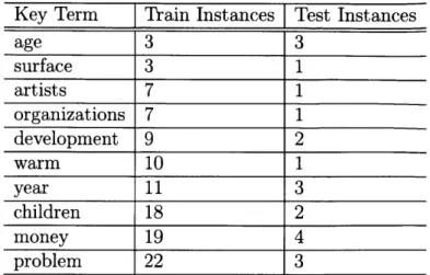
Zhang and Glass[70] developed a metric based on spoken term discovery on the TIMIT dataset, which we adopt here. For the TIMIT corpus, they decided on ten terms that

occur in both the train and test splits with varying frequency, as shown in Table 4.1.

For a given term, they use all occurences within the training split as examples, and

search for matches within the test corpus using a DTW-based system. They then

developed two metrics, inspired by information retreival evaluations, to judge the list of matches returned by the system. First is a metric called precision at N, or P N for short. This metric measures the precision of the top N matches, where N is the

Key Term Train Instances Test Instances age 3 3 surface 3 1 artists 7 1 organizations 7 1 development 9 2 warm 10 1 year 11 3 children 18 2 money 19 4 problem 22 3

Table 4.1: Key terms used for TIMIT spoken term detection evaluation. number of actual occurrences within the test corpus for the given term. The second metric is equal error rate, or EER. It measures the point at which the false positive and false negative rates are equal. In the ideal system, the top N matches are all correct; PAN is 1 and EER is 0. In the worst case scenario where we never find a match, PAN is 0 and EER is 1.

4.2

Zero Resource Speech Challenge

The study of unsupervised learning from speech has suffered from a lack of standard evaluation resources. In 2015, a group of researchers launched the Zero Resource Speech Challenge[68] to address this issue. The Challenge includes speech data in two languages (English and Xitsonga) and evaluation scripts for two different unsu-pervised learning tasks.

The Zero Resource Speech Challenge was launched as a workshop at the Inter-speech conference in September 2015. The Challenge introduced a new subword modeling task which scores frame-level representations on their phonetic content and speaker independence. This task is described in more detail in the following chapter; here, we give only a high-level overview. This task has two parts: within-speaker and across-speaker. In the within-speaker version, the goal is to find features that can distinguish two instances of the same phone from an instance of a different phone,