HAL Id: halshs-00556982
https://halshs.archives-ouvertes.fr/halshs-00556982
Preprint submitted on 18 Jan 2011
HAL is a multi-disciplinary open access archive for the deposit and dissemination of sci-entific research documents, whether they are pub-lished or not. The documents may come from teaching and research institutions in France or abroad, or from public or private research centers.
L’archive ouverte pluridisciplinaire HAL, est destinée au dépôt et à la diffusion de documents scientifiques de niveau recherche, publiés ou non, émanant des établissements d’enseignement et de recherche français ou étrangers, des laboratoires publics ou privés.
Kelly Labart
To cite this version:
Document de travail de la série
Etudes et Documents
E 2007.29
I
NTERGENERATIONAL MOBILITY INC
HINAKelly LABAR1 PhD. Student
otobre 2007 27 p
1
Corresponding author: Kelly Labar, CERDI-CNRS, Université d'Auvergne, 65 boulevard François Mitterrand, 63000 Clermont Ferrand, France; tel: +33-(0)4 73177400, fax: +33-(0)4 73177428.
Abstract:
In this paper, I study the intergenerational mobility of education and income in China. Using the CHNS database which gives information on parental educational attainment and income level, I show that there is a relatively high intergenerational mobility in China, compared to other developed and developing countries. Even if parents' social characteristics influence the child's ones, the transmission of parents' educational and income level remains low.
Nevertheless, I stress a growing impact of parents' income on the determination of children educational attainment, what can be an increasing factor of income inequality in the future. Moreover, I emphasize that parents' farming activity plays an important and significant negative role in the child's educational level.
1. Introduction
China’s economic development is regularly been understood as the reason for a raise in the country’s living standards and well-being of large parts of the population. Yet, China faces today increasing social inequalities. The income gap, but also differences in educational attainment are eye-catching. Inequalities are closely linked to the reforms the country launched by the end of the 1970’s. As a main result, they provided for a disengagement of the State from both the economic activities – the State sector plays a decreasing role in the country’s wealth production - and from the financing of certain services such as the educational system. Growing income inequalities thus derive from the enrichment of a narrow class of entrepreneurs, combined with the development of the labour market which proposes new types of employment and a new definition of wage distribution. In parallel, educational inequalities appear as the financing of schooling requires more and more the payment of the families for their children to have access to good schools and universities.
Consequently, the question resulting from this context is: Does wealth become again the major tool to provide a better environment for the children growth future? Will the richest transmit more easily their social status to the following generation or, at the contrary, will the poorest not be able to allow their children social promotion?
This paper provides for insight and a number of answers to these questions analysing intergenerational mobility in China since the movement of reforms. This topic has been studied already for previous periods of time as the political and social evolutions in this country have been particularly remarkable. This context allows a particular interesting perspective: Is China not the country, which established first the competitive examination system, with which all individuals were able, whatever their social class, to have access to the highest responsibilities, especially during the Tang and Ming hierarchical dynasties? Is it not the country which headed during the communist revolution for building an egalitarian society? To describe the background of today’s developments, the study at hand is first based on a historical perspective, which outlines the evolution of certain conflicts between the State and the families in the Chinese society. These last stress the changing role played by the family in influencing their children’s life. They also emphasise the need for State intervention in giving an equal chance to every child to have access to a social securities and benefits.
Then, the concepts of absolute and conditional mobility will be used to distinguish the fact that the child can move from one social class to another, from the fact that its parents play a role in this movement. This last impact can result, as specified in Piketty (2000), from both a higher financial investment in the child’s education by the parents, and from the social background given by the family wealth and also by its level of education.
Even if these mechanisms may not be clearly identified in this paper, first indications for the interpretation of the link between the parents and the child social status are given.
As a main tool of analyses, a longitudinal database will be used which allows to observe the evolution of intergenerational mobility focusing on the income and education dimensions for two generations.
The paper has the following structure: After the historic placement in section 1, section 2 presents the particular context of China and stresses the pertinence of studying mobility in this country today. Section 3 indicates and explains the methodology used to study this topic. Results are presented in the section 4, and section 5 concludes.
2. Intergenerational mobility: the Chinese context
China appears to be particularly interesting for the study of intergenerational mobility as a hierarchical but meritocratic historical culture underpinned the social relationship between individuals.
2.1. Before the Communist revolution
Historically, the Confucian dualistic social concept was that inequalities are inherent to any society, but these inequalities could not be based on ad-hoc hierarchy but rather on individual merit. During the Ming and Qing dynasties, upward mobility relied on the competitive examination system, which allowed individuals to have access to high level functions, whatever their parents' social status. During this period, we could also notice downward mobility due to the fact that the richest families could sometimes not assume their social responsibilities.
Ho (1959) underlines that the medieval hereditary aristocracy had been broken through the Tang dynasty (618-907 a. J.C.) during which began the competitive examination system. Social mobility started to increase from these days on to reach its maximum during the Ming dynasty (1368-1644 a. J.C.) and began thereafter to decrease. However, even if social mobility was high during these periods, it is important to stress the importance of the hierarchy in the imperial social structure, as it is one of the elements underpinning the birth of communist’s movements.
During the Republic, proclaimed in 1911 and which lasted until 1949, the country was divided between the nationalist party (Guomindang) lead by Chang Kai Chek and a communist spirit born from both the fight against the traditional Confucians hierarchy (whose symbol can be the 4th of May Movement, anti-imperialist) and the neighbour soviet 1919th revolution.
The young Republic, which decided to move towards a market economy, faced both some civil wars launched by the corrupted warlords in the north of China, and the foreign protagonists who invaded the country during this period. In parallel to the fight for national peace, a trade system was developing in China and between China and western countries, or even Japan. As consequences, a new aristocratic class, with living conditions totally opposed to the miserable countryside livelihood, emerged. Against this new unequal social system, labourers’ movements occurred in some rich towns like Shanghai. The communist party was gaining supports in the Chinese society.
During this period, it appears that social mobility was low. A corrupted and inefficient government helped the empowerment of some trading actors. The Chinese society was organized around the family. Most of the children's life events were decided by key actors of decisions in the household, who usually were the elders, or the parents. Education and marriage for example were submitted to the parental control and to their relations with other families (Engel (1984), Lindbeck (1951)). As emphasized in some modern studies on intergenerational mobility (Holmlund (2006)), assortative mating effects play an important role in diminishing mobility. The fact that the central wedding decision is in the hand of the family can reinforce the low mobility in China during the imperial and Republic periods. 2.2. Between 1949 and the end of the seventies
When the communist party and its leader Mao Tse Dong arrived at the head of the country, an important campaign against traditional hierarchy and "family individualism" (Lindbeck (1951)) aimed at reducing the historically unequal society and the family power on the child’s decisions.
Concerning the fight against inequalities, the communist period shows relative local income equalities. Nevertheless, even if within cities and villages inequalities were low, disparities between urban and rural populations or between provinces existed (Walder (1989)). However, talking about the transmission of status in terms of incomes, social mobility tended to be pretty high during the communist period. The challenge of the traditional hierarchy lead to give privileges to usually isolated social classes such as peasants what encouraged some social promotions. In parallel, Davis (1992) specifies that a particularly strong downward mobility among children of the Maoist middle class was linked to the Cultural Revolution. Walder (1989) underlines that the mobility was made thanks to drastic measures (for example, children sent to the countryside). However, another kind of social transmission was operating: the political status one, which had consequences on both social and educational status. As Walder (1989) explains, two groups were overrepresented in the best high schools: children of party officials and military officers, and children of educated middle-class background. Both of these two groups of children were in a life environment which promoted success at school. As Piketty (2000) specifies, the family background and the child cultural environment are two important determinants of intergenerational mobility. If the parents’ status influences the child's educational attainment, it also influences his income, particularly if the wages translate increasingly individual productive capacities (what will be the case in the post communist period, as we will see later).
Another goal of the Mao's system was the dissolution of families’ ties. The assimilation of the traditional family to a feudal and barbarous system justified the distance introduced between parents and their children. Many new institutions as youth league organization were created in order to make the child think by himself. Moreover, different laws allowed him to be more independent from his parents (Lindbeck (1951), Engel (1984)). In 1950, a marriage law established that "the feudal marriage system shall be abolished" (cited in Engel (1984)). Consequently, we see that the government established a system in which the child had more rights and was more independent. In the countryside, the traditional family still played a strong role in the Child's life. Different studies emphasize that these family status were not challenged as they could have undermined the support of the rural population to the party (Walder (1989)).
We see in this period (from the 1950's to the end of the 1970's), an opposition between the family and the political power. This can be a source of increasing mobility as the child is more able to prove his ability and consequently to be engaged in a better educational system. 2.3. From the reform movement to today
The reforms, launched by the end of the 1970's, have had many consequences on the social organization of the Chinese society. On the one hand, a new hierarchical structure was developing due to the marketization of the economy. On the other hand, the family began to recover a part of its place in its child's life.
Concerning the first point, with the introduction of a competitive economic system which goal was to increase efficiency, a status re-allocation occurred. As specified in Bian and al. (2005), the blue collars, seen in the Maoist period as the leading class, began to see what were the real proletarian life-conditions. They have been more and more isolated from the upper classes
constituted by managers, white collars and political elites. The party members, and particularly the State executives, have benefited from above average compensation packages and have been given privileges for social promotions and training. A kind of "embourgeoisement" appeared in this class.
The white collars, skilled individuals, and the enterprises managers have also seen their social status re-evaluated. The traditional communist spirit of equality (which implied some downward mobility for the upper-class) has consequently collapsed and some new opposition movements have been developing among the poorest populations (Bian and al. (2005)). In parallel to these structure modifications, we cannot clearly see mobility between occupations. The former drastic system of place of living registration, the Hukou, reduced the possible migrations from the countryside to the city. People could consequently not have access to the urban job market which could offer better wages and a more diversified occupational structure (Cheng and Dai (1995)). With the easing of the registration system, a higher geographical mobility can be observed and consequently, more occupational mobility can be expected with the development of the reforms.
Nevertheless, the low geographic mobility combined with a new highly hierarchical society is not prompt to help higher income mobility. The upper-class will have access to higher wages and they will consequently invest more in its children education. Moreover this fact happens in parallel to the growing place given to the family due to two major facts.
The first one is the one child policy. This policy, launched in 1979, allowing parents to have only one child, implied a new kind of intervention of the parents in their children life. As Green (1988) emphasizes, this has helped parents to become more concerned about the education of their child. The higher implication of the family in the education of its children can reduce the intergenerational mobility in China as the richest will be more able to pay for good educational services provision or help the child to be more confident in his abilities (in comparison with his peers). The direct transmission of productive ability through the child family environment is one of the determinants slowing down social mobility, as is the increase in financial investment from the parents in the child education (Piketty (2000)).
The second source of re investment of Chinese parents in the education and decisions of the child conveys exactly this last determinant.
Actually, the movement of reforms has also an impact in the educational system with the disengagement of the central government from the financing of the educational services provision (Gustafsson and Shi (2004)). Consequently, as the financing becomes more and more at the provincial levels, inequalities of education increase for two major reasons. First, a new competition between provinces in order to obtain higher budget from the central government occurred. Consequently, the provinces which have negotiated the most efficient way have been able to hire more qualified teachers and so the quality of the educational system has been different among provinces. Secondly, a system of entrance fees has been set up in order to improve the quality of the teaching and to have higher budget for other expenditures. The parents have now to invest more in the education of their child. The richest families are able to give better education both in quality and in quantity. This is nevertheless reduced by the registration system which prevents massive migrations. But the young students’ flows inside the country and between China and foreign countries tend to prove that geographical mobility is possible.
These reforms in education have had, and will have consequences on social mobility as educational attainment becomes a growing factor influencing wages because of the increasing competition between firms and the development of the private sector.
A last factor affecting the child's mobility is the legal context of the educational system. As Holmlund (2006) demonstrates, the increase of the compulsory years of schooling is a
positive factor for mobility. In China, as the political leadership has become aware of inequalities in the access to education, different measures have been taken to decrease the number of illiterates individuals and to increase the level of education of most children. One of them is the Basic Educational Law (1986) establishing nine years of compulsory school (Law (2002)).
To sum up, two major facts have to be emphasized. The first one is the role played by the political movements during the last hundred years which implied different evolution in social mobility. The second one is the relationship between the political power and the family. A strong central government can be a solution against the transmission of social status from the parents to the child. Concerning this last point, controversies emerge in the theoretical literature between the success in the increase of mobility of an authoritative political leadership observed by Boudon (1974)), and the positive impact of the democracy modelized
by Roemer (2002)2.
3. Methodology and estimation procedure
3.1 Methodology
In this paper, I am interested in two major kinds of mobility: absolute and conditional
mobility, looking at two dimensions: income and education.3
Consequently, variables of interest are the child and the parents’ educational attainment and
income. Particularly, I focus on wages both with and without bonuses.4
Absolute mobility
When I talk about social mobility, my first question is: are the children in the same social category as their parents? If the answer is no, there is, objectively, social mobility. This mobility can be the result of parents’ characteristics but also of political decisions, local policies, economic development etc. I am not looking here at the causal link between mobility and some of its determinants but at mobility between social classes, in absolute terms.
To describe the social movements between two generations of individuals, I use mobility matrices. This methodology looks at the proportion of individuals in each educational (wage) attainment category as a function of the category of educational (income) level of their parents. The hypothesis behind this tool is that no mobility is translated through high
2
Actually, Boudon (1974) argues that the only possible way to do something about persistent inequality requires a major conflict between the government and the family. At the contrary, Roemer (2002) specifies that
democracy can be a better environment than dictatorship to reduce inequalities.
3
I will also have a look at parent's occupation. Nevertheless, we will see that the variable I have access to in the database, decrease importantly the sample size. Consequently, I will not focus on the question of occupation mobility, a topic about which sociologists are more concerned.
4
I recall that the system of bonus has been implemented since the reform movement, and has as an objective to translate the productive abilities of individuals.
percentages on the matrice's diagonal. At the contrary, if higher percentages are observed above or under the diagonal, this means that children are mostly not in the same category as their parents.
Considering two dimensions of interest, that are education and income, I will have to define ordered categories as key scholar level attainment and income quartile. Moreover, it is important for the mobility matrices relative to income, to consider income conditional on the individual's (child or parents) age. This is done to take into consideration the difference of experience among parents and children which influences the level of income. This makes the
two generations' income more comparable5
.
This kind of tables is commonly used in empirical studies on intergenerational mobility both in economics and sociology (Checchi and al. (1999), Behrman and Taubman (1985), Bourguignon and al. (2001), Cheng and Dai (1995)).
Mobility matrices give a first picture of absolute mobility but it is based on arbitrary cut off between categories. Moreover, less mobility can be seen for the top and bottom categories (what is called floors and ceilings effects), due to the fact that if parents were at the top of the distribution, their child can only move downward and the contrary is true for parents coming from the bottom of the distribution (Corak and Heisz (1999)). This is why a further analysis is done.
Conditional mobility
The question here is to know if children from different social classes have the same chance to move to higher or lower category. I consequently want to know if the parents’ level of education or income is a determinant of their children social mobility considering a causality link. I have a closer look at mobility conditional on some parent's characteristics.
I am going to consider the transmission of education or wage status from parents to the child using two generations informations. Two econometric models help to study this phenomenon.
Let's consider the child's matrice of status characteristics Sc={Ec, Wc} which includes the
two vectors Ec and Wc, which represent respectively the educational level of the child and his
wage level. In a symmetric way, I define Sp={Ep, Wp} as the matrice of the two social
characteristics of the parents. 6 Consequently, the impact of the parents' status on the child's one will be studied through the relation:
Sc=f(Sp, Cc, Cp) (1)
where Cc and Cp represent control characteristics of the child and the parents.
As Sc includes two variables, I will consider two independent estimations for the child's
education and wage. Moreover, as the database I am using is from a longitudinal survey, I can use five periods of time. Consequently, the two equations which will be estimated are:
5
The estimated income will be the residuals of the following model:
yit=α+βAgeit + γ.(Ageit)²+εit
where yit is the income, and εit is the residual. 6
I could have used a dynamic model, which is equivalent to this one. But the denomination of variables using child and parent's characteristics appears clearer.
Ecit=Epit.a + ln(Wpit).b + Ccit.c + Cpit.d + vit (2)
With i reprensenting individuals and t, time periods, and where vit is the residual term.
And,
ln(Wcit)=ln(Wpit).α + Ecit.β + Ccit.γ + Cpit.δ + uit (3)
Using this model, the null hypothesis I am testing is that social transmission occurs as soon as the coefficients a and b in the equation (2) and α in the equation (3) are statistically significant. Actually, if the wage or educational level of the parents have an impact on the educational attainment or wage of the child, it is logical to consider that no conditional mobility exists. The size of the coefficient will give the magnitude of the transmission effect. I expect that, if the coefficients are significant, they will be positive. This would translate the fact that the richer or the more educated the parents are, the higher the educational level and income of the child will be.
When we look at equation (3), we see that the child educational attainment is included in the explanatory variables. This is done in order to take into account the effect of the child human capital on his wage. As the parents' level of wage influences both the child level of wage and the child level of education, the total effect of parents' wage is given by (α+b.β) as it can be seen in the following equation:
ln(Wcit)=ln(Wpit).(α+b.β) + Ccit.(γ+c.β) + Cpit.(δ+d.β) + uit (4)
It is also important to note that in the estimation of equation (3), the usual problem of the estimation of the return to education in a wage equation arises. Education is correlated with the error term generating an endogeneity bias. I will have to use instrumentation to take this problem into account. Bourguignon and al. (2001), in their study on intergenerational mobility in Brazil, use the education of the parents as the instrument, excluding it from the explanatory variables.
As I have specified above, I consider that there is no conditional mobility as soon as the coefficients on parental characteristics are significant. Nevertheless, I need to mitigate this fact considering the empirical literature on intergenerational mobility. At first, Corak and Heisz (1999) find a coefficient relative to intergenerational mobility of income in Canada of about 0.2 and significant. Nevertheless, they consider that this effect is low and that relatively good income mobility exists among the Canadian population. Holmlund (2006), for Sweden, finds a child income elasticity to parents income of about 0.16 and an increase of 0.4 years of schooling for one more parents' one. For Brazil, Lam (1999) emphasizes a 0.15 to 0.42 more years of child education for one more year of parents' education and a 0.22 one for South Africa. For the US, Behrman and Taubman (1985) find a child educational response of 0.17 to 0.20 to one more year of parents' education.
Giving the preceding results, even if we can say that as soon as parents' characteristics have an influence on the child's one, the strict conditional mobility does not exist, it is important to consider that most of the time, this situation occurs. Consequently, I will consider that a coefficient of about 0.2 of parents' income and education impact on child's ones is synonym of a relatively good level of intergenerational mobility.
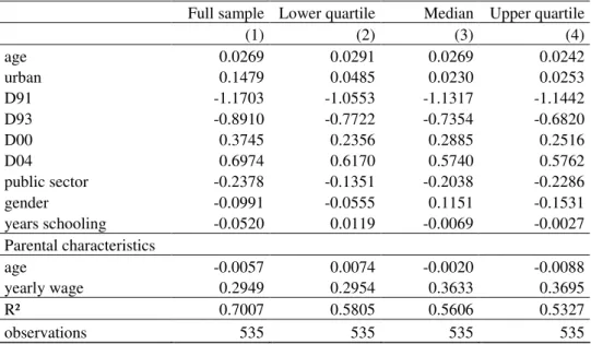
Next to this econometric model, which gives a general view of the causality between the child and the parents’ income/ education, I will check the robustness of the results looking at the impact of parents social characteristics on child's ones using quantile regressions. The usual linear regression models give an estimation of the mean conditional on the values of explanatory variables. What is interesting in quantile regression is that it allows a non
linearity between quantiles of the effect of explanatory variables on the variables of interest.7
Consequently, I will show the results relative to first 25 percent, at the median, and for the 75 quantile of educational attainment and income considering the set of right hand side variables of interest as described above.
3.2. Data and estimation problems
The data used in this paper stem from the 1991, 1993, 1997, 2000 and 2004 rounds of the China Health and Nutrition Survey (CHNS). The CHNS is an ongoing longitudinal survey that covers nine provinces (Guangxi, Guizhou, Henan, Hubei, Hunan, Jiangsu, Liaoning, Heilongjiang and Shangdong). It is organized thanks to collaboration between the Carolina Population Center, the National Institute of Nutrition Safety and the Chinese Center for Disease Control and Prevention. Although the survey is not nationally representative, these provinces were selected to provide significant variability in geography, economic development and health indicators, so that they may be considered to be generally representative of all provinces in the country.
A multistage random-cluster sampling procedure was used to draw the sample from each of the provinces. Counties in the eight provinces were stratified by income (low-, middle- and high-income tertiles) with per capita income figures from the State Statistical Office, and a weighted sampling scheme was used to randomly select four counties in each province (one low income, two middle income, and one high income). Probability-proportional-to-size sampling was used to select the sample from these units. In addition, urban areas initially not included within the county-strata were later incorporated by including the provincial capital and a low-income city from each province. Within each county, the township capital was selected and three villages were chosen randomly. Within each city, urban and sub-urban neighbourhoods were randomly selected. The same random selection procedure was used to choose the neighbourhoods for townships and villages.
The initial sample size includes 3616, 3,441, 3,875, 4,403 and 4,387 households respectively for the years 1991, 1993, 1997, 2000 and 2004. All individuals in each household were surveyed. This leads to a total sample of approximately 14,000 individuals each year. Data on occupation, income, life conditions and health have been collected. Nevertheless, some problems in the database still remain when we use it for economic topics. Some modifications are made by the survey team to improve the quality of the data for the future years.
Concerning the data relative to income, it is divided, in the survey questionnaire, between incomes issued from agriculture, business, paid activities, subventions, and remittances. I will focus my attention on incomes issued from paid activities in enterprises, firms etc. because other kinds of income, particularly agricultural incomes, are more dependent on external factors as commodity prices or weather.
7
Different methodologies have been developed since the original paper of Koenker (1978). Koenker and al. (2001) give a summary of these methods. Other useful references are Buchinsky (1994), Buchinsky (1998), Trede (1998).
Wages are measured by the monthly income. But as information on hours worked per week and weeks worked by month are available, I will be able to determine the hourly wage. Yearly bonuses, which are given an increasing weight in the determination of wages (Coady and Wang (2000)), are available for each year. Consequently, I will use the yearly wage plus bonuses as another measure of incomes.
Incomes are deflated using a provincial deflator, with distinct values for rural and urban areas.
Identification problems and estimation procedure
This survey allows us to study the intergenerational mobility under certain circumstances. I only have the parents and child educational attainment and wages in the case that the child still lives with his parents. This appears restrictive as those children can have personal characteristics influencing their level of education and wages. Particularly, I do not observe children who have moved from their town to study in other provinces or abroad. If I consider that those children are coming from the richest family, I can underestimate the amplitude of the transmission in income and education. Corak and Heisz (1999), who are using data for Canadian men, face the same issue. As they have variables which allow them to control for this selection bias, they estimate child's income elasticity to parent's income using a two stage Heckman procedure. They find no significant difference with the results which do not take
into account this problem, but the Inverse Mills Ratio is significant.8
Estimating a wage equation, I face another selection bias due to the fact that I observe the wage only for individuals who are employed. This selection is usually linked to individual characteristics which can influence the results of the wage equation. To control for this selection bias, I use the Heckman two stages procedure with a selection probit in the first stage and introduce the Inverse Mill's Ratio (IMR) in the wage equation of the second stage. Following Strauss and Thomas (1998), I use as identification variables a set of commodity prices available in the community survey from the CHNS. Given the sample size, I estimate the second stage using pooling regressions.
Another estimation problem is relative to the sex of individual. Most of the studies estimating wage equation differentiate between men and women. Nevertheless, as I lose an important number of observations considering only individuals living with their parents, I will not be able to estimate two separate education or wage equations for men and women.
Concerning the two econometric models described above, our explained variables Sc are
the child wage and educational attainment whereas our variables of interest Sp are the parents
wage and educational attainment. For these two last variables, when both the mother and the father are present in the household, I will use the average of the two levels of education and wages. When I face a mono parental household (as there are some in the data base, principally with mother only), I will take the single parent educational attainment and wage.
Actually, I consider three samples: the full sample of individuals aged by more than 16 years of age and for whom I have the level of education9; the sample of individuals who earn a wage and who are employed in an enterprise; the sample of individuals earning annual wages,
8
Giving the data, we cannot take this problem into account as we should find an identification variable which would impact the variable of the child living with his parents but would not impact the variable child's education or wage. Corak and Heisz (1999) use the Social Insurance Number assigned to individuals who filed the income tax return. We do not have this kind of random variable.
9
This sample will be the larger one as individuals who have finished their education can be unemployed, or work in household farming. Those two last categories will not be included in the two following samples.
including bonuses, and working for enterprises, or collective fishing and farming structures. For individuals working in enterprises, I have the hourly wage. This allows us to control the differences in time worked by individuals. The more general income given for enterprises and collective structures is a yearly wage. These last data will give a large picture of the income and can be particularly interesting for the impact of the parental income on the educational status of their child. The educational expenditures and investment of the parents for the education of their child are more yearly planned.
Concerning the control variables Cc, I will use the urban/rural status of the child (the
variable will take the value of 1 for urbans and 0 for rurals) as well as his living province. I do not have his province of origin and do not know precisely since when he lives in this place. This will consequently control for some province effects, as for example the educational context or policy, but not always for the environment in which the child has grown and built his personality and choices. I also introduce, in the wage equation, the child educational level as specified in equation (3). This last variable appears endogenous once I introduce it in the wage equation as some unobserved individual characteristics are in the residual and can be correlated with the educational level. This is the common bias when we estimate returns to education. As in the in the Bourguignon and al. (2001) paper, I will use the parents' education variable as an instrument for the child's education. Moreover, following Strauss and Thomas (1998), the identification variables used in the selection equation will be included in the set of instruments.
For the parents' characteristics, Cp, as Grawe (2006) underlines, it will be critical to
consider the parent's age in the equation. It is particularly important as it is possible that the parents wage is observed at an underestimated level comparing to the highest wage they will receive during their work period. The parents’ age will consequently be introduced in the circumstances variables.
Some control variables cannot be used as they would strongly and negatively affect the sample size. It is the case for the variable describing if the individual is or not a party leader, or for the individual ethnicity.
Finally, I have to precise the way I can observe the impact of the reform process on our results. Two kinds of data would allow us to take time into consideration. The first one is a huge transversal data base with information on individuals and their parents for every generation considered in the sample. I cannot consider this kind of structure here as the age range of children for whom we have parents' characteristics is too small.
The second, and the one I can use given the database, is to consider a longitudinal survey in which I have the information on the parents' education and wage for different years. As I have five observation points, I am able to look at the evolution of intergenerational mobility during the time. The figure 1 gives a picture of the date of birth and the period during which individuals were at school for every individuals considered in each survey. As we see, some of them have more or less been touched by the reform process for the education, as for the one child policy. I consider in this scheme individuals whose age is between 16 and 30 years of age as we will see in the descriptive statistics that considering only individuals who still live with their parents decrease the average age of observed individuals. I consider that the child education is beginning at five years of age.
The time evolution and the more or less high proportion of individuals considered in each survey will be the only indication which can give information on the political sources that influence intergenerational mobility. In this regard, this study gives only a first look at the evolution of intergenerational mobility in China as well as its evolution with time.
Descriptive statistics
Table 1 gives the mean and standard deviation for the principal interest variables for the three samples.
The first observation concerns the average age of the sample which is particularly young (19.6 years old). As Behrman and Taubman (1985) specified, this can have important impact on the results. The usual earning profile shows that the income tends to increase with time. A priori, the level of wage observed will be lower than the future wage the individual will earn. This is confirmed by the average wage of the parents which is, both for the hourly wage and yearly wage higher than the children one. Consequently, what I will observe will be more the impact of the parents’ characteristics on the first wage in the individual's life than on the life's average wage.
The average educational attainment of the parents is lower than the child's one. We can see that the nine years of compulsory school law seems to have a positive impact on the average evolution of the school attainment. Comparing children from the total sample with those from the sample of wage earners, we see that the last ones have a higher level of education. This is not the case for the parents. This can be the translation of a higher educational level job supply.
Concerning the children and parents levels of income, we note that the average parent's hourly and yearly wage is higher, what can be the consequence of seniority.
Considering that the parents included in the sample have worked mostly during the communist period, one can wonder how inequalities of income, in particular, could be transmitted to children, as the society was pretty egalitarian. Of course, inequalities among the same sectors of activity or the same city or even province, could be low during this period. But as written earlier, even during the Mao Tse Dong period, inequalities between urban and rural areas and between provinces existed (Walder (1989)). Consequently, two determinants can be combined to justify the existence of inequalities in my sample: the inequalities in the seniority evolution of the wage structure; a relatively unegalitarian structure when we consider a population which mixes both rural and urban individuals, or people from different provinces. To illustrate this fact, I give in the two last rows of the table 1, a measure of inequalities (the GINI coefficient10) for the sub samples of parents and children. We note a pretty high level of inequality for both of them. The GINI coefficient for parents yearly income is even higher than the one for the children one (0.4561 against 0.3917). Even if it is a simplified picture of the situation, we can see that inequalities existed, even among the workers who were employed during the communist period.
4. Intergenerational mobility
In this section, I distinguish the results relative to absolute and conditional mobility. 4.1. Absolute mobility in China
Concerning absolute mobility relative to educational attainment, we note at first, looking at the mobility matrice, given in table 2, that the diagonal does not demonstrate low mobility. At first, we see that children from parents who have only primary school (6 years of schooling) know an upward mobility to the lower middle level. We can stress to this point that this
10
The GINI coefficient gives a measure of inequalities which range is between 0 and 1, 0 standing for zero inequalities and 1 for the highest level of inequalities.
phenomenon can be particularly linked to the improvement of the educational system and to the law relative to compulsory school. This is not automatically a sign of a higher investment from the parents. This underlines the difference between what I have chosen to call "absolute" and "conditional" mobility.
When we look at other categories, we note that the diagonal figures are the highest for the parents who attained the middle school level (lower and upper) but not for the parents from the top educational level category. This can be due in part to the ceilings and floors effects stressed before.
Generally speaking, it seems that some mobility exists for education in China. Moreover, this is not only an upward mobility but also a downward mobility as we can see that for the two highest categories, a high percentage of children are in the preceding category of their parents.
Concerning the mobility matrices for incomes, given in tables 3 and 4, we note a particularly high percentage of immobility for the two extreme categories. This can be in part due to the ceiling and floor effects enounced before. But considering the whole diagonal, I emphasize a pretty high mobility as the diagonal percentages are between 23 percents and 50 percents at the maximum. Moreover, we note an upward mobility stronger than the downward one. We do not stress a huge difference between the results for the hourly and the yearly income.
These first results underline a pretty good level of absolute mobility which can be due to the higher geographical mobility allowed thanks to the hukou reforms or to the more diversified labor market which give a broader access to higher paid jobs.
4.2. Conditional mobility in China
Educational mobility
Tables 5 and 6 present the mobility in education. In both tables, the first three columns give pooling results, including the parent's education and yearly/hourly income (first column),
without parents' income (second column) and with parents farming occupation11 (third
column). As argued before, the yearly income would have more impact on the educational attainment of the child as this income source is more likely to influence education investment of the parents in the child's education than the hourly wage. However, I also give the results for the hourly wage to check for this assertion (table 6).
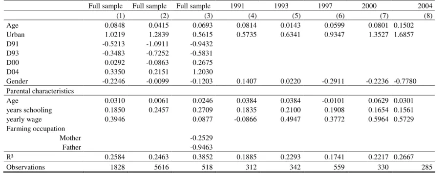
In table 5, we see that both the parents' educational attainment and income are playing a significant role in the determination of the child's level of education. As I mentioned earlier in the model, this can, at first, be considered as no conditional mobility. Nevertheless, mitigating my conclusion, I note that the impact of parents' level of education, around 0.20 more years of schooling for one more parents' years of schooling, is pretty low. Moreover, looking at the evolution with time, I underline a decreasing effect until the value of 0.1561 in 2004. The decreasing impact of parents' education on the child one is also confirmed by the results
11
In the questionnaire, the individual occupation is described thanks to an eleven choice variable. I choose to keep only the category "farming occupation" for two major reasons: first, it is an important category which can influence the child development. Living in the country side in China does not mean systematically working in a farm. Second, as many parents are participating to a farming occupation, this category allows us not to lose too many observations. Moreover, I distinguish the mother and father participation to the farming activities as giving the mean of the two would not have a clear meaning.
including parents’ hourly wage (table 6). This impact reaches its lowest value in 2004 (0.1448). These results are encouraging for the China educational system which seems to show particularly high equal opportunities for an upward mobility for the children considering their educational level.
Nevertheless, a more negative conclusion can be drawn from the income results. These last demonstrate a high impact of parents’ income on the child educational attainment. One more point of percentage of parents' income implies an increase of 0.3946 years of schooling. 12 And this alarming conclusion is more striking when we look at the time evolution which shows a growing role played by parents' income in the determination of the child level of education, reaching the highest impact of 0.5964 in 2004. This conclusion is supported by the results on hourly income. Even if, as expected, the impact of the parents' hourly wage is lower than the yearly one, the huge ascending trend is confirmed, reaching a maximum effect of 0.5013 in 2004. These results tend to support the hypothesis that the reform movement has had a negative impact on the equal access to education. As the children considered in the last periods are the one more touched by the reform process (see figure 1), the growing inequalities in the education financing are confirmed. The poorest families will not be able to provide as good and as high educational level to their children as the richest ones.
Concerning the columns including parents farming occupation, we see that both for the yearly and the hourly income specifications, the father participation to farming activities has an important and significant impact on the child educational attainment. Being a farmer implies a decrease of 0.9463 years of schooling when I include the parents' yearly income (which is no more significant), and a decrease of 1.2383 years of schooling when we consider the parents' hourly wage. These impacts are correlated with the urban impact as we note a decreasing coefficient on the urban variable once the father's farming occupation is introduced. This appears logical as most of the farming occupations are done in the countryside. But this is important and interesting to note when we consider the time trend of the impact of being an urban resident. I cannot include the parents' occupation impact during time as I would lose too many observations. But when we look at the impact of the urban variable, we note a increasing, significant and important effect of it. The impact goes from 0.5735 in 1991 to 1.6857 in 2004. This effect can include two major facts: living in the urban area allows children to have access to higher education; parents' occupations in cities are less farming ones what tend to favour children.
Finally, it is important to stress that the effect of farming occupation is higher than the income effect. These first conclusions relative to parents' occupation would be a topic to
investigate in the future, using more accurate and available data.13
The results of quantile regressions are presented in tables 7 and 8. An interesting phenomenon is to be noted both when we consider yearly and hourly wage. The impact of parents' characteristics is more and more important with the increase in the child school attainment. This means that the parents' social status in terms of education and income is more transmitted for the top social classes. This appears logical as the Chinese educational system becomes more and more elitist with the educational level children want to reach. Parents must invest a higher share of their budget and that is also why the pressure on the young students is so high.
Looking at the urban variable, we note an increase of its impact with the increase in educational quartile. This confirms the fact that living in cities gives better opportunities to have access to higher educational degrees.
12
The wage variables are always considered in logarithm.
13
To my knowledge, no such data are available yet. Some database give information on occupations, others allow the intergenerational mobility studies.
Concerning the particularity of quantile regression which allows seeing the non linearity of impacts of our variable of interest, we see an important cut off of the parents’ educational attainment impact between the median group and the 75 quantile and a cut off of the parents' income impact between the first quartile and the median group. Consequently, better educated parents play a role mostly during the last years of child's schooling but a lower budget constraint seems to decrease schooling opportunities early in the school system.
Income mobility
Concerning income mobility, the first stage Heckman procedure probit results show that our identification variables are jointly significant.
To estimate the wage equation, I am using pooling regressions as using a fixed effects model would imply a loss of observations. The sample is already not large and consequently, I also will not be able to do estimations by period.14 Results are presented in the tables 9 and 10. We remember that we have two effects of the impact of the parents' income on the child's one. The direct one (α in equation (2)), is given directly by the coefficients on the various parents' wage included in the table; and the indirect effect, which is the coefficient on the yearly/hourly income of the parents on child's educational attainment, multiplied by the coefficient on the yearly/hourly income of the parents on the child's one (β.b in equation 3)). I add those coefficients in the table, noted yearly/ hourly wage indirect effect.
For the hourly wage, the OLS results show a positive and significant impact of the parents' hourly wage on the child hourly wage. One percent more in the parents' income implies a direct effect of 0.2306 percent more in the child income (table 9). We see that the indirect
effect is positive and small. These first estimation results are confirmed by the 2SLS results15
which give an impact of 0.2589. A relatively higher impact is found for the yearly income which reaches an effect of 0.2949 in the 2SLS estimations. Considering the literature on intergenerational mobility, these impacts seem pretty low, showing a correct level of income mobility in China. This tends to support the hypothesis saying that the communist environment favours a society in which inequalities remain low and social status transmission
in terms of income, is not too much important.16
In columns 4 and 8, the mother's and father's farming occupation are included. We note an important decrease in the number of observations which mitigate the significance of our results. Nevertheless, the impacts of parents' incomes are decreasing both for the yearly and the hourly ones even if the coefficients on farming occupations are not significant. This proves again the role played by parents work activity in the intergenerational mobility in China.
Concerning the econometric methodology used here, we can see that our instruments are not rejected by the Hansen test for the specification including hourly income, and without
14
To take time into account for the income mobility, I introduced the parents' income variables multiplied by the time dummies. This did not give significant results. That is why I haven't introduced them it in the table.
15
The results of the 2SLS estimations of the tables 9 and 10 are given using the parents' educational level as instrument for the child’s one. Following Strauss and Thomas (1998), I also introduce the identification variables of the selection probit (commodity prices) as instrumental variables. I checked for the smoking habit variable but this implies a strong decrease of the number of observations and moreover this variable did not appear to affect significantly the child educational attainment.
16
As I am not able to identify the effect of reforms for the income mobility, we cannot know if they have had a negative impact on mobility during time.
parents farming occupations. But they appear fragile for the specifications including the yearly income.17
The inverse Mills ratio included to control for the selection appears non significant for all the specifications chosen.
Considering the quantile regression results, which can be found in tables 11 and 12, a much lower mobility is observed for the yearly income for the median and 75 quartile groups. One percent more in parents' yearly income implies an increase of 0.36 percent in child yearly income. This is interesting as the yearly income includes bonuses. Does that mean that bonuses are not distributed according to the employees' abilities? No clear element allows us to conclude this way.
5. Conclusion
Using a longitudinal survey realized in nine Chinese provinces, I have studied the intergenerational educational and income mobility in China. The specificity of the political as well as the economic context of this country shows the necessity of studying the mobility in the Chinese society.
Given that I have information on educational attainment and income for both parents and child only for individuals who live with their parents, the results of this study are a first step to the quantification of the mobility in China.
I have emphasized the existence of absolute mobility in education thanks to the use of mobility matrices. This absolute mobility is completed by a relatively high conditional mobility in education considering the impact of parents' education (one more year of parents education leads to approximately 0.2 more year of child education). Nevertheless, worrying conclusion have been drawn from the role played by parents' income on the child educational attainment with a highest impact of 0.5964 more year of child education for an increase of 1 percent in the parents' yearly income. This observation tends to support the recent literature developed around the increase in education inequalities due among other to the increase in entrance fee for colleges and universities (Gustafsson and Shi (2004), Wan and Zhang (2006), Zhang and Kanbur (2005)). I have also underlined the role played by parents' occupations and particularly the negative impact of the parents’ participation to farming activity. Moreover, this effect appears more important than the one linked to the parents' income. Inequalities of access to education in rural areas seem central for the child educational attainment.
Concerning income mobility, one percent increase of parents' incomes implies a 0.25 to 0.29 percent increase in child's income. These figures are not very high once we consider the literature on income mobility in developed or developing countries. Nevertheless, I have pointed out the more important impact of parents' yearly income for the median and 75 quartile groups. Given that yearly incomes include bonuses, it would be interesting to have more details on the way they are distributed.
Even if my results are submitted to the data structure, I can conclude that the egalitarian political regime has pretty well succeeded in re-setting the hierarchical and traditional system which consisted in a small intergenerational mobility in the social status of individuals.
17
To our knowledge, and given the database, no significantly good instruments have been used until now. The one I am using here are supported by other studies but these ones concern other countries Bourguignon and al. (2001), Strauss and Thomas (1998))
Nevertheless, the increasing inequalities in income and in education financing tend to mitigate this encouraging conclusion. Consequently, political concerns should focus more on the reduction of inequalities to create an "equal playing field".
A larger survey with more detailed and larger sample on the different generations’ income and educational attainment would be highly useful to confirm these results.
Bibliography
Behrman, J. and Taubman, P. (1985), 'Intergenerational Earnings Mobility in the United States: Some Estimates and a Test of Becker's Intergenerational Endowments Model', The
Review of Economics and Statistics 67(1), 144-151.
Bian, Y., Breiger, R. Davis, D. and J. Galaskiewicz (2005), 'Occupations, Class, and Social Networks in Urban China', Social Forces 83(4), 1443-1468.
Boudon, R. (1974), Education, Opportunity and Social Inequality, New york: Wiley.
Bourguignon F., Ferreira F. and Menendez, M. (2001), 'Inequality of Outcomes, Inequality of Opportunities and Intergenerational Education', .
Buchinsky, M. (1998), 'Recent Advances in Quantile Regression Models: A Practical Guideline for Empirical Research.', The Journal of Human Resources 33(1), 88-126.
Buchinsky, M. (1994), 'Changes in the U.S. Wage Structure 1963-1987: Application of Quantile Regression', Econometrica 62(2), 405-458.
Checchi D., Ichino A. and Rustichini, A. (1999), 'More Equal But Less Mobile? Education Financing and Intergenerational Mobility in Italy and in the US', Journal of Public Economics
74, 351-393.
Cheng, Y. and Dai, J. (1995), 'Intergenerational Mobility in Modern China', European
Sociological Review 11(1), 17-35.
Coady, D. and Wang, L. (2000), 'Equity, Efficiency, and Labor-Market Reforms in Urban China : The Impact of Bonus Wages on the Distribution of Earnings', China Economic
Review 11(3), 213-231.
Corak, M. and Heisz, A. (1999), 'The Intergenerational Earnings and Income Mobility of the Canadian Men: Evidence from Longitudinal Income Tax Data', The Journal of Human
Resources 34(3), 504-533.
Davis, D. (1992), '"Skidding": Downward Mobility Among Children of the Maoist Middle Class', Modern China 18(4), 410-437.
Engel, J. W. (1984), 'Marriage in the People's Republic of China: Analysis of a New Law',
Journal of the Marriage and the Family 46(4), 955-961.
Grawe, N. D. (2006), 'Lifecycle Bias in Estimates of Intergenerational Earnings Persistence',
Green, L. W. (1988), 'Promoting the One-Child Policy in China', Journal of Public Health
Policy 9(2), 273-283.
Gustafsson, B. and Shi, L. (2004), 'Expenditures on Education and Health Care and Poverty in Rural China', China Economic Review 15(3), 292-301.
Ho, P. (1959), 'Aspects of Social Mobility in China, 1368-1911', Comparative Studies in
Society and History 1(4), 330-359.
Holmlund, H. (2006), 'Intergenerational Mobility and Assortative Mating Effects of an Educational Reform', .
Koenker, B. and G., Basset (1978), 'Regression Quantiles', Econometrica 46(1), 33-50.
Koenker, R. and Hallock, K. (2001), 'Quantile Regression', Journal of Economic Perspectives
15(4), 143-156.
Lam, D. (1999), 'Generating Extreme Inequality: Schooling, Earnings, and Intergenerational Transmission of Human Capital in South Africa and Brazil', .
Law, W. (2002), 'Legislation, Education Reforms and Social Transformation: The People's Republic of China's Experience', International Journal of Educational Development 22, 579-602.
Lindbeck, J. M. H. (1951), 'Communist Policy and the Chinese Family', Far Eastern Survey
20(14), 137-141.
Piketty, T. (2000), Theories of Persistent Inequality and Intergenerational Mobility. Roemer, J. E. (2002), 'Does Democracy Engender Inequality?', .
Strauss, J. and Thomas, D. (1998), 'Health, Nutrition and Economic Development', Journal of
Economic Literature 36(2), 766-817.
Walder, A. G. (1989), 'Social Change in Post-Revolution China', Annual Review of Sociology
15, 405-424.
Wan, G. and Zhang, X. (2006), 'Rising Inequality in China', Journal of Comparative
Economics 34, 651-653.
Zhang, X. and Kanbur, R. (2005), 'Spatial Inequality in Education and Health Care in China',
Figure 1:Chronology of the most important reforms that have an impact on educational level and incomes.
1961 196 3 196 7 1970 1974
1966 1968 1972 1975 1979 1979: Economic reforms and The One
Child Policy are lauchned 1981: Begin of the educational reforms 1986: Law on cumpolsory school 1991 199 3 199 7 2000 2004
Birth period giving the year of survey
Education period giving the year of survey and considering education begin at five years old.
Table 1: Summary statistics
Total Yearly Wage earners Hourly Wage earners
Observations 1828 535 347
mean standard mean standard mean standard
deviation deviation deviation
Children characteristics hourly wage 2.4943 3.3045 yearly wage 3299.538 4722.908 Age 19.6682 2.9796 21.5850 2.8782 21.7328 2.8836 Gender 0.5322 0.4991 0.5084 0.5004 0.4928 0.5007 public sector 0.6822 0.4660 0.6571 0.4754 urban sector 0.4075 0.4915 0.4056 0.4915 0.4207 0.4944 years schooling 9.9404 2.4044 10.2131 2.6079 10.3746 2.7388 Parent's characteristics hourly wage 3.1290 4.7596 yearly wage 3733.575 4310.799 Age 46.9633 5.1072 48.7102 5.5315 48.6125 5.2172 years schooling 7.3936 3.4836 7.0701 3.5701 7.2579 3.7847 GINI coefficient Child income 0.3917 0.4567 Parents' income 0.4561 0.4337
Table 2: Educational mobility matrice
Child's educational status
Parental education primary lower upper college Observations status (% total observations) school middle middle
primary school 10.06 60.95 25.15 3.85 676
lower middle 4.51 47.09 40.55 7.85 688
upper middle 2.74 26.22 56.10 14.94 328
college 0.00 7.35 59.56 33.09 136
Table 3: Hourly wage mobility matrice
Child hourly earnings quartile
Parent's hourly earnings Bottom 2nd 3rd top Observations quartile (% total observations)
bottom 49.35 37.66 11.69 1.30 77
2nd 23.81 23.81 34.52 17.86 84
3rd 17.11 17.11 34.21 31.58 76
top 15.29 18.82 15.29 50.59 85
Table 4: Yearly income mobility matrice
Child yearly earnings quartile
Parents's yearly earnings bottom 2nd 3rd top Observations quartile (% total observations)
bottom 52.76 31.50 8.66 7.09 127
2nd 25.20 22.83 35.43 16.54 127
3rd 15.08 16.67 31.75 36.51 126
Table 5: Intergenerational mobility in education. Parents' income measured by the yearly income.
Full sample Full sample Full sample 1991 1993 1997 2000 2004
(1) (2) (3) (4) (5) (6) (7) (8) Age 0.0848 0.0415 0.0693 0.0814 0.0143 0.0599 0.0801 0.1502 Urban 1.0219 1.2839 0.5615 0.5735 0.6341 0.9347 1.3527 1.6857 D91 -0.5213 -1.0911 -0.9432 D93 -0.3483 -0.7252 -0.5831 D00 0.0292 -0.0863 0.2675 D04 0.3350 0.2151 1.2030 Gender -0.2246 -0.0099 -0.1203 0.1407 0.0220 -0.2911 -0.2236 -0.7780 Parental characteristics Age 0.0310 0.0061 0.0246 0.0384 0.0384 -0.0101 0.0629 0.0301 years schooling 0.1850 0.2457 0.2709 0.1835 0.2100 0.1908 0.1654 0.1561 yearly wage 0.3946 0.0877 -0.0866 0.4947 0.3772 0.5964 0.5729 Farming occupation Mother -0.2529 Father -0.9463 R² 0.2584 0.2463 0.3852 0.1885 0.2293 0.1741 0.2217 0.2667 Observations 1828 5616 518 312 342 559 330 285
OLS estimator (Huber-White standard errors in parentheses).
D91, D93, D00 and D04 are dummy variables which take the value of 1 respectively for the years 1991, 1993, 2000 and 2004, and 0 elsewhere. 1997 is taken as the year of reference. All incomes are expressed in natural logarithme.
Table 6: Intergenerational mobility in education. Parents' income measured by the hourly income.
Full sample Full sample Full sample 1991 1993 1997 2000 2004
(1) (2) (3) (4) (5) (6) (7) (8) age 0.0898 0.0415 0.0676 0.0836 0.0113 0.0468 0.0949 0.1594 urban 1.0312 1.2839 0.4697 0.5245 0.7321 0.9153 1.4057 1.6636 D91 -0.4428 -1.0911 -0.4004 D93 -0.2239 -0.7252 -0.1668 D00 0.0247 -0.0863 0.2502 D04 0.4550 0.2151 1.2439 gender 0.1890 0.0099 0.0210 -0.1542 -0.0987 0.2656 0.2442 0.6821 Parental characteristics age 0.0286 0.0061 0.0240 0.0338 0.0477 -0.0061 0.0579 0.0260 years schooling 0.1896 0.2457 0.2831 0.1776 0.2396 0.1881 0.1719 0.1448 hourly wage 0.2637 0.4521 -0.1503 0.1617 0.3130 0.4004 0.5013 Farming occupation Mother -0.2276 Father -1.2383 R² 0.2505 0.2463 0.4028 0.1796 0.2338 0.1692 0.1987 0.2484 observations 1739 5616 479 300 318 538 318 265
OLS estimator (Huber-White standard errors in parentheses).
D91, D93, D00 and D04 are dummy variables which take the value of 1 respectively for the years 1991, 1993, 2000 and 2004, and 0 elsewhere. 1997 is taken as the year of reference. All incomes are expressed in natural logarithme.
Table 7: Intergenerational mobility in education: quantile regressions. Parents' income measured by the yearly income.
Full sample
Lower
quartile Median Upper quartile
(1) (2) (3) (4) age 0.0252 0.1078 0.0378 0.1568 urban 1.0704 0.6159 0.9051 1.0419 D91 -1.1534 -0.2647 -0.1699 -0.7580 D93 -0.7541 -0.1510 -0.1118 -0.6771 D00 0.2151 -0.0157 0.1042 -0.3306 D04 0.5393 0.0829 0.1988 0.1775 gender -0.5389 0.1673 0.2082 0.2493 Parental characteristics age 0.0167 0.0152 0.0292 0.0469 years schooling 0.2654 0.1078 0.1189 0.1590 yearly wage 0.3269 0.2407 0.3198 0.3398 R² 0.2584 0.0376 0.1440 0.1662 observations 1828 1828 1828 1828
Table 8: Intergenerational mobility in education: quantile regressions. Parents' income measured by the hourly income.
Full sample
Lower
quartile Median Upper quartile
(1) (2) (3) (4) age 0.0252 -0.0024 0.0418 0.1799 urban 1.0704 0.5872 0.9611 1.1186 D91 -1.1534 -0.2708 -0.0902 -0.5760 D93 -0.7541 -0.1422 0.0289 -0.4650 D00 0.2151 -0.0553 0.0554 -0.3087 D04 0.5393 0.1262 0.2605 0.4584 gender -0.5389 0.1555 0.1595 0.1750 Parental characteristics age 0.0167 0.0127 0.0283 0.0438 years schooling 0.2654 0.1032 0.1160 0.1555 hourly wage 0.3269 0.1263 0.2358 0.2456 R² 0.2505 0.0306 0.1428 0.1598 observations 1739 1739 1739 1739
Table 9: Intergenerational income mobility. Parents' income measured by the hourly income. probit OLS 2SLS 2SLS (1) (2) (3) (4) age 0.1246 0.0417 0.0474 0.0225 urban 0.3858 0.0636 0.1050 0.0415 D91 0.1770 -1.1747 -1.1662 -1.1050 D93 -0.6585 -0.8362 -0.8565 -0.7108 D00 -0.3044 0.2171 0.2363 0.2448 D04 1.1441 0.5779 0.6767 0.4401 public sector 1.7010 -0.1911 -0.0751 -0.4450 gender 0.1289 -0.0987 -0.0837 -0.0795 years schooling -0.0541 0.0007 -0.0309 0.0404 Parental characteristics age -0.0085 -0.0008 -0.0006 0.0037 years schooling -0.0007 yearly wage hourly wage 0.2206 0.2306 0.2589 0.1798 Farming occupation Mother 0.1550 Father 0.0859
yearly wage indirect effect
hourly wage indirect effect 0.0002 -0.0140 0.0183
Identification variables
Commodity prices
F-test of joint significance (p-value) χ²=12.50
Inverse Mills ratio:
λit 0.0476 0.1430 -0.1290
R² 0.3595 0.7581 0.7539 0.7573
Hansen test of the overidentifying χ²=7.65 χ²=13.577
restrictions (p-value) 0.2650 0.0347
observations 531 347 347 177
Selection probit, OLS and 2SLS results estimator (Huber-White standard errors in parentheses). For the probit estimations, figures in brakets are the marginal effects. All incomes are expressed in natural logarithme.