Neurite Tracing With Object Process

HAL Id: hal-01366490

https://hal.sorbonne-universite.fr/hal-01366490

Submitted on 14 Sep 2016

HAL is a multi-disciplinary open access

archive for the deposit and dissemination of

sci-entific research documents, whether they are

pub-lished or not. The documents may come from

teaching and research institutions in France or

abroad, or from public or private research centers.

L’archive ouverte pluridisciplinaire HAL, est

destinée au dépôt et à la diffusion de documents

scientifiques de niveau recherche, publiés ou non,

émanant des établissements d’enseignement et de

recherche français ou étrangers, des laboratoires

publics ou privés.

Sreetama Basu, Wei Tsang Ooi, Daniel Racoceanu

To cite this version:

Sreetama Basu, Wei Tsang Ooi, Daniel Racoceanu. Neurite Tracing With Object Process. IEEE

Transactions on Medical Imaging, Institute of Electrical and Electronics Engineers, 2016, 35 (6), pp.

1443-1451. �10.1109/TMI.2016.2515068�. �hal-01366490�

Neurite tracing with object process

Sreetama Basu, Institute of Biology, ´

Ecole Normale Sup´erieure. Paris 75005, France.

Wei Tsang Ooi, School of Computing, National University of Singapore. Singapore 117417, Singapore.

Daniel Racoceanu, Sorbonne Universit´es, UPMC Univ Paris 06, CNRS, INSERM, Laboratoire d’Imagerie

Biomedicale, Paris 75013, France.

Abstract—In this paper we present a pipeline for automatic analysis of neuronal morphology: from detection, modeling to digital reconstruction. First, we present an automatic, unsu-pervised object detection framework using stochastic marked point process. It extracts connected neuronal networks by fitting special configuration of marked objects to the centreline of the neurite branches in the image volume giving us position, local width and orientation information. Semantic modeling of neuronal morphology in terms of critical nodes like bifurcations and terminals, generates various geometric and morphology descriptors such as branching index, branching angles, total neurite length, internodal lengths for statistical inference on characteristic neuronal features. From the detected branches we reconstruct neuronal tree morphology using robust and efficient numerical fast marching methods. We capture a mathematical model abstracting out the relevant position, shape and connec-tivity information about neuronal branches from the microscopy data into connected minimum spanning trees. Such digital reconstruction is represented in standard SWC format, prevalent for archiving, sharing, and further analysis in the neuroimaging community. Our proposed pipeline outperforms state of the art methods in tracing accuracy and minimizes the subjective variability in reconstruction, inherent to semi-automatic methods. Index Terms—Neuron morphology analysis; Marked point processes; Fast marching; Neurite tracing; Digital reconstruction.

I. OVERVIEW

A. Introduction

Comprehending the complex structure and connections of neurons is key to the study of brain development and function-ing. Advances in microscopy imaging technology has enabled us to capture neuronal morphology in unprecedented high res-olutions. But, the huge volume of rich and heterogeneous data generated, makes expert manual analysis tedious, subjective and prohibitively time consuming.

Till date, the only organism to have a fully described connec-tome is the roundworm (C. Elegans) [38]. It is a nominally evolved organism with a primitive neuronal network presenting only a small subset of the morphological variations and com-plexity exhibited in higher organism. Recently, many efforts are underway to generate detailed neuronal atlases of common lab animals such as rats, mice and fruit-flies to facilitate in silico experimentation. At the core of such efforts lies the challenging task of detection and reconstruction of neuronal branches from large 3D microscopy data stacks acquired by various imaging modalities.

Neurons exhibit a tree-like pattern of tubular branches at light microscopy resolutions. To extract the positional, shape and connectivity information of the neuronal branches is a difficult task. Firstly, the branches present a wide variation of scale and shape from thin, wispy filaments to thick primary

branches. Secondly, the branches take on a beaded appearance with inhomogeneous intensity, gaps and discontinuities due to imperfect staining and exhibit poor contrast with fuzzy, undefined boundaries distorted by microscopy PSF. Imaging artefacts, such as structured noise, gradation caused by uneven illumination, background clutter due to other labelled organelle — impose further challenges for automatic analysis. Often limiting resolution in Z axis (perpendicular to imaging plane), induces a 2D projection effect obscuring branch connectivity and misappropriating branch length. It is known to have caused expert manual reconstructions to contain loops in the neuronal arborization. These are treated as Gold Standards (GS) to evaluate performance of automatic algorithms. It is a particularly significant problem as automatic reconstructions are then penalized for performing better than the tracing methods producing incorrect loopy reconstructions.

B. Related Works

Tubular structures such as neurites, vasculature networks, bronchial airways are abundantly encountered in biomedical imaging. The connected centerlines of these tubules provide an accurate representation of the topologies. Existing neurite tracing methods mostly fall into 2 broad categories — global segmentation and local exploratory methods.

The global methods are mainly skeletonisation or medial axis representations of a segmented neurite image [3], [27], [41], [39], [29]. These methods are extremely sensitive to the segmentation results. A good segmentation of the neurite is difficult to achieve due to imaging artifacts, noise and non-uniform staining of neuronal fibres. Subsequent pruning of the skeletal tree is necessary to remove loops and spurs adding false length to the neurites. Traditional segmentation techniques fail to generate a connected 1 pixel-wide centreline representation of the neurite topology. Often, heuristic post processing or even manual intervention, is required to merge disconnected components into graph-theoretic representation of nodes as bifurcations, terminals and intermediate paths. Moreover, the memory requirements of global methods are, generally, exceptionally high making them unattractive choices for large data sets (and limiting them to 2D data only [3]). The complexity and variability of neurons make it painstaking to extract morphological and geometrical parameters (e.g., total neurite length, the number of branches, branch angle) to describe the neurons.

In contrast to global methods, explorative neurite tracing con-nects paths of maximum neuriteness voxels locally between sets of seed points incrementally to extract the global neurite

structure [35], [8], [37], [30]. A common drawback of these algorithms is their dependence on availability and quality of seed points. Often, interactive tracing is required to select the optimal seed points [21]. Traditionally, multi-scale Eigen analysis [12], in combination with gradient information [17] or intensity ridge traversal [1] are used to detect seed voxels on tubule centerlines. These multiscale filters find voxels maximizing a vesselness measure by collecting responses over a range of filter scales. However, Hessian-based filters, eg. Frangi vesselness filters, fail at critical junctions and bifur-cations where the neuronal morphology deviates significantly from expected tubular cross-sections. They are also sensitive to presence of adjacent structures. Hence, a scale-orientation space non-maxima suppression of the filter response fails to generate seeds on the topological centreline of the neurite branches for subsequent connectivity inference.

Recently, various supervised machine learning techniques modeling the centreline detection problem as a classification task have been proposed in the literature [32], [34]. These methods use a cascade of weak binary classifiers for extracting centreline voxels. However, they are not strongly discrimi-native between pixels on and close to centerlines. This is because the complex geometric and radiometric variability, both natural and induced by imaging and staining artefacts, present in neurites are difficult to enumerate and learn. Parametric deformable Active Contour are frequently used for tracing neuronal branches between pairs of seed points [8], [37]. The intrinsic shortcoming of snake based methods is their sensitivity to initialization and background noise, in addition to its inability to deal with topological adaptation such as splitting or merging of branch parts. Active contours require very precise initialization to avoid being trapped by local energy minima. Extensive preprocessing is required for selection of candidate voxels for initialization of snakes and dynamic re-parameterization is necessary to accurately recover the object centreline. Hence, recently level sets and the numerically efficient fast marching methods, that can avoid the mentioned drawbacks, have gained popularity for neurite tracing [26], [28], [13]. A second class of local explorative methods — the Iterative Model Fitting— fits a cylindrical neurite-like kernel, between sets of detected seed points [42]. These methods are computationally efficient since it performs a localized search by matching templates at different orientations at the end of already detected segments. But the high cross-sectional morphology variability does not allow such shape averaging. The neuronal fibres are approximate tubules often of irregular cross-section depending on “XY” and “Z” data acquisition resolution. Moreover, such cylinder or tubule like templates perform poorly at junctions or bifurcations.

Existing methods are mostly semi-automatic, requiring user interaction for resolving ambiguities and merging fragmented traces. The growing literature and many recent survey papers on the topic [25], [11], [33] is evidence that automated neu-ronal reconstruction is still an open and challenging problem.

C. Contribution

In this work, we propose a fully automatic pipeline for analysis of neuronal tree morphology: from detection,

seman-tic modeling to digital reconstruction. Components of this pipeline has been previously published [4], [5], [6]. Starting with an unsupervised object detection methodology to extract neuronal fibres from 3D image stacks, we integrate detection, modeling and connectivity inference into an automated neurite tracing pipeline. We employ stochastic marked point process and energy function suitably adapted to detection of tubular structures. We incorporate high level semantics of branching arbor patterns as priors in our model to generate a meaningful and precise description of the neuronal tree morphology. This enables generation of characteristic geometric and topological features, such as branching index, branching angles, total neu-rite length, internodal lengths, branch curvature, tapering rate etc., for statistical inference on neuronal parameters. Special priors enable to interpolate the continuity of disjoint, weakly labeled sections of neuronal branches. The parameter-free fast marching method verifies the connected minimal paths using image potential. We order the geodesic curves representing the branch topologies into a directed minimum spanning tree (MST) hierarchy. The underlying numerical principles make it fast, memory efficient and robust. Thus, our method captures the inherent graphical structure of neuronal arborization. We compare the performance of our proposed pipeline against the state of the art on data sets featured in the DIADEM challenge using multiple standard metrics. Overall, our method improves accuracy of automated reconstruction and further minimizes the subjective variability of existing interactive and semi automatic reconstruction tools. This digitized represen-tation of both morphology and connectivity information of neuronal trees from the noisy unstructured microscopy data can facilitate further analysis and archiving.

The rest of the article is organized as follows: In section II we present a brief overview of our reconstruction pipeline. Section III introduces the marked point process methodology and explains our object detection model. In section IV, we present our reconstruction method. Section V contains the experimental results and finally we conclude in section VI.

II. PROPOSEDMETHOD

Our aim is to capture the positional and connectivity in-formation of neuronal morphology into an analytic model. We solve this problem by formulating neuronal branches as a special configuration of an object process. It offers the advantage of imposing geometric shape and point interaction constraints on the set of points describing the spatial distribu-tion of data. The neuronal structure is described by an optimal configuration of the marked point process objects fitted to the tubular branches. The centreline co-ordinates and corre-sponding scale and orientation information is obtained in an automatic, unsupervised manner requiring no user interaction. Finally, a tree traversal of the detected points on the neuron generates a minimum spanning tree representation.

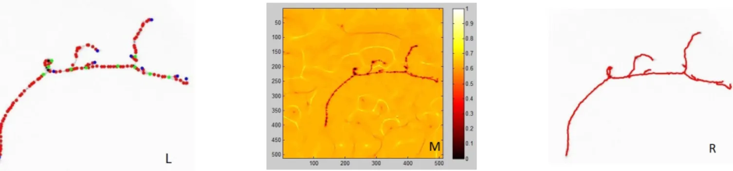
Refer Fig. 1 for an overview of the reconstruction pipeline. We detect seed points spaced uniformly on the neurite branches by a Marked Point Process model (Fig. 1(a)). The automatically generated seeds, with bifurcation nodes in green, terminals in blue, and anchor nodes along branches in red, are used to fre-quently re-initialize the marching front on the speed map. The

Fig. 1: Reconstruction pipeline. L: The final MPP configuration - bifurcation nodes (green), terminal nodes (blue) and anchor nodes (red) on branches. M. The speed image for front propagation. R. Reconstructed neuron with branch segments approximated by minimal paths. Gradient Vector Field (GVF) based speed image (Fig. 1(b))

guides the front propagation to have maximum speed on the branch centrelines. The resulting minimum spanning tree is shown in (Fig. 1(c)). The neuron tree reconstruction by fast marching models the branches by the geodesic curves representing the medial axes of their topologies. Our algorithm goes through the following steps:

1. First we detect the neuronal branches by fitting the optimal MPP object configuration to the neurite centrelines.

2. Now we define an adjacency matrix with all MPP objects as nodes and edges defined by euclidean distances between nodes within attractive distances of each other according to the MPP final configurations. We perform a topological sort of the automatically generated nodes into a tree-like hierarchy using Kruskal’s algorithm [18]. Now we use fast marching to verify the edges of the tree by extracting them as geodesic minimal paths.

3. We compute a Gradient Vector Field (GVF) based speed map of the data volume to guide Front Propagation (FP). 4. From a start node, the front propagates on the speed image until it reaches the end node. A gradient descent on the arrival time map of the front connecting the start and end nodes extracts the geodesic path between them in the form of the medial axis of the branch topology. For the erroneous edges in our tree, the minimal geodesic path fails to connect the 2 nodes due to the image potential based speed map. We remove the corresponding end nodes of the detected false edges. 5. We re-initialize our front and repeat Step 4 until all nodes are exhausted. Thus, our reduced node list gives a minimum spanning tree (MST)description of the neuronal data by modeling the neurite branches by minimal geodesic paths. In the following sections, we explain in further detail the individual steps involved.

III. DETECTION

In this section, we describe the stochastic framework that enables a flexible object process to sample special configura-tions of objects fitted to the voxels of maximum medialness measure on the image volume. In [2], the Point Process models were introduced to exploit random fields whose real-izations are configurations of random points describing spatial repartition of data. It is particularly useful for addressing spatial relation and configuration modeling problems for high dimensional, high resolution data.

A. 3D Marked point process: notations, definitions

Marked point process (MPP) is an augmented point process, where each point xi existing in a bounded, connected subset

K= [0, Xmax] × [0,Ymax] × [0, Zmax] of V3, the image domain,

is associated with additional parameters (marks) M = [mi] to

define an object ωi= (xi, mi). Here, xi∈ K and mi∈ M and the

marked point process Y is defined on K × M. A countable, unordered set of points in Y is called a configuration. The configuration spaceof the objects is given by:

Ω = ∪∞_n=0Ωn, (1)

where Ω0 is the empty set, each Ωn, n ∈ N is a configuration

containing n objects and γn∈ Ωn, γn= {ω1, . . . , ωn}. Note, that

n can be arbitrary, and in the following sections of the paper the elements of configuration γ ∈ Ω (with an arbitrary number of elements) will be denoted as {ωi}, where i = 1 . . . n.

The Marked Point Processes are defined by their probability density w.r.t. the reference Poisson process. Given a real, bounded function U (γ) in Ω, the Gibbs distribution µβ(γ) in

terms of the probability density p(γ) =dµβ

dλ (γ) w.r.t.

Lebesgue-Poisson measure λ on Ω is defined as: p(γ) =z

|γ|

Zβ

exp[−βU (γ)]. (2) Here, γ represents the configuration of objects, z, β > 0 and Z_β is a normalizing factor:

Z_β=

Z

γ ∈Ω

z|γ|exp [−βU (γ)]dλ (γ). (3) Eq. 3 shows how these models are defined on huge configura-tion spaces over unknown number of objects. The principle for estimating such very high-dimensional integrals is to define a Markov Chain Monte Carlo (MCMC) simulation converging to a target distribution. By including a simulated annealing scheme, the chain converges to the Maximum A Posteriori (MAP) estimate, which is the configuration maximizing the target distribution.

Under this view, images are considered as configurations of a Gibbs field. In such a formulation, if an assumption is made on the underlying structure, convergence is guaranteed in theory w.r.t. defined model by searching for the configuration minimizing the energy, i.e., there exists a Gibbs field such that its ground states represent regularized solutions of the problem. Thus, in the Gibbs energy model, the optimum object configuration ˆγ corresponds to the minimum global energy, where γ represents the configuration of objects:

ˆ

γ = arg max

γ p(γ) = arg minγ U(γ). (4)

Object extraction in Bayesian inference is formulated as an inverse problem, solved by energy U (γ) optimization in the

space of model parameters. Energy formulations in Bayesian inference framework typically involves a likelihood term or data energy response to fit the model to the data and a regularization prior to embed expected structural constraints.

U(γ) = Ud(γ) +Ui(γ) +Uc(γ), (5)

is our adopted energy function where Ud represents the data

energy, Uiand Ucare prior energies. We seek to minimize the

global energy U (γ).

B. Energy model for 3D neuronal networks

In this section, we explain the intuition behind the special energy function we adopt for neurite detection proposed in [5]. Our aim is to detect and model the neuronal branches by generating a configuration of objects fitted to the points of maximum medialness measure on the image volume. We adopt spheres as objects ωi= (xi, ri), xi∈ V3, ri∈ [rmin, rmax]

and ωi(xi, ri) = (yi: |xi− yi|≤ ri) where yi are voxels in the

image domain V3_{. Refer Fig. 2 for illustration of each of the}

energy components.

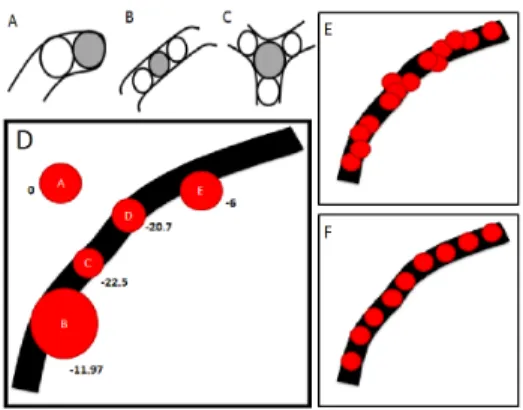
Fig. 2: A,B,C - possible neighborhood spatial configurations of objects. D: High negative data energies indicate ”good” objects. E,F: uniform spacing between objects (F) is desired over crowding and overlap (E) in the configurations.

Fig. 3: Evolution of configurations. Every iteration, at the birth phase objects are added (grey) to the surviving set (green) from the previous iterations with centre and radii independently sampled from image volume and radii range respectively. Objects failing to meet the neuriteness and interaction constraints are removed (red) in the death step. Iterations continue until no more new objects can be added.

1) Fit to data: The data energy checks the fit of the object to the image volume and is based on a tubularity filter proposed in [31]. Eigen analysis at the scale of object radii determines the local width and orientation of branch and the normal plane spanned by the local Hessian eigenvectors V 1 and V 2. The medialness measure M(ωi) is an average of the

gradient response at a scale σGproportional to the object radii

averaged by a rotating phasor Vθ= cos(θ )V1+ sin(θ )V2along

the circumference of the cut of the spherical object on the normal plane: M(ωi) = | π 2 Z_2π θ =0 ∇I(σG)_(x i+ riVθ)dθ |. (6)

An adaptive thresholding of the medialness response Mc(ωi) =

|∇I(σH)_(x

i)| discriminates between “good” and “bad” objects.

Fig. 2D shows the adopted neurite-ness function on 1 slice of data with the cuts of our spherical objects (red). High negative energies indicate “good” objects (eg. objects B,C,D) i.e. spheres situated on the branch centreline and the same size as the local branch width. “Bad” objects, for example, on the background (object A) or not centered correctly on the branch (object E) have low probabilities of survival in the configuration during the energy minimization scheme. The data energy response is then defined as follows:

Ud(ωi) =

(

−(M(ωi) − Mc(ωi)), if M(ωi) > Mc(ωi)

0, otherwise. (7) 2) Connectedness: A pair-wise interaction potential for objects in each other’s zone of influence imposes continuity constraints on the configuration of objects modeling neuronal fibers. In poorly stained, fragmented sections, when the data energy response is not favorable, this term still ensures survival of the object in the configuration to ensure continuity of branches. U is a repulsive potential to penalize overlapping objects, and −U is an attractive potential to favor objects in touching distances of each other. Every object is surrounded by a zone of repulsion where birth of other objects are discouraged to prevent clustering and overlapping of objects. Beyond the zone of repulsion is a concentric zone of attraction where birth of objects are favored to preserve continuity of structures. The following equation illustrates this prior:

Ui(ωi, ωj) =      U, if d < dr −U, if dr≤ d ≤ da 0, if d > da. (8)

Here, d is the Euclidean distance between the centers of the spheres; dr and da (dr < da) are respectively the repulsive

and attractive distances, dr= ri+ rj, da= 2 ∗ dr. By varying

dr and da, density of spheres along the neuronal branches can

be controlled. Refer Fig. 2E,F to see the effect of connection prior on the MPP configurations. We see unevenly spaced con-figuration on the left, considering radiometric properties only. On the right, we see object at uniform distances considering interaction constraints in addition to radiometric properties.

3) Spatial configurations: The second prior is a multi-object interaction potential, incorporating constraints on the local sub-configurations depending on k(ωi) = |ωj∈ γ : dr<

d(ωi, ωj) < da| number of immediate neighbors of an object.

Fig. 2A,B,C highlights the sub configurations that are rou-tinely encountered in axonal structures — A: terminal, B: anchor points along the length of a branch, and C: bifurcation junction. The spatial configuration prior is designed to favor bifurcations and terminals with negative potential E1, to

en-courage survival of such sub-configurations. At the same time, it discourages isolated objects in the configuration, which are

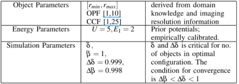
Object Parameters [rmin, rmax]

OPF [1,10] CCF [1,25]

derived from domain knowledge and imaging resolution information Energy Parameters U= 5, E1= 2 Prior potentials;

empirically calibrated. Simulation Parameters δ ,

β = 1, ∆δ = 0.999, ∆β = 0.998

δ and ∆δ is critical for no. of objects in optimal configuration. The condition for convergence is ∆β < ∆δ < 1

TABLE I:Marked point process model parameters. likely to correspond to cell nuclei or other such background structures. It not only provides a sophisticated semantic in-terpretation of neuronal morphology but also generates char-acteristic descriptors for the extracted neurons as mentioned earlier in the introduction. We propose the improved prior as follows: Uc(ωi) =      ∞, if k(ωi) = 0 −E1, if k(ωi) = 1, 3 ∞, if k(ωi) > 3 (9)

C. Sampling and estimation

The goal of the proposed approach is to sample special con-figurations of spherical objects and fit them to the microscopy data stacks to voxels of maximum neuriteness measures. Spherical objects with a 1-dimensional object space limit the computational complexity of sampling and estimation. These configurations are projected onto the image volume and a similarity between the proposed configuration and the neuronal data is computed by a Gibbs energy model defined on the configuration space. The optimum global energy is defined over the space of union of all possible configurations, con-sidering an unknown a-priori number of objects. Exhaustive search of the solution space is impractical. Hence, we choose an efficient Multiple Birth and Death (MBAD) dynamics [10] to find the Maximum A Posteriori (MAP) estimation (Eq.4), greatly reducing computational cost and speeding up convergence. The discretization of the continuous case and its convergence conditions are proved in [10]. We optimize the object configuration in an iterative scheme, where multiple random objects are proposed and removed independently and simultaneously in each iteration depending on the relative energy change due to their introduction. We sample from the probability distribution µβ(γ) using a Markov chain of

the discrete-time MBAD dynamics defined on Ω and apply a Simulated Annealing scheme. At every iteration, a transition is considered from current configuration γ to γ0∪ γ00 where γ0 ⊂ γ and γ00 is any new configuration. The corresponding transition probability is given by:

(10) P(γ → γ0∪ γ00) ∼ (zδ )|γ 00 |

∏

∏

where αβ(ωi, γ) = exp(−β (U(γ \ ωi) − U (γ))). The

conver-gence properties of the Markov Chain to the global minimum under a decreasing scheme of parameters δ and _β1 are proved in [10]. The probability of death of an object depends on both the temperature and its relative energy in the sub-configuration; whereas, birth of object is independent of both energy and temperature and is spatially homogeneous. In this way, the iterative process finds a configuration ˆγ minimizing the global energy Eq. 5.

IV. RECONSTRUCTION

Digital reconstruction of neuronal trees contain position, shape and connection hierarchy of the neuronal branches. The position is reflected by the centreline, which along with local width gives an accurate representation of the branch topology. A graph theoretic model further augments this description with the complex connection pattern of branches and generate a Minimum Spanning Tree(MST) encoding.

In this section, we focus on a tree traversal of the detected MPP objects. We generate a adjacency matrix with the MPP objects as nodes of a graph n1, n2. . . ∈ N, taking the Euclidean distance

between connected nodal pairs as the edge weight. We have sorted the nodes according to Euclidean closeness and allowed objects within attractive distances of each other in the MPP final configurations to be connected. A MST representation of the detected set of objects is derived from the adjacency matrix using Kruskal’s algorithm [18]. Next, the notion of neighbor-ing nodes is augmented by incorporatneighbor-ing image potential on top of Euclidean distance between the centers of MPP objects. This consideration of image data in inferring and verifying the connectivity removes the false positives and is particularly important at the junctions or densely branched zones. For this purpose, first, we adopt a gradient vector field based speed map to guide front propagation, taking into account the anisotropy of the voxels in the image stack. Second, we choose the parameter-free fast marching methods to extract the neuronal fibres as geodesic paths. This framework is presented in [6].Beginning with the root R, a depth first traversal of the obtained MST, by computing the minimal geodesic path between neighboring nodes, gives us the directed MST of the voxels representing the centreline of the neuronal structure. The speed map for aiding Front Propagation (FP) in our algorithm is computed by diffusion of a Gradient Vector Field (GVF) as proposed by Xu. et al in [40]. It enables edge-preserving diffusion of gradient information. The GVF exhibits some characteristic properties in case of tubular structures — the magnitude of the gradient vector decreases in-wards away from the boundary and vanishes at the center. For given image volume I, and an initial vector field F = |∇IσG_|,

where σG is the scale of the gaussian, the GVF is defined as

the vector field V (x) that minimizes the energy:

Egv f(x) =

Z Z Z

V3

µ |∇V (x)|2+|F(x)|2|V (x) − F(x)|2. (11) Here, voxel vector x = (x, y, z) ∈ V3_{, the image domain, and µ}

is a parameter for balancing between the two terms dependent on noise level in data. We calculate the average outward flux for every voxel using the divergence theorem [36]. The divergence at a point is defined as the net outward flux per unit volume, as the volume about the point shrinks to zero:

D(x) = 1 Ni

Z Z Z

V3

V(xi). ˆnidSi. (12)

Here Ni is a 26-neighbor of xi and ˆni is the unit outward

normal at xi of the unit sphere Si in 3D, centered at xi.

Fast Marching methods (FMM) find numerical approximate solutions to the boundary value problems of the Eikonal equation [22]:

F(x)|∇T (x)|= 1. (13) Here T (x) is an arrival time map that denotes the time taken by a front originating from xs and propagating according to

the speed map F(x) to reach voxel xf. We allow the front

to propagate guided by the speed image F(x) until it reaches the target nodes ni from the node list N. A gradient descent

from target node nf ← ni to the start node of marching front

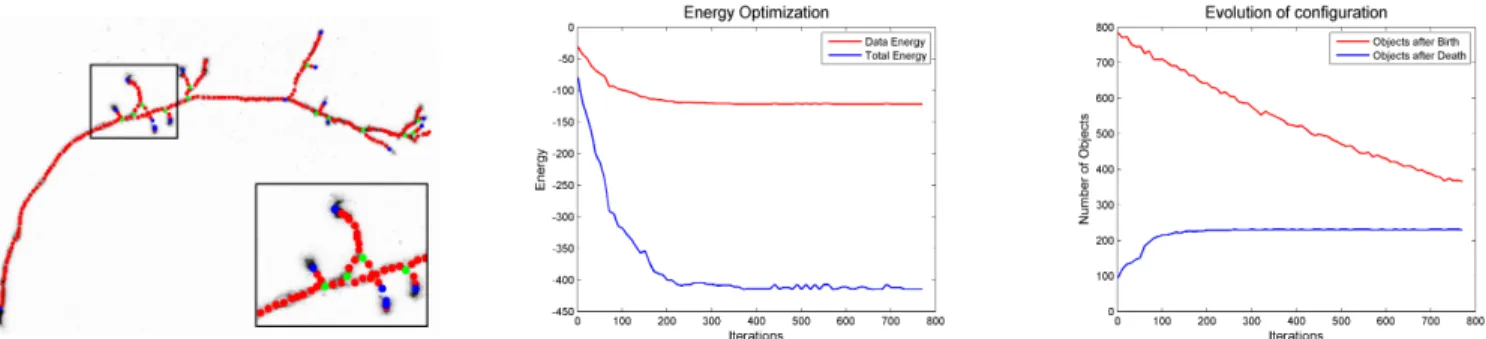
Fig. 4: Neurite branches detected by spherical objects on Olfactory Projection Fibre 7. Corresponding graphs show the convergence of the algorithm in term of number of objects at every iteration: in red is a number of added objects after birth and in blue after death. The energy plots show that at convergence the optimal configuration has a globally minimum energy. δ0= 2400, ∆δ= 0.999,fraction of objects at every

iteration f =1₃, no of iterations n = 780. It took 57 minutes on a Intel Core i7 processor, 2.80GHz and 16 GB RAM.

the arrival time map T (x) extracts the path corresponding to the shortest arrival time between the start node ns← xs

and end node nf ← xf. The resulting minimal path p is

updated to the list of minimal paths pi∪ p. Next, we make

target node our new start node ns← ni, remove it from node

list N = N − ni and re-initialize the front to extract the next

part of the neuron tree. When the gradient descent fails to reach the start node, we remove the target/end node as a false detection. The algorithm terminates when node list N is empty. In this way, FMM captures accurate minimum spanning tree representation of neuronal morphology by iteratively adding minimal paths between nodes [9]. FFM offers several desirable features such as inherent connectivity and smoothness, which counteract noise and cross-section irregularities.

V. EXPERIMENTS AND RESULTS

We tested our proposed model on 3D light microscopy image stacks featured in the DIADEM challenge [7], which represent some of the most challenging and diverse neuron morphology to try the computational intelligence of automated tracing algorithms. From the database, we choose the data sets representing single neuron image stacks. The task of separating fibres from multiple sources is better resolved at the experimental stage as demonstrated by the Brainbow technique in [19]. The Olfactory Projection Fibre axons are acquired by 2-channel confocal microscopy and the Cerebellar Climbing Fibres are acquired by transmitted light brightfield microscopy. For both types of neurons we have several datasets representing their natural morphological variation.

In Table. I, we list the parameters of the algorithm and explain how they are initialized. Our analysis revealed that only the parameters radius range [rmin, rmax] and the birth

intensity δ are data dependent. The model is sensitive to the initialization of the birth intensity, which is generally set as an over estimation of the expected number of objects in the final configuration. We propose simple rules to automatically estimate the birth intensity initialization, to free the users from the burden of tuning them manually for each new data set. Binary clustering into foreground and background gives an approximate volume of neurites P. Let f (I) be the number of objects expected from the radiometric term. This can be

approximated as f (I) = P

4πr3_m 3

, where rm is the mean radius.

Our unoptimized Matlab implementation takes on average 57 mins and 1hr 33 mins to converge on OPF and CCF data sets respectively, on a PC running Intel Core i7 processor, 2.80GHz and 16 GB RAM.

The validation of traces is a topic of much research with

gFN gFP cFN cFP

MPP 0.026±0.005 0.042±0.006 0.35±0.17 0.44±0.20 MPP+FFM 0.026±0.005 0.042±0.006 0.327±0.12 0.282±0.12

TABLE II: NetMets scores for MPP+FFM.

OP1 OP4 OP5 OP6 OP7 OP8 overall

δ0 2150 1850 1000 1350 1100 1100 No. of objects in final configuration 435 358 204 283 226 223 DIADEM Score MPP 0.829 0.789 0.797 0.830 0.921 0.854 0.837±0.043 DIADEM Score MPP+FFM 0.846 0.807 0.818 0.854 0.926 0.863 0.852±0.038

TABLE III:DIADEM scores

Avg Manual Tracer[26] M 0.78±0.1 Stepanyants et. al[8] SA 0.80±0.1 Wang et. al [37] SA 0.863 Mukerjee et. al[26] A 0.82±0.07

Xiao et. al[39] A 0.77±0.17 MPP A 0.837±0.043 MPP+FFM A 0.852±0.038

TABLE IV: DIADEM scores comparison. M-Manual; SA-Semi-Automatic; A-Automatic. SNT (SA)[21] Neurolucida (SA)[16] 3Dtip (A)[20] APP2 (A)[39] MPP(A) OP1 41 49 48 43 43 OP4 43 61 46 46 39 OP5 9 9 17 6 9 OP6 18 18 23 12 16

TABLE V: Terminals on various data sets using various tracing tools. SA-Semi-Automatic; A-Automatic.

various metrics being employed [13], [15], [24]. We evaluate our automatic reconstruction using the standard DIADEM metric [14] and the newly proposed NetMets metric [23], [24].

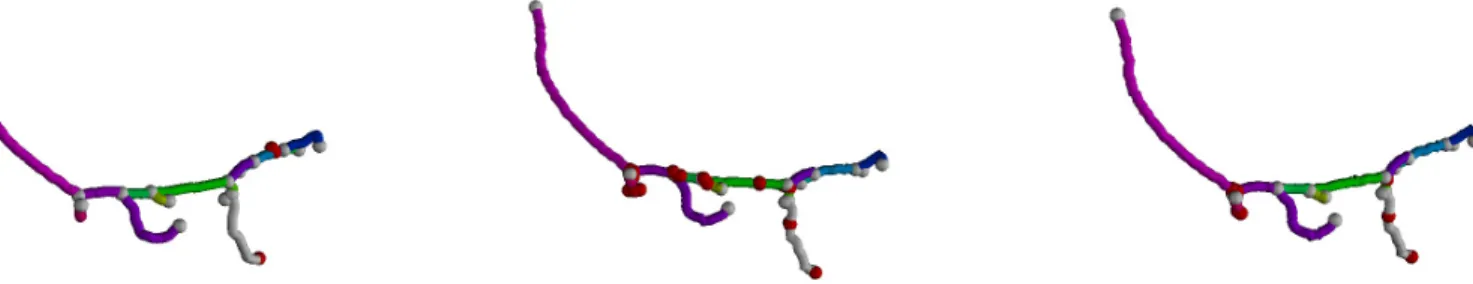
Fig. 5:(a) Gold standard reconstruction (b) MPP reconstruction (c) MPP+FFM reconstruction. The red nodes indicate the erroneous regions. The FFM based reconstruction further improves the reconstruction from the MPP configurations.

Fig. 6:MPP configuration Fig. 7:Reconstructed MST

Fig. 8:Visualization of obtained terminals (blue) and branching nodes (green) by various tracing methods.

The NetMets software is a general graph comparison tool with an expressive scoring system for the quantification and visualization of errors in two biological networks. It scores the geometric (g) and connectivity (c) false positive (FP) and false negative (FN) rates gFN, gFP, cFN, cFP. It helps us to quantify and visualize how the incorporation of an image potential in inferring connectedness of nodes reduces false positive rates and improves overall reconstruction. Refer to NetMets generated graphs (Fig. 5) for visualization of reconstructions with MPP and MPP+FFM against the manual gold standard (Fig. 5a). Red node indicates the missed branches. Fig. 5(b) shows the automatic reconstruction with our proposed marked point process. Red nodes indicate the false positive nodes. Figure 5(c) shows reconstruction using fast marching and marked point process, where we can see false positive nodes are removed. Figs. 6 and 7 show respectively the detection by our MPP model and reconstruction by our proposed pipeline on the Cerebellar Climbing Fibres.

The DIADEM metric gives a combined F-score for the posi-tion and connecposi-tion of the reconstructed neuron by comparing against a manual gold standard reconstruction. The DIADEM metric is particularly crafted for scoring tree hierarchic neu-ronal reconstructions and is relaxed in penalizing errors far from the root node. In Table. IV, is presented the DIADEM metric scores of various reconstruction tools. The existing methods are mostly interactive or semi-automatic and incor-porate user-interaction at some stage of reconstruction. The Open Snake based method [37] and the method presented by Stepanyants et. al [8] were judged the two best methods in the DIADEM challenge. But with the Open Snake method there is significantly large variance, 0.863 ± 0.35, due to

incorpo-ration of user interaction for proof-editing and optimization of initial automatic trace. We observe that our MPP+FFM framework improves overall accuracy of automated neurite tracing and minimizes variability with a DIADEM metric score of 0.852 ± 0.038.

In our experience with various semi-automatic tools for neu-ronal morphometry analysis, the baseline inter operator vari-ability limits DIADEM metric score at 0.91. Indeed, this repre-sents the inherent limitation of validation against gold standard manual reconstructions due to lack of a singular ground truth. Table. V lists the different number of terminal nodes obtained on the same data using different tracing tools. In Fig. 8, we highlight some of the erroneous interpretation of neuronal morphology by these softwares. For example, Fig. 8(A) shows the tracing by Vaa3D has obtained terminal points at points of high curvature along neuronal branches. Fig. 8(B) shows the tracing by Neurolucida resolves branch terminals presenting a blob-like appearance as a bifurcation node with two short tiny branches. Our model is not sensitive to the complex variability of branch morphology presented by neurites Fig. 8(C). It resolves blob-like terminals correctly with fitting a bigger sphere instead of interpreting as a branching point with two short branches. Similarly, points of branch curvature are correctly identified as inflection point and not terminals. Our proposed model thus provides more sophisticated and accurate semantic interpretation of neuronal morphology compared to existing tools.

VI. CONCLUSION

We propose a novel marked point process approach to detect complex neuronal morphology as the global optimum of a well designed energy function. Unlike existing methods, it models neuronal trees with sophisticated semantic priors generating

geometric and morphological features to characterise neuronal morphology. Our neurite tracing pipeline incorporates image potential in inferring connectedness of neuronal nodes without greatly increasing computational cost. We have presented a fully automatic framework combining marked point process neurite model and fast marching for digital reconstruction of 3D neuronal morphology. Our proposed method outperforms the existing automatic tracing algorithms and minimizes the variability of interactive tracing.

REFERENCES

[1] SR Aylward and E Bullitt. Initialization, noise, singularities and scale in height ridge traversal for tubular object centerline extraction. IEEE Transactions on Medical Imaging, 21(2):61–75, 2002.

[2] AJ Baddeley and MNM Van Lieshout. Stochastic geometry models in high-level vision. Journal of Applied Statistics, 20(5-6):231–256, 1993. [3] S Basu, A Aksel, B Condron, and ST Acton. Tree2tree: neuron segmentation for generation of neuronal morphology. In Proceedings of IEEE International Symposium on Biomedical Imaging,(ISBI), pages 548–551, 2010.

[4] S Basu, MS Kulikova, E Zhizhina, WT Ooi, and D Racoceanu. A stochastic model for automatic extraction of 3d neuronal morphology. Proceedings of International Conference on Medical Image Computing and Computer Assisted Intervention (1), (MICCAI), pages 396–403, 2013.

[5] S Basu, WT Ooi, and D Racoceanu. Improved marked point process priors for single neurite tracing. Proceedings of International Workshop on Pattern Recognition in Neuroimaging, (PRNI), pages 1–4, 2014. [6] S Basu and D Racoceanu. Reconstructing neuronal morphology from

microscopy stacks using fast marching. Proceedings of IEEE Interna-tional Conference on Image Processing, (ICIP), pages 3597 – 3601, October 2014.

[7] KM Brown, G Barrionuevo, AJ Canty, V De Paola, JA Hirsch, GSXE Jefferis, J Lu, M Snippe, I Sugihara, and GA Ascoli. The diadem data sets: Representative light microscopy images of neuronal morphology to advance automation of digital reconstructions. Neuroinformatics, pages 1–15, 2011.

[8] P Chothani, V Mehta, and A Stepanyants. Automated tracing of neurites from light microscopy stacks of images. Neuroinformatics, 9(2-3):263– 278, 2011.

[9] LD Cohen and R Kimmel. Fast marching the global minimum of active contours. Proceedings of IEEE International Conference on Image Processing (1),(ICIP), pages 473–476, 1996.

[10] X Descombes, R Minlos, and E Zhizhina. Object extraction using a stochastic birth-and-death dynamics in continuum. Journal of Mathe-matical Imaging and Vision, 33(3):347–359, 2009.

[11] DE Donohue and GA Ascoli. Automated reconstruction of neuronal morphology: An overview. Brain Research Reviews, 67:94 – 102, 2011. [12] AF Frangi, WJ Niessen, KL Vincken, and MA Viergever. Muliscale vessel enhancement filtering. Proceedings of International Conference on Medical Image Computing and Computer Assisted Intervention (1), (MICCAI), pages 130–137, 1998.

[13] R Gala, J Chapeton, J Jitesh, C Bhavsar, and A Stepanyants. Active learning of neuron morphology for accurate automated tracing of neu-rites. Frontiers in Neuroanatomy, 8, 2014.

[14] TA Gillette, KM. Brown, and GA Ascoli. The diadem metric: Com-paring multiple reconstructions of the same neuron. Neuroinformatics, 9(2-3):233–245, 2011.

[15] TA Gillette, KM Brown, K Svoboda, Y Liu, and GA Ascoli. Di-ademchallenge.org: A compendium of resources fostering the continuous development of automated neuronal reconstruction. Neuroinformatics, 9(2-3):303–304, 2011.

[16] M Halavi, KA Hamilton, R Parekh, and GA Ascoli. Digital recon-structions of neuronal morphology: three decades of research trends. Frontiers in neuroscience, 6, 2012.

[17] K Krissian, G Malandain, N Ayache, R Vaillant, and Y Trousset. Model-based multiscale detection of 3d vessels. Proceedings of IEEE Conference on Computer Vision and Pattern Recognition, (CVPR), pages 722–727, 1998.

[18] JB Kruskal. On the shortest spanning subtree of a graph and the traveling salesman problem. Proceedings of the American Mathematical Society, pages 48–50, 1956.

[19] JW Lichtman, J Livet, and JR Sanes. A technicolour approach to the connectome. Nature Reviews Neuroscience, 9(6):417–422, 2008.

[20] M Liu, HPeng, AK Roy Chowdhury, and EW Myers. 3d neuron tip detection in volumetric microscopy images. Proceedings of IEEE International Conference on Bioinformatics and Biomedicine, (BIBM), pages 366–371, 2011.

[21] MH Longair, DA Baker, and JD Armstrong. Simple neurite tracer: open source software for reconstruction, visualization and analysis of neuronal processes. Bioinformatics, 27(17):2453–2454, 2011.

[22] R Malladi and JA Sethian. Level set and fast marching methods in image processing and computer vision. Proceedings of IEEE International Conference on Image Processing (1),(ICIP), pages 489–492, 1996. [23] D Mayerich, C Bj¨ornsson, J Taylor, and B Roysam. Metrics for

com-paring explicit representations of interconnected biological networks. Proceedings of Symposium on Biological Data Visualization, (BioVis), pages 79–86, 2011.

[24] D Mayerich, C Bjornsson, J Taylor, and B Roysam. Netmets: software for quantifying and visualizing errors in biological network segmenta-tion. BMC Bioinformatics, 13(Suppl 8):S7, 2012.

[25] E Meijering. Neuron tracing in perspective. Cytometry Part A, 77(7):693–704, 2010.

[26] A Mukherjee and A Stepanyants. Automated reconstruction of neural trees using front re-initialization. In Proceedings of SPIE Medical Imaging, pages 83141I–83141I. International Society for Optics and Photonics, 2012.

[27] S Mukherjee and ST Acton. Vector field convolution medialness applied to neuron tracing. Proceedings of IEEE International Conference on Image Processing, (ICIP), pages 665–669, 2013.

[28] S Mukherjee, B Condron, and ST Acton. Neuron segmentation with level sets. In Proceedings of Asilomar Conference on Signals, Systems and Computers, pages 1078–1082. IEEE, 2013.

[29] H Peng, F Long, and G Myers. Automatic 3d neuron tracing using all-path pruning. Bioinformatics [ISMB/ECCB], 27(13):239–247, 2011. [30] H Peng, Z Ruan, D Atasoy, and S Sternson. Automatic reconstruction of 3d neuron structures using a graph-augmented deformable model. Bioinformatics, 26(12):i38–i46, 2010.

[31] T Pock, C Janko, R Beichel, and H Bischof. Multiscale medialness for robust segmentation of 3d tubular structures. Proceedings of the Computer Vision Winter Workshop, pages 93–102, 2005.

[32] R Rigamonti and V Lepetit. Accurate and efficient linear structure seg-mentation by leveraging ad hoc features with learned filters. Proceedings of International Conference on Medical Image Computing and Computer Assisted Intervention (1), (MICCAI), pages 189–197, 2012.

[33] SL Senft. A brief history of neuronal reconstruction. Neuroinformatics, 9(2):119–128, 2011.

[34] A Sironi, V Lepetit, and P Fua. Multiscale centerline detection by learning a scale-space distance transform. In Computer Vision and Pattern Recognition (CVPR), Proceedings of IEEE Conference on, pages 2697–2704. IEEE, 2014.

[35] E T¨uretken, G Gonz´alez, C Blum, and P Fua. Automated reconstruction of dendritic and axonal trees by global optimization with geometric priors. Neuroinformatics, 9(2-3):279–302, 2011.

[36] A Vasilevskiy and K Siddiqi. Flux maximizing geometric flows. IEEE Transactions on Pattern Analysis and Machine Intelligence, 24(12):1565–1578, 2002.

[37] Y Wang, A Narayanaswamy, CL Tsai, and B Roysam. A broadly applicable 3-d neuron tracing method based on open-curve snake. Neuroinformatics, 9(2-3):193–217, 2011.

[38] JG White, E Southgate, JN Thomson, and S Brenner. The structure of the nervous system of the nematode caenorhabditis elegans. Philosophical Transactions of the Royal Society of London. Series B, Biological Sciences, 314(1165):1–340, 1986.

[39] H Xiao and H Peng. App2: automatic tracing of 3d neuron morphology based on hierarchical pruning of a gray-weighted image distance-tree. Bioinformatics, 29(11):1448–1454, 2013.

[40] C Xu and JL Prince. Snakes, shapes, and gradient vector flow. IEEE Transactions on Image Processing, 7(3):359–369, 1998.

[41] J Yang, PT Gonzalez-Bellido, and H Peng. A distance-field based automatic neuron tracing method. BMC Bioinformatics, 14:93, 2013. [42] T Zhao, J Xie, F Amat, N Clack, P Ahammad, H Peng, F Long, and

E Myers. Automated reconstruction of neuronal morphology based on local geometrical and global structural models. Neuroinformatics, 9(2-3):247–261, 2011.