HAL Id: tel-01725363
https://tel.archives-ouvertes.fr/tel-01725363
Submitted on 7 Mar 2018HAL is a multi-disciplinary open access archive for the deposit and dissemination of sci-entific research documents, whether they are pub-lished or not. The documents may come from teaching and research institutions in France or abroad, or from public or private research centers.
L’archive ouverte pluridisciplinaire HAL, est destinée au dépôt et à la diffusion de documents scientifiques de niveau recherche, publiés ou non, émanant des établissements d’enseignement et de recherche français ou étrangers, des laboratoires publics ou privés.
Shaifali Parashar
To cite this version:
Shaifali Parashar. Image-based Deformable 3D Reconstruction using Differential Geometry and Car-tan’s Connections. Computer Vision and Pattern Recognition [cs.CV]. Université Clermont Auvergne, 2017. English. �tel-01725363�
Ann´ee Nod’ordre
ECOLE DOCTORALE
DES SCIENCES POUR L’INGENIEUR
TH`
ESE
Pr´esent´ee `a l’Universit´e Clermont Auvergne
pour l’obtention du grade de DOCTEUR (D´ecret du 5 juillet 1984) Specialit´e COMPUTER VISION Soutenue le 23 Novembre 2017
Shaifali Parashar
Image-based Deformable 3D Reconstruction
using Differential Geometry
and Cartan’s Connections
Pr´esidente Marie-Odile Berger, Research Director, INRIA-Nancy, France
Rapporteurs Mathieu Salzmann, Researcher, EPFL, Switzerland
Alessio Del Bue, Researcher, IIT-Genova, Italy
Directeur de th`ese Adrien Bartoli, Professor, Universit´e Clermont Auvergne, France
Co-encadrant Daniel Pizarro, Lecturer, Universidad de Alcal´a, Spain
EnCoV, Institut Pascal, UMR 6602 CNRS, Universit´e Clermont Auvergne, SIGMA
Facult´e de M´edecine
28 Place Henri Dunant, Clermont-Ferrand Tel: +33 4 73 17 81 23
Acknowledgements
I would like to express my gratitude to my supervisors Adrien and Dani who always inspired and guided me during my PhD. With their immense knowledge about the field, they helped me a lot in looking for the right answers which led to my research. I am very thankful for their kindness, patience and a friendly assistance. I highly appreciate the fact that Adrien has always been available for a discussion. I am very grateful to Dani for his support. I have always found him insightful and his contributions are very significant in the development of this thesis. Both of them have been very friendly and caring, which has made this PhD a great learning experience for me.
I would also like to thank Toby for his guidance. His knowledge and perspective about research has helped me a lot in my research. It was a great pleasure to have spent time in this lab where everyone is so friendly and helpful. I have learnt a great deal from all of them and I will always cherish the memories of this time spent together.
In addition, I would like to thank the thesis jury reporters, Mathieu Salzmann and Alessio Del Bue for carefully reading the document and providing constructive remarks that has provided further encouragement to me for research in the field. I would also like to thank Marie-Odile Berger for her role of the President of the jury and her valuable comments.
I am also thankful to my parents and Alok for their unconditional love which helped a lot during these PhD years.
Abstract
Reconstructing the 3D shape of objects from multiple images is an important goal in computer vision and has been extensively studied for both rigid and non-rigid (or deformable) objects. Structure-from-Motion (SfM) is an algorithm that performs the 3D reconstruction of rigid objects using the inter-image visual motion from multiple images obtained from a moving camera. SfM is a very accurate and stable solution. Deformable 3D reconstruction, however, has been widely studied for monocular images (obtained from a single camera) and still remains an open research problem. The current methods exploit visual cues such as the inter-image visual motion and shading in order to formalise a reconstruction algorithm. This thesis focuses on the use of the inter-image visual motion for solving this problem. Two types of scenarios exist in the literature: 1) Non-Rigid Structure-from-Motion (NRSfM) and 2) Shape-from-Template (SfT). The goal of NRSfM is to reconstruct multiple shapes of a deformable object as viewed in multiple images while SfT (also referred to as template-based reconstruction) uses a single image of a deformed object and its 3D template (a textured 3D shape of the object in one configuration) to recover the deformed shape of the object.
We propose an NRSfM method to reconstruct the deformable surfaces undergoing iso-metric deformations (the objects do not stretch or shrink under an isoiso-metric deformation) using Riemannian geometry. This allows NRSfM to be expressed in terms of Partial Differ-ential Equations (PDE) and to be solved algebraically. We show that the problem has linear complexity and the reconstruction algorithm has a very low computational cost compared to existing NRSfM methods. This work motivated us to use differential geometry and Cartan’s theory of connections to model NRSfM, which led to the possibility of extending the solution to deformations other than isometry. In fact, this led to a unified theoretical framework for modelling and solving both NRSfM and SfT for various types of deformations. In addition, it also makes it possible to have a solution to SfT which does not require an explicit modelling of deformation. An important point is that most of the NRSfM and SfT methods reconstruct the thin-shell surface of the object. The reconstruction of the entire volume (the thin-shell surface and the interior) has not been explored yet. We propose the first SfT method that reconstructs the entire volume of a deformable object.
Resum´e
La reconstruction 3D d’objets `a partir de plusieurs images est un objectif important de la vision par ordinateur. Elle a ´et´e largement ´etudi´ee pour les objets rigides et non rigides (ou d´eformables). Le Structure-from-Motion (SfM) est un algorithme qui effectue la reconstruc-tion 3D d’objets rigides en utilisant le mouvement visuel entre plusieurs images obtenues `a l’aide d’une cam´era en mouvement. Le SfM est une solution tr`es pr´ecise et stable. La recon-struction 3D d´eformable a ´et´e largement ´etudi´ee pour les images monoculaires (obtenues `a partir d’une seule cam´era) mais reste un probl`eme ouvert. Les m´ethodes actuelles exploitent des indices visuels tels que le mouvement visuel inter-image et l’ombrage afin de construire un algorithme de reconstruction. Cette th`ese se concentre sur l’utilisation du mouvement visuel inter-image pour r´esoudre ce probl`eme. Deux types de sc´enarios existent dans la litt´erature: 1) le Non-Rigid Structure-from-Motion (NRSfM) et 2) le Shape-from-Template (SfT). L’objectif du NRSfM est de reconstruire plusieurs formes d’un objet d´eformable tel qu’il apparaˆıt dans plusieurs images, alors que le SfT (´egalement appel´e reconstruction `a partir d’un mod`ele de r´ef´erence) utilise une seule image d’un objet d´eform´e et son mod`ele 3D de r´ef´erence (une forme 3D textur´ee de l’objet dans une configuration) pour estimer la forme d´eform´ee de l’objet.
Nous proposons une m´ethode de NRSfM pour reconstruire les surfaces d´eformables soumises `a des d´eformations isom´etriques (les objets ne s’´etirent pas ou ne se contractent pas sous une d´eformation isom´etrique) en utilisant la g´eom´etrie riemannienne. Cela per-met d’exprimer le NRSfM en termes d’´equations aux d´eriv´ees partielles et de le r´esoudre alg´ebriquement. Nous montrons que le probl`eme a une complexit´e lin´eaire et que l’algorithme de reconstruction propos´e a un coˆut de calcul tr`es bas compar´e aux m´ethodes existantes de NRSfM. Ce travail nous a motiv´e `a utiliser la g´eom´etrie diff´erentielle et la th´eorie des con-nexions de Cartan pour mod´eliser le NRSfM, ce qui nous a permis d’´etendre la solution `a des d´eformations autres que l’isom´etrie. En fait, cela a conduit `a un cadre th´eorique unifi´e pour mod´eliser et r´esoudre le NRSfM et le SfT pour diff´erents types de d´eformations. Ce cadre permet ´egalement d’avoir une solution au SfT qui ne n´ecessite pas de mod´elisation explicite de la d´eformation. Un point important est que la plupart des m´ethodes de NRSfM et de SfT reconstruisent la surface de l’objet (hypoth`ese coque mince). La reconstruction de l’ensemble d’un volume (la surface et l’int´erieur d’un objet) n’avait pas encore ´et´e explor´ee. Nous proposons la premi`ere m´ethode de SfT qui reconstruit le volume complet d’un objet d´eformable.
Contents
Abstract vii
Resum´e ix
1 Introduction 1
1.1 Background . . . 1
1.2 3D Reconstruction of Deformable Objects . . . 4
1.2.1 Shape-from-Template . . . 4 1.2.2 Non-Rigid Structure-from-Motion. . . 4 1.2.3 Current Limitations . . . 5 1.3 Contributions . . . 5 2 Related Work 13 2.1 Shape-from-Template. . . 13
2.1.1 Thin-Shell Initialisation Methods . . . 14
2.1.2 Thin-Shell Refinement Methods. . . 16
2.1.3 Shape-from-Template for Volumetric Objects . . . 18
2.1.4 Relationship to our Work . . . 18
2.2 Non-Rigid Structure-from-Motion. . . 19
2.2.1 Methods with Statistics-based Models . . . 19
2.2.2 Methods with Physics-based Models . . . 22
2.2.3 Relationship to our Work . . . 23
3 Mathematical Formulation 25 3.1 Notation . . . 25
3.2 Manifolds and Surfaces. . . 26
3.2.1 Infinitesimal Planarity . . . 26
3.2.2 Infinitesimal Linearity . . . 26
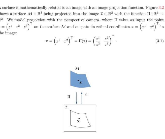
3.3 Projection . . . 27
4 Non-Rigid Structure-from-Motion with Riemannian Geometry 29
4.1 Introduction. . . 30
4.2 Mathematical Background . . . 30
4.2.1 General Model . . . 30
4.2.2 The Metric Tensor. . . 31
4.2.3 Christoffel Symbols. . . 32
4.2.4 Commutativity under Isometry . . . 34
4.2.5 Infinitesimal Planarity . . . 36
4.3 Reconstruction Equations . . . 38
4.3.1 Relating the Metric Tensor and the Christoffel Symbols . . . 39
4.3.2 Solving for the First-Order Derivatives . . . 40
4.3.3 Solving for the Second-Order Derivatives . . . 42
4.4 Algorithms . . . 44
4.4.1 Solution under Infinitesimal Planarity . . . 44
4.4.2 General Solution . . . 44 4.4.3 Complexity Analysis . . . 45 4.5 Experimental Results. . . 45 4.5.1 Synthetic Datasets . . . 46 4.5.2 Real Datasets . . . 49 4.5.3 Elastic Objects . . . 55
4.5.4 Computation Time Comparison. . . 55
4.5.5 Nearly-Stationary Objects . . . 56
4.6 Conclusions . . . 57
5 A Modelling Framework for Deformable 3D Reconstruction 59 5.1 Introduction. . . 60
5.2 Mathematical Background . . . 60
5.2.1 Affine Connections . . . 61
5.2.2 Moving Frames on Surfaces . . . 61
5.2.3 Moving Frames and Parametrisations . . . 64
5.2.4 Smooth Mappings between Surfaces . . . 66
5.2.5 Infinitesimally Linear Mappings between Surfaces. . . 69
5.3 Model-Based 3D Reconstruction . . . 70
5.3.1 Reconstruction Equations for Smooth Mappings . . . 72
5.3.2 Reconstruction Equations for Infinitesimally Linear Mappings . . . 76
5.3.3 Reconstruction Algorithm . . . 77
5.4 Model-Free 3D Reconstruction . . . 78
5.4.1 Reconstruction Equations . . . 79
5.4.2 Reconstruction Algorithm . . . 80
5.5 Experiments and Discussion . . . 81
CONTENTS xiii 5.5.2 Real Datasets . . . 86 5.5.3 Summary of Experiments . . . 94 5.6 Conclusions . . . 94 6 Volumetric Shape-from-Template 95 6.1 Introduction. . . 96 6.2 Mathematical Modelling . . . 96 6.2.1 Geometric Model . . . 96 6.2.2 Deformation Model. . . 98 6.3 Volumetric Shape-from-Template . . . 98
6.3.1 Formulation and Non-Convex Solution . . . 98
6.3.2 Convex Initialisation . . . 99 6.4 Experimental Results. . . 101 6.4.1 Synthetic Datasets . . . 101 6.4.2 Real Datasets . . . 104 6.5 Conclusions . . . 107 7 Conclusions 109 7.1 Thin-Shell Deformable 3D Reconstruction . . . 109
7.2 Volumetric Deformable 3D Reconstruction . . . 110
Appendices 111
A The Metric Tensor 113
B Christoffel Symbols 115
C Differential K-forms 117
List of Figures
1.1 3D reconstruction methods. . . 2
1.2 Some applications of the deformable 3D reconstruction methods. . . 3
1.3 Contribution 1 . . . 7
1.4 Contribution 2 . . . 9
1.5 Contribution 3 . . . 11
1.6 Reconstruction of object’s interior . . . 12
2.1 Surface deformation . . . 14
2.2 Maximum Depth Heuristics formulation . . . 15
3.1 Illustration of Infinitesimal Linearity . . . 27
3.2 Image projection . . . 27
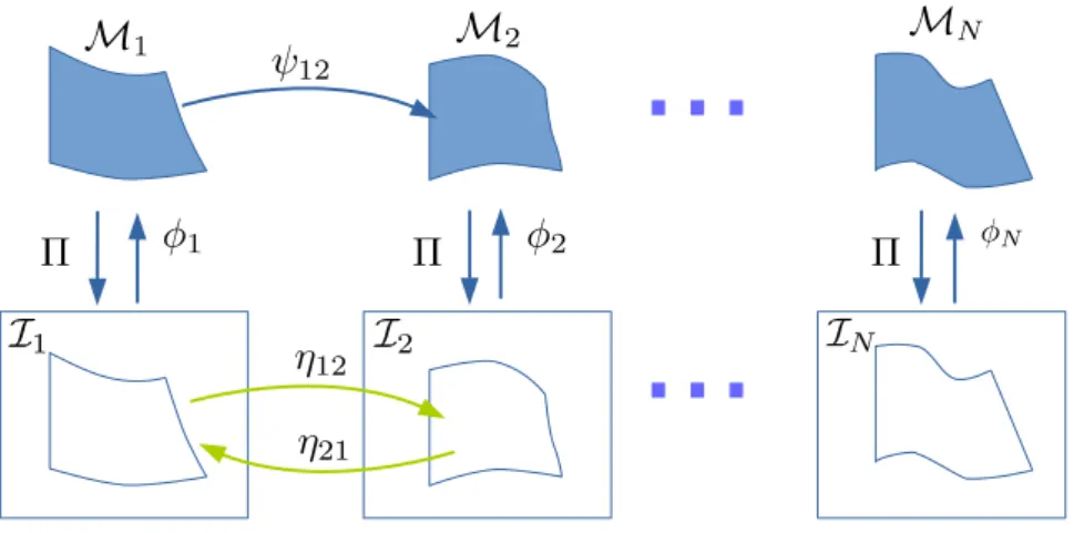
4.1 Proposed model of Non-Rigid Structure-from-Motion . . . 31
4.2 Simplified notation for two images. . . 31
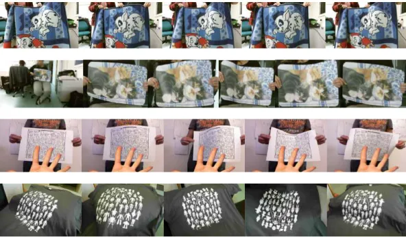
4.3 Some images of the rug, table mat, kinect paper and tshirt datasets . . . 46
4.4 Synthetic data experiments . . . 47
4.5 Experiments on short sequences. . . 50
4.6 Reconstruction error maps and renderings.. . . 52
4.7 Experiments on long sequences . . . 53
4.8 Some images of rubber dataset . . . 54
4.9 Experiment with an almost stationary object . . . 56
5.1 A moving frame. . . 62
5.2 A moving frame under different parametrisations . . . 64
5.3 Surfaces related by a common parametrisation . . . 65
5.4 Classification of various types of smooth mappings. . . 66
5.5 An example of skewless deformation . . . 68
5.6 Modelling of model-based deformable 3D reconstruction . . . 70
5.7 Modelling of model-free deformable 3D reconstruction . . . 78
5.9 Summary of experiments. . . 83
5.10 Performance of compared methods under noisy conditions . . . 85
5.11 Performance of methods on varying curvature . . . 87
5.12 Reconstruction error maps of rubber dataset . . . 88
5.13 Reconstruction error maps of paper dataset . . . 90
5.14 Reconstruction error maps of balloon dataset . . . 91
5.15 Reconstruction error maps of sock dataset . . . 92
5.16 Reconstruction error maps of tissue dataset . . . 93
6.1 Modelling of volumetric Shape-from-Template . . . 97
6.2 Volume interpolation using Local Rigidity. . . 100
6.3 Synthetic data experiments . . . 102
6.4 Results on the woggle dataset . . . 103
6.5 Results on the sponge dataset . . . 104
6.6 Results on the arm dataset . . . 106
6.7 Failure case of volumetric Shape-from-Template . . . 107
List of Tables
2.1 Summary of statistics-based Non-Rigid Structure-from-Motion methods . . . 22
2.2 Summary of physics-based Non-Rigid Structure-from-Motion methods . . . . 24
4.1 Performance of warps in noisy conditions . . . 48
4.2 Summary of experiments on long sequences . . . 54
4.3 Experiment on rubber dataset. . . 55
4.4 Comparison of computation time . . . 56
5.1 Summary of model-based 3D reconstruction of deformable thin-shell objects . 78 5.2 Summary of model-free 3D reconstruction of deformable thin-shell objects . . 80
LIST OF TABLES xix
List of Abbreviations
ARAP As-Rigid-As-PossibleCS Christoffel Symbols
DCT Discrete Cosine Transformation
GS Global Smoothness
IL Infinitesimal Linearity
IP Infinitesimal Planarity
LLS Linear Least Squares
LR Local Rigidity
MDH Maximum Depth Heuristics
NRSfM Non-Rigid Structure-from-Motion
PDE Partial Differential Equations
RMSE Root Mean Square Error
SfM Structure-from-Motion
SfT Shape-from-Template
SIFT Scale Invariant Feature Transform
SOCP Second-order Cone Program
SVD Singular Value Decomposition
TPS Thin-Plate Splines
Chapter
1
Introduction
1.1
Background
An important task in 3D computer vision is to recover 3D information from 2D images obtained by the camera. This task is widely termed as 3D reconstruction. Although there are active image sensors such as the Kinect and Time-of-Flight (ToF) cameras available which can obtain the depth of the view under consideration, passive 3D reconstruction from images remains an interesting topic for researchers because the scope of 3D sensors is limited due to the various constraints of size, cost and accuracy. 3D reconstruction methods rely on various visual cues from images (such as shading, texture, silhouettes, contours and motion) in order to find 3D descriptors such as the depth map and local surface orientation (or normals) of the objects.
The objects found in nature can be roughly classified into rigid or non-rigid (or de-formable) objects. The 3D reconstruction of rigid objects using motion cues, also known as Structure-from-Motion (SfM) [Hartley and Zisserman, 2000] (see figure 1.1a), has been widely studied for the past few decades and there are solutions available which are stable and accurate. SfMexploits the inter-image visual motion information in order to reconstruct 3D from multiple 2D images taken from different views of a rigid object. Rigidity allows the inter-image visual motion to be expressed in terms of the rotation and translation of the camera coordinate frames of the images. However, SfM cannot be extended to deformable objects as between any two images, the deformable object may undergo a deformation and therefore, the inter-image visual motion cannot be expressed only in terms of the camera rotation and translation.
In the past decade, the deformable 3D reconstruction problem has been studied exten-sively in over a hundred research papers. Some of the methods combine motion with other visual cues to disambiguate the problem and make it well-posed. For example, [Liu-Yin et al., 2016; Moreno-Noguer et al., 2009; Varol et al., 2012b] combine shading with motion, [ Gal-lardo et al.,2016,2017] combine shading and contours with motion and [Choe and Kashyap, 1991; White and Forsyth, 2006] combine shading with texture. However, the existing
solu-tions are not close toSfM in terms of accuracy and stability. Deformable 3D reconstruction is an important problem to solve as it has a wide range of applications such as in the medical, sports, entertainment and advertising domains. Some applications are explored in augmented reality: 1) [Smith et al.,2016] shows how to study the impact of a soft ball on various sur-faces. This is useful in designing and testing sports equipments. 2) [Haouchine et al.,2013, 2016; Koo et al., 2017; Maier-Hein et al., 2014] show how to augment the deformations of the body organs in order to aid minimally invasive medical surgeries. 3) [Collins and Bar-toli,2015;Ngo et al.,2015] recover the deformation of the objects in real-time which can be useful in various industries. For example, they can be used by online shopping companies to enable the customers to try clothes and accessories virtually. Figure1.2shows some of these applications. Template SfM Images NRSfM 3D Shape 3D Shape SfT Image +
a) 3D reconstruction of rigid objects
b) 3D reconstruction of non-rigid objects
Figure 1.1: 3D reconstruction methods. For rigid objects, SfM is a widely used method (Images taken from [Snavely et al.,2007]). The 3D reconstruction of deformable objects can be performed by either NRSfMor SfTmethods.
This thesis focuses on the monocular deformable 3D reconstruction methods that use motion as a visual cue in monocular imaging conditions. We now define the problem in detail and describe our contributions.
1.1. BACKGROUND 3
a) [Collins et al., 2015] shows an application for real-time SfT. The deformations of an object viewed in a single image can be transformed to other objects.
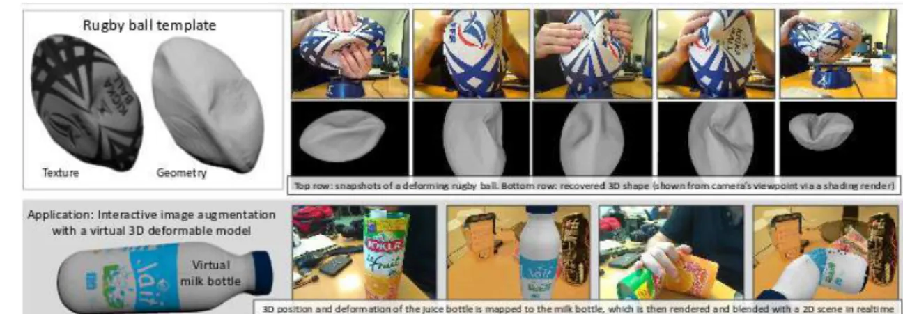
b) [Smith et al., 2016] shows an application for SfT. The reconstructed deformed ball can be used to study the impact of the ball on different surfaces. This can be used in sports industry to design and test equipments that are resistant to ball impact.
c) [Haouchine et al., 2013] shows an application for SfT in minimally invasive surgery. From the reconstructed surface, it estimates the deformation in depth and augments the liver (the wireframe) with a tumor (in purple), heptic vein (in blue) and portal vein (in purple).
d) [Koo et al., 2017] shows an application for SfT in minimally invasive surgery. It deforms a given model of liver and aligns it with the image obtained from laparoscopic camera. It uses additional cues of shading and contour for alignment. The tumor and vein are shown in green and blue respectively.
1.2
3D Reconstruction of Deformable Objects
As mentioned earlier, the 3D reconstruction of rigid objects by SfM cannot be directly ex-tended to deformable objects. As these objects may undergo deformations, the inter-image visual motion (strictly induced by the change in camera coordinate frame in the case ofSfM) is now dependent on both camera motion and object deformation. Exploiting this visual motion (coupled with deformations) becomes a challenging task as the constraints are weaker in this case.
The goal of this thesis is to propose a general framework for modelling and solving de-formable 3D reconstruction. At this point, we classify dede-formable objects as thin-shell (ob-jects with an infinitesimal thickness, such as a piece of cloth, paper, etc.) and volumetric objects (objects with non-negligible thickness such as a sponge, cushion, etc.). Volumetric objects can be considered as thin-shell objects in cases they are represented by their outer-shells only but at the price of losing inner constraints. We now discuss the two categories of deformable 3D reconstruction problems that arise in computer vision.
1.2.1 Shape-from-Template
SfT (see figure 1.1b) is the generic name for a set of methods which perform the monocular 3D reconstruction of deformable objects using a 3D template of the object. It is also called template-based (or model-based) reconstruction in the literature. The inputs of SfT are a single image and the object’s template, and its output is the object’s deformed shape. The template (sometimes also called model) is a very strong object-specific prior as it includes a reference shape, a texture-map and a deformation model. Some SfT problems, such as the reconstruction of isometric thin-shell objects, have been extensively studied. Some of these methods are [Bartoli et al., 2015; Brunet et al., 2014; Chhatkuli et al., 2016b; Haouchine et al.,2014;Moreno-Noguer et al.,2009;Oswald et al.,2012;Perriollat et al.,2011;Salzmann and Fua, 2011; Vicente and Agapito., 2013]. SfT methods with real-time implementation are [Collins and Bartoli,2015;Ngo et al.,2016].
Most of the SfT methods use the thin-shell isometric deformation model which implies that the geodesic distances between any two points on the object do not change due to the deformation. Isometry can be seen as local rigidity. Isometry is a very good approximation as most of the objects in nature undergo near-isometric deformations. Mathematically, it is also relatively easier to model isometry than other deformations. Our work focuses on isometry but we do explore other deformations as well and present a general modelling framework which makes it easier (and practical) to express various deformations.
1.2.2 Non-Rigid Structure-from-Motion
NRSfM(see figure1.1b) is the generic name for a set of methods which perform the monocular
3D reconstruction of deformable objects from multiple images only. It is also called template-free (or model-template-free) reconstruction in the literature. The inputs toNRSfMare multiple images
1.3. CONTRIBUTIONS 5
and its output is the object’s 3D shape for every image. InNRSfM, the rigidity constraint of SfMis replaced by constraints on the object’s shape and deformation model. NRSfMmethods were proposed initially with the low-rank shape basis [Bregler et al., 2000], the trajectory basis [Akhter et al.,2009], isometry [Chhatkuli et al., 2014; Varol et al., 2009; Vicente and Agapito, 2012], inextensibility [Chhatkuli et al., 2016a] and elasticity [Agudo et al., 2016]. Existing methods suffer from one or several limitations amongst solution ambiguities, low accuracy, ill-posedness, inability to handle missing data and high computation cost. NRSfM thus still exists as an open research problem.
Based on the modelling framework, existing NRSfM methods can be divided into two main categories: 1) methods with statistics-based modelling and 2) methods with physics-based modelling. physics-physics-based modelling is the most recent. Most of the NRSfM methods use a statistics-based modelling. While statistics-based modelling does not take the object’s nature into account, physics-based modelling is usually limited to thin-shell objects only.
1.2.3 Current Limitations
With this discussion, we want to emphasize the following limitations of existing SfT and
NRSfMmethods:
1) Methods with physics-based modelling are capable of handling more complex defor-mations than methods with statistics-based modelling and they proved to be very successful inSfT. However, physics-based modelling is seldom used in NRSfM.
2) Most of the existing thin-shellNRSfMmethods work with the orthographic projection model which suffers from flip ambiguities. Therefore, the focus of the new techniques should be towards solvingNRSfMusing perspective projection as these solutions are more accurate. 3) Most of the methods deal with isometry or near-isometry which is relatively easier to model. Other deformations have been less explored.
4) VolumetricSfT has not been explored yet. There are some methods that recover the closed thin-shell of the object but a complete 3D reconstruction of a deformable object has not been achieved yet.
Now we discuss our contributions toSfTand NRSfM in detail.
1.3
Contributions
This thesis has three main contributions. Our first contribution is about solvingNRSfMwith the use of Riemannian geometry. This is a local formulation which means that the points on a surface can be reconstructed independently. The particles on an object are attached to each other and therefore the force causing deformation acts globally. However, the impact of the force is not necessarily uniform throughout the object which makes it interesting to study the deformations locally. This local formulation using Riemannian Geometry allows
NRSfMto be expressed in terms of polynomial expressions whose variables are independent
modelling framework for NRSfM and SfT (using differential geometry) which is general and makes it convenient to handle various kinds of deformations. These solutions are obtained in terms of the differential or local quantities expressed at a surface, as a set of Partial Differential Equations (PDE) that hold at each point on the surface. In order to solve the PDE, we convert them to algebraic expressions by replacing the differentials in thePDEwith algebraic variables. Given enough constraints, these algebraic equations yield a local solution. This solution can be obtained independently for each point. However, it may not always be possible to find such a solution. We discuss such conditions. The third contribution is a solution to SfT for volumetric objects.
To sum up, this thesis contributes in finding an answer to the following questions: 1) Is it possible to the extend the differential physics-based modelling of SfT [Bartoli et al., 2015] for isometric deformations to NRSfM? Can we solve NRSfM locally from a PDE formulation?
2) Is it possible to the extend the local formulation ofNRSfM to deformations other than isometry?
3) Can we reconstruct the entire volume of a deformable object in a model-based scenario?
A fundamental assumption. Our framework relates the 3D shapes using the inter-image warps. These are the functions that register one image to another. Registering wide-baseline images can be accomplished by Scale Invariant Feature Transform (SIFT) [Lowe,2004] which is a sparse-registration method. Dense or semi-dense registration can be achieved using SIFT Flow [Liu et al.,2011] and DeepFlow [Weinzaepfel et al., 2013] respectively. In order to register short-baseline images (for example, images from a video sequence), optical flow methods can be used. It usually gives a dense-registration. Some of the efficient methods are [Brox et al., 2004; Garg et al., 2013b; Sundaram et al., 2010]. These methods yield a dense registration. The first and higher order derivatives of the registration can be computed from the keypoint correspondences (obtained from the previous methods) using [Bookstein, 1989;Pizarro et al., 2016]. We make the assumption that in SfTand in NRSfM, the image registration can be established by using existing methods. Nevertheless, we only need to find these warps locally at each point. We use the first and the second-order derivatives of the warps in the first two contributions while in the third we only need the first order derivatives. The second-order derivatives are usually noisy, we correct them using Schwarps [Pizarro et al., 2016]. We show that the use of Schwarps is theoretically justified as well.
Contribution 1: Non-Rigid Structure-from-Motion using Riemannian geometry. We present a solution to NRSfM using the thin-shell isometric deformation model, that we hereinafter denote as Iso-NRSfM. We model Iso-NRSfM using concepts from Riemannian geometry.
We model the object’s 3D shape for each image as a Riemannian manifold and deforma-tions as isometric mappings. We parametrise each manifold by embedding the corresponding retinal plane. This allows us to reason on advanced surface properties, namely the metric
1.3. CONTRIBUTIONS 7
tensor and the Christoffel Symbols (CS), directly in retinal coordinates, and in relationship to the warps. These metric properties allow us to express the differential properties of surfaces, such as length, which are to be preserved under isometric deformations.
We formulate Iso-NRSfM locally with five variables which are functions of the first and the second-order derivatives of the inverse-depth of the surface undergoing deformation. We write the metric tensor and theCS in terms of these variables. We prove two new theorems showing that for isometric deformations, the metric tensor and the CS may be transferred between views using only the warps. This limits the number of variables to only five for any number N of views.
First, we solved Iso-NRSfM in [Parashar et al., 2016] (see figure 1.3) by assuming that the surface is planar in the infinitesimal neighbourhood of each point. This is the assumption of Infinitesimal Planarity (IP) which lets us get rid of the second-order derivatives in the expression of the CS. This limits the variables to only two. These variables correspond to the ratio of first-order derivatives of the inverse-depth function to the inverse-depth function. We obtained a system of two cubics in two variables that involve the first and the second-order derivatives of the warps. This system holds at each point on the surface.
Then, we extended the solution to Iso-NRSfM without the assumption ofIP. Our solution is obtained in two steps. 1) We solve for the first-order derivatives assuming that the second-order derivatives are known. This is initialised using the solution with IP. 2) We solve for the second-order derivatives with the first-order derivatives obtained in the previous step. We obtain a system of 4N − 4 linear equations in three variables which is solved using Linear Least Squares (LLS). We iterate these two steps until the first-order derivatives converge. The solution gives an estimate of the metric tensor field, and thus of the surface’s normal field, in all views. The shape is finally recovered by integrating the normal field for each view. The proposed method has the following features. 1) It has a linear complexity in
[Chatkuli et al., 2016a] Rug dataset
Ground truth
E = Mean 3D error (in mm) Iso-NRSfM Iso-NRSfM (IP)
Figure 1.3: Comparison of Iso-NRSfM (with and withoutIP) with [Chhatkuli et al.,2016a].
the number of views and number of points. 2) It uses a well-posed point-wise solution from N ≥ 3 views, thus covering the minimum data case. 3) It naturally handles missing data created by occlusions. 4) It substantially outperforms existing methods in terms of speed
and accuracy, as we experimentally verified using synthetic and real datasets.
Contribution 2: a unified framework for the 3D reconstruction of deformable objects using Cartan’s connections. UnlikeSfMwhich is modelled using algebraic pro-jective geometry, there is no consensus on the modelling framework of NRSfM yet. We present a modelling framework for NRSfM using the differential geometry of surfaces. In mathematics, differential geometry is the basis to study the properties of curves and surfaces. Recently, [Fabbri and Kimia, 2016] proposed to solve SfMusing the differential geometry of 3D curves. [Fabbri,2010] proposed pose estimation and camera calibration using differential geometry of 3D curves. However, it is not widely used in modelling surfaces for deformable 3D reconstruction. Recently, [Bartoli et al.,2015] proposed solutions toSfTusing differential geometry. These solutions are analytic and therefore, they are very fast and need not be initialised. The success of our first contribution where we solve NRSfM with Riemannian geometry (which is a special case of differential geometry) is a motivation for us to use dif-ferential geometry to propose a general framework to model NRSfM and SfT. Riemannian geometry is limited to isometric (geodesic-distances preserving) and conformal (angles pre-serving) deformations whereas differential geometry is more general and can model a wider range of deformations.
This framework can therefore handle a wide variety of deformation models (including isometry) in a convenient way and therefore is a practical approach towards NRSfM. We model surfaces as smooth manifolds [Lee, 2003] and extract differential properties of the surfaces using differential geometry. Our work is essentially based on Cartan’s theory of connections [Cartan, 1923, 1924, 1926] devised using the differential geometry of smooth manifolds and the theory of moving frames [Cartan, 1937]. The connections were at first formalised as the entities that enable movement along the curves as a parallel transport i.e., the orientation of a vector on the curve or surface does not change when it moves in a closed curve. This is known as a Levi-Civita connection [Lee, 1997]. Cartan generalised the idea of connections as the entities that transport tangent plane vectors along the curve. Cartan’s connections are not limited to parallel transport along the curves and therefore, they are more generic. In this thesis, we always work with Cartan’s connections.
A moving frame is defined as a local frame of reference defined at a point on a surface (or a manifold). The differential properties of the surfaces such as lengths, angles and areas can be described using the moving frames. The connections are derived using the moving frame and its derivatives. They are related to the first, second and the third fundamental forms of the surfaces [O’Neill,2006]. Cartan proved that connections are necessary and sufficient to study the properties of 3D surfaces. From these properties, we derive differential constraints on the surfaces that lead to a solution to NRSfM andSfT. We solve these constraints algebraically. We use moving frames and connections to design a modelling framework for the study of thin-shell deformable objects. Our framework has the following characteristics.
1) Our framework relies on the Infinitesimal Linearity (IL) assumption [Kock, 2010]. Under this assumption, any smooth deformation may be considered to be linear in the
in-1.3. CONTRIBUTIONS 9
finitesimal neighbourhood of a point while globally it could still be non-linear. This allows us to express the moving frame and the connections in terms of two variables (the first-order derivatives of the inverse-depth) only.
2) We prove a theorem stating that connections on any two surfaces can be related to each other for any kind of smooth (IL) deformation they undergo. This allows the number of variables to be only two for any number of views used in the reconstruction.
3) We express the physical properties of surfaces (such as lengths, angles and areas) locally in terms of the moving frames. We express deformation constraints as the physical properties they preserve. For example, isometry preserves both lengths and angles. We express isometric deformation constraints as the preservation of lengths and angles defined using moving frames. We express constraints for other deformations such as conformal (angles made by any three points on a surface do not change under deformation) and equiareal (areas are preserved under deformations). We propose a deformation that is a combination of anisotropic scaling (along surfaces’ frame-basis) and a conformal deformation. We call it the skewless deformation. We explain it further in chapter5.
4) These physical properties are related by the image warps across surfaces.
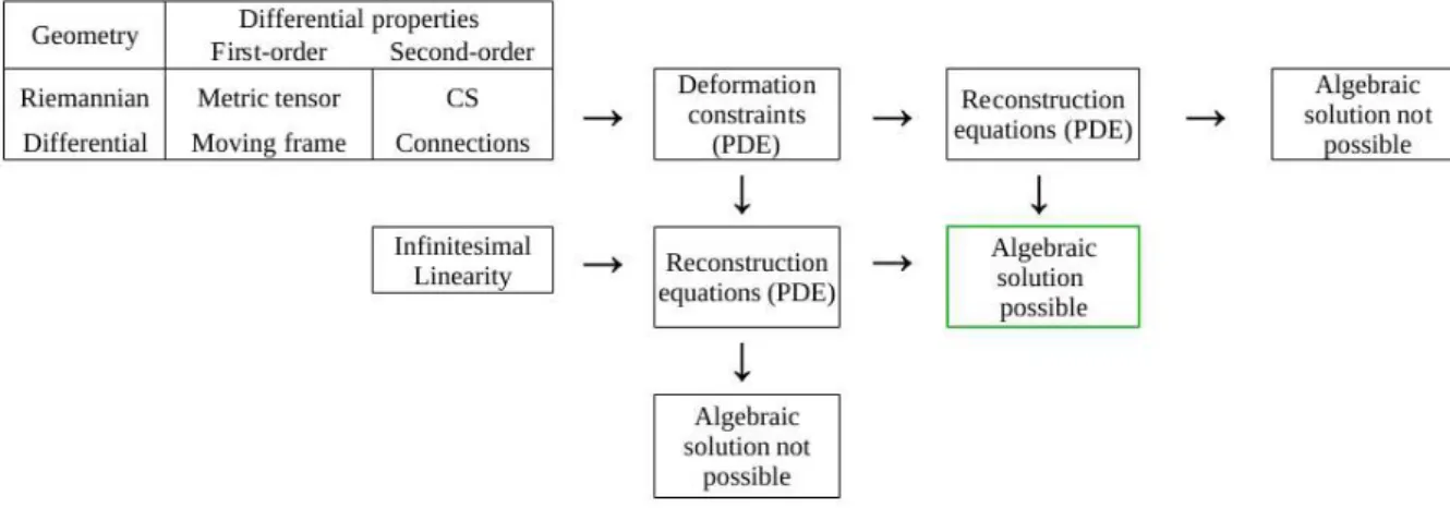
This theoretical framework leads to local solutions to deformable 3D reconstruction in terms of PDE which we solve algebraically (see figure 1.4 for more details). This frame-work represents surfaces analytically. Therefore, it is very easy to change surface definition which makes it very easy for this framework to adapt for different representations. By
ex-Figure 1.4: A broad overview of the problem. Moving frames and connections are the generalisa-tion of the concepts of metric tensors andCS from Riemannian geometry. We use them to express differential constraints in terms ofPDE. The manipulation of these constraints with or without the
ILassumption leads to reconstruction equations that are also PDE. ILis not necessary to find these equations, however we use it to simplify the problem. These reconstruction equations may or may not have an algebraic solution. Here, an algebraic solution implies that the equations can be solved locally at each point. In this thesis, we solve the equations with possible algebraic (or local) solution.
pressing the deformation constraints in terms of the moving frame and using our theorem of transfer of connections, we present solutions to deformable 3D reconstruction for various deformations like isometry, conformity, skewless or equiareal. The solution toNRSfM under a) isometric/conformal deformations is given by solving a system of two cubics, b) skewless
deformations is given by solving a system of two septics (exploiting the first and second-order derivatives of the warps) in terms of two variables only.
We show that Iso-NRSfM (our first contribution) can be obtained using this framework as well. In this solution, we chose isometry to be solved as conformity as it makes the problem simpler to solve.
Our framework is directly extended to SfT. The existing solutions to isometric and conformalSfT [Bartoli et al.,2015] can be derived using this framework. We obtain anSfT solution to a) isometric/conformal and equiareal deformation as two linear expressions, b) skewless deformation as a system of two cubics in terms of two variables. These expressions exploit the first and the second-order derivatives of the warps.
Due to our theorem of transfer of connections across smooth surfaces using the inter-image warps, we propose a solution to SfT which is independent of the deformation constraints and only imposes deformation to be locally smooth. SfT has previously been solved under the assumption of smooth deformation in [Bartoli and ¨Ozg¨ur, 2016]. We compare it with our results of SfT. [Salzmann et al., 2007] discussed that such a solution is not well-posed, however, we show that our solution to smooth deformations is well-posed. We discuss the reasons which make it well-posed.
Summing up, the proposed framework has the following features. 1) It is a unified mod-elling framework for NRSfM (and SfT) using differential geometry assuming IL, which can be extended to various deformations. 2) It brings the solutions to isometric/conformal and skewless NRSfM as a set of two cubic and septic polynomials respectively in terms of two variables for any number of views. 3) It brings the solutions to isometric/conformal and equiareal SfT using a linear system of two equations in two variables only. 4) It brings the solution to skewlessSfT by solving a cubic system of two equations in two variables only. 5) It also brings a solution to SfTfor smooth deformations which is also a system of two linear equations in two variables only.
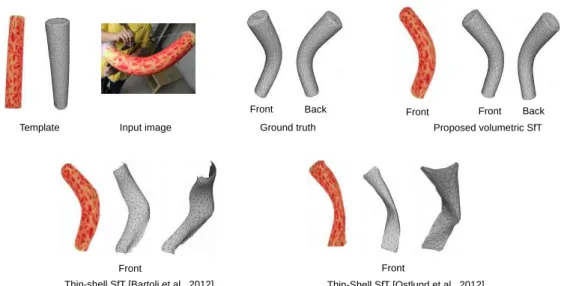
Contribution 3: Shape-from-Template for volumetric objects. As discussed earlier, existingSfTmethods are thin-shellSfTessentially, as they are designed for thin objects such as a piece of paper. However, while thin-shellSfThandles thicker objects such as the woggle of figure 1.5 or a foam ball, it does not fully exploit the strong constraints induced by the object’s non-empty interior.
We bringSfTone step further by introducing volumetric SfT, defined as anSfTmethod which uses a deformation constraint on the object’s outer surface and interior. An example is shown in figure 1.5. Volumetric SfT reconstructs the object’s interior deformation, which is not reconstructed by thin-shellSfT, and reconstructs the object’s outer surface more accu-rately than thin-shell SfTthanks to the stronger deformation constraint it uses. Volumetric SfT is challenging as only the front part of the object’s surface is visible in the image: the object’s back surface and interior have to be inferred with no direct visual observations.
It is important to note that strictly speaking, isometry leads to rigidity in volumes. Only rigid volumetric objects can preserve geodesic-distances while undergoing deformation. We
1.3. CONTRIBUTIONS 11
Proposed volumetric SfT
Template Input image Ground truth
Front Front Back
Front Back
Thin-shell SfT [Bartoli et al., 2012] Thin-Shell SfT [Ostlund et al., 2012]
Front Front
Figure 1.5: Volumetric SfTversus thin-shell SfT. Existing methods are thin-shell SfT. They use deformation constraints on the object’s surface. For instance, [Bartoli et al., 2012] uses isometric constraints on the object’s visible (front) surface and reconstructs the object partially, while [Ostlund¨ et al., 2012] uses isometric constraints on the object’s whole closed outer surface and reconstructs it entirely. Volumetric SfTuses deformation constraints on the object’s surface and interior. This greatly improves reconstruction accuracy and facilitates reconstruction of the object’s interior. In this example, the thin-shell SfTmethods [Bartoli et al., 2012; Ostlund et al.¨ , 2012] reach a 3D error of 20 mm and 13 mm respectively on the visible surface, while the proposed volumetric SfT method reaches a 3D error of 7 mm. It reconstructs the non-visible (back) surface, for which no visual data is available, with a 3D error of 17 mm.
propose to instantiate volumetric SfT using the As-Rigid-As-Possible (ARAP) deformation model (a relaxation of isometry), which has been used extremely successfully in Computer Graphics [Sorkine and Alexa.,2007;Zhang et al.,2010]. TheARAPmodel maximises local rigidity while penalising stretching, sheering and compression. More specifically, ARAPhas been widely used to perform mesh editing of animated characters [Zhou et al.,2005;Zollh¨ofer et al.,2012] because the resulting deformations locally preserve the object’s structure.
Contrary to thin-shell SfT, volumetric SfT is largely unexplored. Recently, [Innmann et al., 2016] proposed a method that reconstructs the closed thin-shell surface of the de-formable object in real-time. This method is named “VolumeDeform” however it does not reconstruct the interior of the object. The closest method to volumetricSfT is perhaps [ Vi-cente and Agapito.,2013], whereSfThas been combined with silhouette-based reconstruction. However this method requires stronger image cues, including silhouette and point correspon-dences, and recovers two-way ambiguous shape solutions. In contrast, we solve volumetric SfTwithout restricting the topology of the object and using the perspective camera. By using ARAP, our method preserves the object’s interior structure while jointly reconstructing the deformation of the object’s full outer surface and interior, as illustrated in figure1.6. ARAP volumetric SfT involves solving a non-convex constrained variational optimisation problem. We discretise the object’s volume and relax the constraints to convert the variational problem into an unconstrained non-linear least-squares optimisation problem. This problem can then be solved with standard numerical solvers such as Levenberg-Marquardt. We propose two
3D template with a
virtual cylinder inside Reconstructed deformation of the cylinder for two deformations of the object
Figure 1.6: As opposed to thin-shellSfT, volumetricSfTreconstructs the object’s interior deforma-tion. In this example using the data from figure 1.5, a virtual cylinder is placed inside the woggle’s template. It is then deformed using the deformation reconstructed by volumetric SfTto aid visual-ization of the object’s reconstructed interior deformation. The second deformation is the one shown in figure1.5.
initialisation methods. These methods use isometric thin-shellSfT and propagate the result through the object’s volume.
The proposed contribution has the following features. 1) We show that isometry in volumes is essentially a local rigidity or inextensibility constraint. 2) We solve volumetric SfTin two steps: initialisation and refinement. 3) We propose two methods for initialisation. 4) We perform refinement in two ways: minimising L1 and L2 norms. 5) Experimental results on synthetic and real data show that volumetric SfT improves accuracy to a large extent compared to state-of-the-art thin-shell SfTmethods.
Thesis layout. We have divided this thesis into 7 chapters. We discuss the state of the art in chapter 2, mathematical preliminaries in chapter 3. Chapters 4, 5 and 6 give our first, second and third contributions. Chapter 7 presents our conclusions and perspectives for future work.
Chapter
2
Related Work
In this chapter we discuss the existing works onSfTandNRSfMthat use motion as a visible cue in two sections. We sub-categorise these methods based on the constraints they use. Most of these methods are designed for thin-shell objects but we also discuss the works that are related to volumetric objects.
2.1
Shape-from-Template
The SfT methods were introduced much later than NRSfM but they evolved quickly. Now there are stable and real-time SfT methods [Collins and Bartoli, 2015; Ngo et al., 2016]. In general, SfT uses a 3D template of a thin-shell object. This is a very strong prior and makesSfT a better-posed problem thanNRSfM. We classify current SfTmethods into two categories: initialisation and refinement methods. The initialisation methods are the ones which achieve a fast solution to SfT using deformation constraints. They do not employ a heavy non-convex optimisation to minimise a cost which consists of a set of constraints such as deformation, smoothness or reprojection which is the case with refinement methods. Refinement methods are computationally expensive but more accurate. However, they need to be initialised. The performance of these methods depends on the accuracy of initialisation. A good initialisation can significantly reduce their computation time. We recall that the currentSfT solutions are for thin-shell objects only,SfTfor volumetric objects has not been proposed however, we discuss some of the works that use non thin-shell models.
Most of the SfT methods exploit physics-based modelling. Most of them use isometry as a physical prior but there are some solutions that use elasticity [Haouchine et al., 2014; Malti et al.,2013], the particle model [Ozg¨¨ ur and Bartoli,2016] or smoothness [Bartoli and
¨
Ozg¨ur,2016]. We organise these two categories of initialisation and refinement into methods that employ isometric and non-isometric constraints. We now discuss these two categories of methods.
2.1.1 Thin-Shell Initialisation Methods
2.1.1.1 Isometric Constraints
Most of the initialisation methods use isometry as a deformation prior. Isometry is a physi-cal prior on deformation which can be seen as lophysi-cal rigidity. Isometry preserves the geodesic distances between points on a surface undergoing deformations. Therefore stretching or shrinking of the surfaces is not allowed. Inextensibility is a relaxation of isometry. It means that the Euclidean distances between the neighbouring points on the deformed surfaces are always lower than or equal to the corresponding geodesic distances on the original surface. Figure 5.1 shows two surfaces S1 and S2 related by a deformation. The isometric and
inex-deformation
Figure 2.1: A surface S1 transforms to surface S2 due to a deformation. The points (P1, P2) on S1
transform to (Q1, Q2) on S2.
tensibility constraints on the points (P1, P2) on S1 and (Q1, Q2) on S2 in terms of distances
between the points can be written as
kQ2− Q1kg = kP2− P1kg isometry constraint
kQ2− Q1k2 ≤ kP2− P1kg inextensibility constraint
(2.1)
where k.k2 represents the Euclidean distance and k.kg represents the geodesic distance
be-tween two points on a surface. Therefore, we can see that intextensibility is a relaxed form of isometry. However, expressing geodesics on an arbitrary surface is not easy. Therefore, most of the methods approximate the geodesics with euclidean distances by assuming that the points are very close to each other. For example, the geodesic of (Q1, Q2) on S2 can be
written as the Euclidean distance between them given that Q2 is close enough to Q1. The
sense of closeness or neighbourhood of these points are defined by the methods. Inextensibil-ity needs to be combined with maximum depth in order to prevent the reconstructed surface from shrinking. This is called as Maximum Depth Heuristics (MDH).
We now discuss the initialisation methods that use inextensibilty and isometry constraints in two sections.
2.1.1.2 Inextensibility Constraints
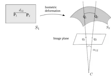
[Perriollat et al., 2011] was the first method to model isometry using the inextensibility constraint (2.1). It is based on the MDH. It finds a solution to SfT by maximising depth heuristically while imposing inextensibility constraints. Figure2.2shows two surfaces related with an isometric mapping. Consider Q1 at a distance µ1 from the camera. Assuming that
2.1. SHAPE-FROM-TEMPLATE 15
Isometric deformation
Image plane
Figure 2.2: A surface S1 transforms to surface S2 due to an isometric deformation. The points
(P1, P2) on S1transform to (Q1, Q2) on S2. The sightlines of the two points (Q1, Q2) from the camera
C pass through (q1, q2) on the image plane.
sightlines from the camera C. Therefore, we can write
Q1= µ1 0 0 , Q2= µ2cos (α12) µ2sin (α12) 0 . (2.2)
Using this parametrisation of the points, the inextensibility constraint in equation (2.1) gives the upper bound of µ1 as
µ1 ≤
d12
sin α12
, (2.3)
where d12 is the geodesic distance between the 3D points P1 and P2 in the template. This is
the upper bound on the depth of each point. It is chosen to be the minimum upper bound of all the neighbouring points such that the inextensibility constraint (2.1) is satisfied.
[Salzmann and Fua,2011] made an improvement by modelling this problem as an Second-order Cone Program (SOCP) which can be globally solved using convex optimization. The method parametrises 3D points as the back-projection of 2D image points. Therefore any point Qi can be expressed as
Qi = zi " qi 1 # , (2.4)
where zi is the depth at the ith point and qi is the normalized image point. The idea is to
maximise the sum of all the depths zi such that the inextensibility constraint (2.1) is satisfied.
This method uses a learned space of deformations using linear local models for small patches. This limits the applicability of this method to surfaces whose linear local models are known. However, it shows good performance when there is enough perspective in the images. [Brunet et al., 2014] proposed an initialization method based on inextensibility constraints solved using MDH. It used a parametric representation of surfaces using cubic B-splines [Dierckx,
1993] which reduces the dimensionality of the problem and provides a solution faster. [Ngo et al., 2016] proposed a modified approach, where the method uses a laplacian smoothness prior along with inextensibility constraints. The laplacian of the template is calculated which is assumed to be preserved under the deformation. The laplacian is linearly parametrised and therefore, the problem can be solved usingLLS. It is used as an initialisation method to the real-time solution to SfTproposed in [Ngo et al.,2015].
The above-mentioned methods use inextensibility constraints which is a relaxation on isometry and therefore, it is not a strict physical constraint. A more accurate representation of deformation constraints is possible by using differential modelling which we discuss next.
2.1.1.3 First-Order Differential Isometric Constraints
Recently, [Bartoli et al., 2015] proposed a local analytical solution to SfT using a warp and first-order differential isometric constraints. It shows that SfT is a well-posed problem for isometric deformations. It expresses the constraints in terms of first-order PDEand finds an algebraic solution to it. Since the method is analytical, it is very fast. However, it suffers with instabilities under near-affine conditions. [Chhatkuli et al.,2016b] proposed an improvement on these solutions to find an analytical stable solution to depth using the gradient of the depths which were otherwise discarded in [Bartoli et al.,2015].
The success of these SfT methods inspires us to extend the physics-based differential modelling of deformation to NRSfM as well. We use differential geometry to formulate the
NRSfM and SfTproblems in terms of PDEand we find algebraic solution to them.
2.1.1.4 Non-Isometric Constraints
[Bartoli and ¨Ozg¨ur,2016] proposed to solveSfTby using only smoothness as a deformation prior. The solution is unique and obtained by solving anLLSproblem. It finds the solution to SfT using reprojection constraints and a smoothness constraint for a fixed scale. The problem with this method is that smoothness is a very weak constraint which can make this method unstable.
[Bartoli et al.,2015] also proposed an analytical solution to conformalSfT. This solution was also formulated using PDE and solved algebraically. Even though this method suffers form instabilities, it usually performs better or as well as isometricSfT[Bartoli et al.,2015]. Therefore, differential modelling proves to be a good tool for non-isometric deformations as well.
2.1.2 Thin-Shell Refinement Methods
These methods formulate global deformation constraints and solve them by using a non-convex optimisation. Therefore, these methods need to be initialised. The initialisation methods discussed in the previous section can be used to initialise these methods. In fact, initialisation methods should always be combined with refinement methods in order to get the best possible reconstruction. The accuracy of initialisation methods makes the refinement
2.1. SHAPE-FROM-TEMPLATE 17
significantly faster. [Chhatkuli et al.,2016b] showed results by initialising [Brunet et al.,2014] with their result. They achieved an almost real-time reconstruction. [Collins and Bartoli, 2015] made an improvement on this and achieved a real-time reconstruction. We now discuss the refinement methods that use isometric and non-isometric constraints in the next two sections.
2.1.2.1 Isometric Constraints
[Brunet et al., 2014] proposed the first solution to SfT which optimises a statistically opti-mal cost. The cost is composed of three errors: 3D back-projection, differential isometric constraints and smoothness. The 3D back-projection error (Ereprojection) accounts for the
difference when the 3D points of the deformed shape project back to the corresponding in-put image points. The differential isometric constraint error (Eisometry) forces that isometry
holds at infinitesimal level. It ensures that the deformed shape is isometric. The smoothness error (Esmooth) forces the solution to be smooth. This problem is non-convex and relies on
iterative local optimization such as Levenberg-Marquardt which requires to be initialised and has a high computation time. The cost is written as
Cost = Ereprojection+ lisometryEisometry+ lsmoothEsmooth, (2.5)
where the two parameters lisometry and lsmooth are weights to the isometric and smoothness
constraints and need to be tuned. We use a similar cost in order to find a solution to volumetric SfT.
[Yu et al., 2015] introduced a temporal smoothness constraint in addition to the above mentioned constraints in order to improve the refinement.
2.1.2.2 Non-Isometric Constraints
[Malti et al.,2011;Ngo et al.,2015] model deformation as conformal and use the pixel intensity error instead of the reprojection error. [Ngo et al.,2015] is initialised with [Ngo et al.,2016] and handles occlusions and poorly textured surfaces.
[Ozg¨¨ ur and Bartoli,2016] proposed a solution toSfTby expressing the object as a set of particles where deformation acts as a set of forces on it. It uses deformation and reprojection constraints and finds a solution by evolving particles to achieve a global equilibrium due to the action of various forces (including gravity). It uses boundary points to fix the solution.
[Haouchine et al., 2014; Malti et al., 2013] proposed a solution to SfT for extensible surfaces by modelling deformation with elasticity. The idea is to minimise the stretching energy such that the reprojection constraint and boundary points are satisfied.
SfTmethods using non-isometric constraints are mostly solved using non-convex optimi-sation.
2.1.3 Shape-from-Template for Volumetric Objects
Volumetric objects have non-zero thickness. SfTmethods using elasticity [Haouchine et al., 2014;Malti et al.,2013] require the surface model to include thickness, which must however be ‘small’ so that extension along normal direction may be neglected. In continuum mechanics, this means that the thickness is at least ten times smaller than the object’s largest dimension. Therefore, these methods are categorised as thin-shell methods. They require one to provide the Young modulus of the object’s material and, more importantly, boundary conditions expressed as a set of known 3D point coordinates, which may restrict their applicability.
A related goal was pursued in [Vicente and Agapito., 2013] where a silhouette-based method was combined with SfT. The template is also reconstructed from a reference image using a silhouette-based method inspired from [Oswald et al., 2012]. This method recon-structs objects that have a plane of symmetry parallel to the image plane and does not infer concavities, which is also a limitation of most silhouette-based methods [Oswald et al.,2012; Prasad et al., 2006]. The template is then deformed using a data term based on silhouette, area and orthographic reprojection constraints. The deformation model extends thin-shell isometry by placing virtual nodes in the object’s interior, with the objective of preserving the object’s volume.
2.1.4 Relationship to our Work
In chapter 4, we propose a modelling framework for SfT using differential geometry. This framework is coherent with methods based on differential modelling [Bartoli et al.,2015] and is general, therefore, other deformation models can be used. We also propose a solution to SfTassuming that the deformation is smooth. This means thatSfTcan be solved analytically for any kind of deformation without explicitly modelling the deformations.
In chapter5, we propose volumetricSfTwhich, in contrast to thin-shellSfT, recovers the deformation of the object’s outer surface and interior. It formulates the deformation globally in terms of a cost function and minimises it using non-convex optimisation.
2.2. NON-RIGID STRUCTURE-FROM-MOTION 19
2.2
Non-Rigid Structure-from-Motion
The first solution toNRSfMfor thin-shell objects was proposed in [Bregler et al.,2000] which modelled deformation using a low-rank shape-basis. It assumes that the shape of an object can be represented as a linear combination of a low-dimensional shape-basis. We discuss the two categories of NRSfM methods based on the modelling framework: statistics-based modelling and physics-based modelling.
2.2.1 Methods with Statistics-based Models
Starting from the work of [Bregler et al.,2000], the low-rank shape-basis has been the most commonly used shape prior in NRSfM. It is a statistical prior on a set of 3D point cor-respondences expressed in terms of point corcor-respondences in images that forces the matrix containing these correspondences to have a fixed low-rank. This matrix can be further de-composed into a shape-basis and their weights. Inspired from this method, [Akhter et al., 2009] proposed NRSfM which modelled deformation as a set of trajectory basis. We discuss statistics-based methods under these two categories.
2.2.1.1 Low-Rank Shape-Basis
For N images, the image observation matrix consisting of the P matched point correspon-dences across the images is written as
W = u11 . . . u1P v11 . . . vP1 .. . . .. ... uN1 . . . uNP vN1 . . . vPN , (2.6)
where (uji, vij) represents the image coordinates of the ith point on the jth image. Any shape can be written as a linear combinations of the K shape-basis Bi. Therefore the shape Si of
the ith image can be written as
Si=
K
X
t=1
litBt, (2.7)
where each shape-basis Bt is 3 × P matrix and lti is the set of weights that decide the scale.
Projecting these shape-basis on images under a scaled orthographic projection, we can write the observation matrix as
W = u11 . . . u1P v11 . . . vP1 .. . . .. ... uN1 . . . uNP v1N . . . vNP = l11R1 . . . l1KR1 .. . . .. ... l1NRN . . . lKNRN B1 .. . Bk = QB, (2.8)
where Ri consists of the first two rows of the camera projection matrix. The goal is to decompose W into two matrices Q and B which contain the information of the scale and the set of shape-basis respectively. Once Q and B are found any shape can be written using equation (2.7). Q can be further decomposed in order to find the pose.
[Bregler et al.,2000] used Singular Value Decomposition (SVD) to decompose W into Q and B by fixing K as a low positive integer. Q and B are called the coefficient matrix and shape-basis matrix respectively. This problem is non-convex and suffers from ambiguities in the solution to the shape-basis. [Del Bue et al., 2004] proposed a non-linear refinement to improve the solution. However in order to deal with these ambiguities, different kinds of priors were proposed by various methods:
1) [Del Bue, 2008] proposed to use shape-basis priors to constrain the B matrix. The idea is to estimate the shape-basis for some known 3D shapes and use them along with the unknown shape basis in order to estimate the shapes for all the images. This means that some of the basis in B are already calculated using few known 3D shapes and W is decomposed in a way that these known shape bases do not change. Given that the first b elements of B are known, the shape prior L according to [Del Bue,2008] is given by
L = N B1 .. . Bb = N B. (2.9)
The joint decomposition of W and L into Q, N and B improves the conditioning of the shape. [Tao and Matuszewski, 2013] extended this idea to allow shapes to have non-linear deformations by allowing L to be non-linear. B is found from a manifold whose embeddings are learnt from a representative training dataset of the deformable object under consideration. This is not a traditionalNRSfM method (as it heavily relies on training to find B), however it does highlight the success of manifold learning.
2) [Torresani et al., 2001] solves this problem by adding a shape regulariser term that imposed spatial smoothness in the observed shape using an iterative optimisation.
3) [Olsen and Bartoli,2008] solves this problem by optimising the shape-basis using spatial and temporal smoothness priors.
4) [Bartoli et al.,2008] uses deformation modes and closeness of points in the mean shape as priors. It solves the ambiguity by using a low-rank coarse-to-fine shape model which prioritises the deformation modes that give the coarsest deformations.
5) [Fayad et al.,2010] proposed to model the deformations (patch-wise) with quadratic models where the linear modes allow shearing and stretching, quadratic modes allow bending and the mixed modes allow the twisting of the surfaces. These modes are optimised for each (overlapping) patch using the temporal smoothness priors. Then they are stitched together to obtain a global surface.
5) [Akhter et al.,2009] shows that an ambiguity in the SVDdoes not necessarily lead to an ambiguous reconstruction. They introduced a correction matrix that can be used to obtain
2.2. NON-RIGID STRUCTURE-FROM-MOTION 21
a unique solution. They showed that the camera orthonormality conditions are sufficient to find the correction matrix. [Dai et al., 2012] proposed a more efficient solution to find this matrix by minimising the trace of the shape-basis. Trace-minimisation is a tighter constraint than rank-minimisation (used in [Akhter et al.,2009]). [Garg et al., 2013a] also used trace minimisation of the correction matrix in order to find the low-rank shapes. They formulated the problem as a global variational energy minimisation problem. The goal is to minimise the trace of the shape-basis, reprojection error and the total spatial variation. This method performs dense reconstruction and yields good results for faces. However, this algorithm is computationally very expensive.
Most of these methods express shapes as a linear combinations of shape-basis. This forces the deformations to be linear. Therefore these methods are applicable to simple deformations such as a talking face. They do not cope up with the larger deformations such as a walking man or a tree moving due to the wind unless more constraints are provided.
2.2.1.2 Low-Rank Trajectory-Basis
[Akhter et al.,2009] proposed to replace the shape-basis by a trajectory-basis in the formu-lation suggested by [Bregler et al., 2000]. This method can easily reconstruct larger defor-mations than the above-mentioned methods. The fundamental idea behind this method is to express the trajectory of a point on an image as a linear combination of the trajectory-basis. The trajectory-basis are obtained using a Discrete Cosine Transformation (DCT) basis. [Akhter et al.,2009] proposed to decompose the image observation matrix W in equa-tion (2.6) into R and T using SVD, where R contains the Ri (the first two rows of camera projection matrix for the ith image) and T is the trajectory-basis matrix.
[Gotardo and Martinez,2011] proposed a solution that uses additional higher frequencies of the DCT basis in order to estimate large deformations better than [Akhter et al., 2009]. This method first estimates the 3D using trajectory-basis. It then estimates the shape-basis by applying a kernel transformation which generalises the inner product with a radial basis function.
[Torresani et al., 2008] also uses a parametric representation of shape and trajectory-basis and finds 3D by estimating these parameters using Probabilistic Principal Component Analysis.
These methods can handle large deformations better than the low-rank shape model methods but they still need video-sequences or short-baseline data to achieve good results.
Table2.1summarises the statistics-basedNRSfMmethods. All these methods use the or-thographic projection model. All these methods solveNRSfMwith a non-convex formulation except [Dai et al.,2012] which uses a convex relaxation.
Most of the statistics-based methods use orthographic camera projection which may lead to flip ambiguities in the reconstruction. Also, these methods are designed for short-baseline images and therefore, they cannot handle large deformations. For good results, these methods need a large number of views.
Method Type of basis Additional priors Complexity of basis
[Bregler et al.,2000] Shape - Linear
[Del Bue,2008] Shape Shape Linear
[Tao and Matuszewski,2013] Shape Shape Non-linear
[Dai et al.,2012] Shape - Linear
[Torresani et al.,2001] Shape Spatial smoothness Linear [Olsen and Bartoli,2008] Shape Spatio-temporal smoothness Linear [Bartoli et al.,2008] Shape Deformation modes, point closeness Linear
[Akhter et al.,2009] Trajectory - Linear
[Torresani et al.,2008] Shape, trajectory Spatio-temporal smoothness Linear [Gotardo and Martinez,2011] Shape, trajectory - Non-Linear
Table 2.1: Summary of statistics-basedNRSfMmethods
2.2.2 Methods with Physics-based Models
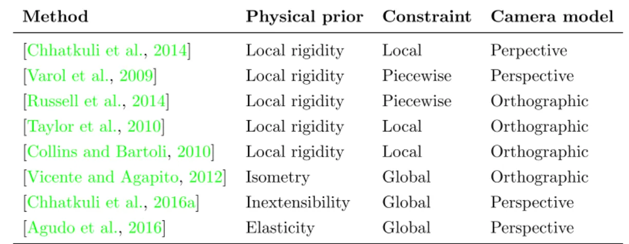
For a long time, the focus of the research community has been on the statistics-based mod-elling of deformation. Physics-based modmod-elling forNRSfM is rather recent. In general, these methods use the physical properties of thin-shell objects to model deformation as in SfT. They can handle more complex deformations and work with fewer images than methods with statistics-based modelling. Most of these methods, for example [Chhatkuli et al.,2014,2016a; Collins and Bartoli,2010;Russell et al.,2014;Taylor et al.,2010;Varol et al.,2009;Vicente and Agapito,2012] use isometry as a deformation model except [Agudo et al., 2016] which models deformations using elasticity. [Agudo et al.,2016] first reconstructs the surface by as-suming that there are no deformation acting on it (basicallySfM) and then uses this solution the predict the deforming shapes. Therefore, this method resembles SfT even though it is presented as aNRSfM method by the authors.
[Collins and Bartoli,2010;Taylor et al.,2010] approximate isometry with a rigid rotation and translation at a local (or piecewise) level. For example, [Collins and Bartoli,2010; Tay-lor et al.,2010] solved NRSfM by expressing isometry as local rigidity with an orthographic camera projection. [Taylor et al., 2010] finds sets of 3 rigid points reconstructed using SfM whereas [Collins and Bartoli,2010] performs automatic clustering of point sets. These meth-ods rely on finding the 3 points in a close neighbourhood in order to make sure that the assumption of rigid transformation holds. Another approximation was made by [Russell et al.,2014; Varol et al., 2009], they exploited isometry as piecewise-rigidity. [Russell et al., 2014] computes fundamental matrices [Hartley and Zisserman,2000] to obtain the solution to surface normals. However, fundamental matrices may be unstable in case of small patches. An improvement on [Varol et al.,2009] was proposed by [Chhatkuli et al., 2014] which defines isometric constraints between points that are infinitesimally close to each other while [Varol et al., 2009] defines these constraints on a small patch (assuming piecewise-rigidity). Both of them assume perspective projection. [Chhatkuli et al., 2014] assumes the surface to be a set of infinitesimal planes while [Varol et al.,2009] assumes the surfaces to be represented as a set of planar patches. They then obtain a homography between the corre-sponding normalised image points of the planes and use homography decomposition [Malis and Vargas, 2007] to obtain the surface normals. The surface normals thus obtained have
![Figure 1.1: 3D reconstruction methods. For rigid objects, SfM is a widely used method (Images taken from [Snavely et al., 2007])](https://thumb-eu.123doks.com/thumbv2/123doknet/14596121.543260/23.892.111.782.449.916/figure-reconstruction-methods-objects-widely-method-images-snavely.webp)
![Figure 1.3: Comparison of Iso-NRSfM (with and without IP) with [Chhatkuli et al., 2016a].](https://thumb-eu.123doks.com/thumbv2/123doknet/14596121.543260/28.892.135.792.768.1013/figure-comparison-iso-nrsfm-ip-chhatkuli-et-al.webp)