Data Aggregation for Data Analytics in Medical Device Supply Chains

(1)

Data Aggregation for Data Analytics in Medical Device Supply Chains

by

Gabriela Lamas Oporto B.S. in Biomedical Engineering

and Sherif Alhalafawy B.S. in Electrical Engineering

SUBMITTED TO THE PROGRAM IN SUPPLY CHAIN MANAGEMENT IN PARTIAL FULFILLMENT OF THE REQUIREMENTS FOR THE DEGREE OF

MASTER OF APPLIED SCIENCE OR MASTER OF ENGINEERING IN SUPPLY CHAIN MANAGEMENT AT THE

MASSACHUSETTS INSTITUTE OF TECHNOLOGY May 2020

The authors hereby grant to MIT permission to reproduce and to distribute publicly paper and electronic copies of this capstone document in whole or in part in any medium now known or hereafter created. Signature of Author: ____________________________________________________________________

Department of Supply Chain Management May 8, 2020 Signature of Author: ____________________________________________________________________ Department of Supply Chain Management

May 8, 2020 Certified by: __________________________________________________________________________ James B. Rice, Jr. Deputy Director for Center for Transportation and Logistics Capstone Advisor Certified by: __________________________________________________________________________ Dr. Tugba Efendigil Research Scientist for Center for Transportation and Logistics Capstone Co-Advisor Accepted by: __________________________________________________________________________ Professor Yossi Sheffi Director, Center for Transportation and Logistics Elisha Gray II Professor of Engineering Systems Professor, Civil and Environmental Engineering

(2)

Page 2 of 37

Data Aggregation for Data Analytics in Medical Device Supply Chains by

Gabriela Lamas Oporto and

Sherif Alhalafawy

Submitted to the Program in Supply Chain Management on May 8, 2020 in Partial Fulfillment of the

Requirements for the Degree of Master of Applied Science or Master of Engineering in Supply Chain Management

ABSTRACT

Product visibility in the medical device supply chain is a challenge for suppliers, distributors, and hospitals. The lack of visibility makes managing inventory complex, and it is made more difficult when businesses have a segregated distribution model. In this model, a surplus of systems collects inventory data at the supply chain nodes, but the data is not integrated due to system barriers. This aspect of ‘big data’ is a current problem multiple supply chains are facing as they look towards future data analytic capabilities. In this capstone, we evaluated the potential of integrating the sponsoring company’s data sets from fragmented planning systems in enabling advanced data analytics and visualization that can improve inventory management. We successfully created a data aggregation tool after cleaning and transforming the data sets and performed data analysis on the aggregated data. SKU segmentation was completed, and their inventory distribution analyzed. Results support using aggregated data sets for data analytics in medical device supply chains. We recommend that the sponsoring company integrate the tool into their business processes and use customer centric data to enhance their inventory management. The medical device industry struggles with product visibility and the lack of connectivity is a barrier, but as companies continue to strive towards aggregated systems for data analytics, these capabilities would lay the framework for better inventory management in their distribution networks. Capstone Advisor: James B. Rice, Jr.

Title: Deputy Director for Center for Transportation and Logistics Capstone Co-Advisor: Dr. Tugba Efendigil

(3)

Page 3 of 37 ACKNOWLEDGMENTS

We would like to thank our capstone advisors and mentors, James B. Rice, Jr. and Dr. Tugba Efendigil, for their guidance and support while writing this capstone project. We would also like to thank those we have worked with from our capstone partner company, for sharing information, retrieving data when necessary for our analyses, and devoting their time to communicate with us. In addition, we want to express an immense appreciation to our colleagues who helped us program the code required to create the big data aggregation tool, making this capstone a success: Kristian From, Brett Elgersma, Saikat Banerjee, and Zhehao Yu. Pamela Siska was incredibly helpful in structuring our research and editing our writing. Finally, we would like to thank our parents and family for their support and encouragement throughout the completion of our master’s program. Thank you.

(4)

Page 4 of 37

List of Figures

Figure 1: The Company’s Distribution Network ... 7

Figure 2: Information Shared and Decisions made in TSC (Kamalapur et al. (2013)) ... 15

Figure 3: Information Shared and Decisions made in VMI (Kamalapur et al. (2013)) ... 16

Figure 4: Information Shared and Decisions made in CPFR (Kamalapur et al. (2013)) ... 16

Figure 5: Big Data Approach Summary ... 20

Figure 6: Original Internal DC and Field Inventory Data File Format ... 21

Figure 7: New Internal DC and Field Inventory Data Frame Format ... 21

Figure 8: Original Forecast Accuracy Data File Format ... 22

Figure 9: New Forecast Accuracy Data File Format ... 22

Figure 10: Original Sales Data File Format ... 22

Figure 11: New Sales Data File Format ... 22

Figure 14: Sample of Aggregated Data ... 24

Figure 15: Sales “Ship-to” Volume per State ... 29

Figure 16: Inventory volume per state ... 30

Figure 17: Sales and Inventory Volume Comparison by State ... 30

List of Tables

Table 1: Data Sets Provided for the Company's Product Platform ... 19

Table 2: Attribute Summary Details ... 19

Table 3: Key Data Source Summary ... 20

Table 4: Data Segmentation Summary ... 27

Table 5: Data Aggregation Summary Part 1 ... 28

(6)

Page 6 of 37

Chapter 1: Introduction

The medical device industry is valued at more than $140 billion in the U.S., representing approximately 45% of the global market, with an annual growth rate of 4.6% (Medidata, 2018). As the market continues to grow, customers of medical device companies are facing challenges such as increasing inventory costs and forecasting difficulty (Medidata, 2018). In response to these challenges, customers are looking for suppliers who offer not only a physical product but an entire solution (Byrnes and Wass 2020). To stay competitive, medical device companies recognize the need to create a customer value solution that increases customer service and decreases costs for the overall system. Specifically, the industry is looking for a solution that addresses the increasing costs associated with inventory in the field (e.g. 3rd_{party distributors, hospitals, or private clinic facilities), costs that are} impacting the bottom line of suppliers and their customers. The problem is that there is limited inventory visibility between customers, distributors, and suppliers to enable efficient troubleshooting. Medical device companies are working to integrate data sources to enable product visibility and create an agile, end-to-end solution that improves healthcare supply chain costs and give people around the world access to safer and more affordable devices (Attainia, 2018).

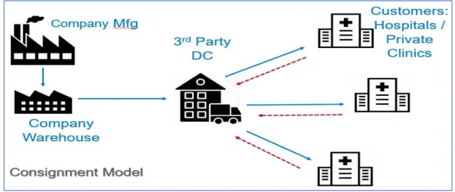
The medical device company sponsoring this capstone is addressing a unique set of challenges due to the lack of product visibility throughout their supply chain, which comprises manufacturing, warehouses, distributors, and customers. In this capstone, we focus on one of the company’s franchises that uses a consignment inventory model. Their customers are hospitals and private clinics. In the rest of this paper, we will refer to the franchise as ‘the Company.’

Unlike many medical device companies that use a traditional inventory model, the Company’s franchise follows a consignment business model, which means their inventory is owned by the Company until the device is used by a medical professional. This means that when the Company assigns its inventory to 3rd party distributors, the Company still owns the inventory, but they can no longer track its location, making it a challenge to forecast sales. This can result in approximately 400 days of supply on hand for many of the company’s SKUs. Their inventory is either held at a 3rd_{party distributor or in the} field (e.g. hospitals or private clinic facilities). See Figure 1 for a diagram of the Company’s distribution channel.

(7)

Page 7 of 37

Figure 1: The Company’s Distribution Network

The Company’s problem is aligned with that of the industry; the Company is holding too much inventory and they are struggling to isolate the root cause and the right opportunities to reduce this inventory. We believe the lack of data source integration and lack of product visibility in their downstream operations are the barriers. The Company has data for inventory, sales, and forecast accuracy but the sources are segregated, and they have not been able to combine them due to current system limitations. We outlined two research questions:

1. How can we integrate inventory, sales, and customer service data to improve data analytics capabilities to drive finding business insights?

2. How can we use data integration to identify SKUs to reduce costs associated with excess inventory in the field?

Our hypothesis was that the excess inventory in the field may be primarily driven by the lack of integrated inventory systems; the inherent habit of overstocking in the field to avoid stock outs; and delayed transactions at the point of use (this delay occurs because once a device is used, the purchase order is done manually and not electronically which means there is a lag as orders are processed via fax or mail between the multiple persons involved).

To solve the Company’s problem, this capstone project focused on addressing the lack of integrated inventory systems. We (1) integrated the Company’s data from various sources and (2) provided insights into why they may have high inventory volume in the field, and (3) recommended how to best utilize their data to reduce their costs associated with this excess inventory. This project involved process analysis, data integration techniques, modeling and some conceptualization where data sets were available. The team connected the data, enabled root cause analysis determinants and identified

(8)

Page 8 of 37

opportunities for the medical device company to use customer centric data to manage their inventory and create efficiencies internally and/or externally. To summarize, we created a data integration tool that enables the Company to troubleshoot why they have excess inventory, creating a foundation for CPFR best practices between a medical device supplier and their third-party distributors.

Chapter 2: Literature Review

Product visibility in the medical device supply chain is a challenge for manufacturers, distributors, and hospitals. Medical device companies are struggling to unify their systems in a comprehensive manner and are experiencing the effect within their supply chains due to the lack of product visibility in their downstream operations.

The problem the Company is facing is not unique to the medical device industry. Due to a rise in uncertainty driven by changes in customer behavior and inherent medical device complexities, there is an overall increase in supply chain costs. Forecasting this uncertainty is a challenge because of how difficult it is to access accurate data on inventory on-hand and consumption. For this reason, health care supply chain professionals are focusing on defining best practices to help companies manage their inventory and sales (Mathew et al. 2013). To compete, medical device supply chains are prioritizing the use of data analytics to drive value (Byrne 2018). The industry is trying to figure out how to collect the right data to drive value, utilize the increasing amount of data, and integrate their systems to promote supply chain agility and overall efficiencies.

In this literature review, we divide the research into two primary sections:

- Section 1: Medical Device Supply Chain Themes: In this section we outline what is causing the rise in uncertainty and in consequence demand volatility; we define the current landscape and key differences between the medical device and other industries; and we highlight specific challenges that are contributing to the uncertainty the industry is experiencing.

- Section 2: Medical Device Industry Trends: In this section, we define popular trends and outline the consequences associated to product visibility, system fragmentation, and data management in medical device supply chains. For data management, we specifically explore the value associated to using a vendor managed inventory (VMI) or a collaborative, planning, forecast replenishment (CPFR) model in the medical device industry.

(9)

Page 9 of 37

The objective of the literature review is to outline how the current themes and trends emphasize the importance of data integration. We also discuss what approaches may be used to solve the Company’s excess inventory problem for a product platform.

2.1: Medical Device Supply Chain Themes

2.1.1 Landscape

Simply described by Mike DeLuca, Executive Vice President of Operations at Prodigo Solutions, “I naively thought supply chain was supply chain, but what I learned over time is that’s not the case in healthcare” (Morris 2019). The medical device supply chain starts with the product being manufactured by the company and sent to a third-party distributer or direct to the healthcare provider (e.g. hospital). At the healthcare provider, the medical device product will be stocked into inventory until used for a patient. Morris (2019) highlights why healthcare supply chains are so different:

o The product is used for or in a human body.

o There is a lack of transparency between healthcare providers, distributors and suppliers. o There is a lack of systems or lack of integration between systems that coordinate forecast

and demand planning.

The unique characteristics are partly due to healthcare providers (e.g. hospitals) historically having outdated processes and systems. Morris (2019) believes these differences are why the industry is experiencing swings in excess or too little inventory.

2.1.2 Challenges

In the section, we outline five challenges medical device supply chains are experiencing, highlighting the recurring themes.

Challenge 1: The first challenge is the increase in demand volatility. There are a few reasons driving this rise; one is the increasing older population that is driving more throughput at healthcare providers. Another, as Bhakoo (2012) describes, is the extreme difficulty for healthcare providers to predict what personalized care each patient will require and, in turn, their inventory consumption. According to Maria Fontanazza (2015), if companies can respond to demand volatility and “changes in consumption patterns”, the medical device industry is estimating 5-7% savings in supply chain costs.

Challenge 2: The second challenge is the poor demand signal that manufacturers are using to build production plans. Byrne (2018) makes clear that this creates a bullwhip effect when the poor demand signal is pushed to distributors and healthcare providers. As mentioned in the first challenge, the

(10)

Page 10 of 37

demand volatility makes it very difficult for manufactures to forecast amongst uncertainty which may be contributing to the Company’s excess inventory problem.

Challenge 3: The third challenge, as Mathew et al. (2013) points out, is that the medical device industry must manage frequent urgent orders or expedited orders. These occur when healthcare providers are out of stock for an emergency (i.e. unscheduled surgery) and must place a last-minute order to either their distributor or directly to the manufacturer. The impact of these urgent orders is more severe in the medical device industry because of the situations, such as in a middle of a surgery, in which these orders normally occur and the lack of alternatives for many products in this field. In addition, there is normally a higher cost associated with expedited orders due to order management and transportation. Mathew et al. (2013) believe this cost can be reduced through increased inventory visibility to help teams manage their inventory resourcefully.

Challenge 4: The fourth challenge is specific to inventory management. In the medical device industry, most healthcare providers do not have a “clear view” of their inventory on hand. Jonathan Byrnes (2004) explains: “Inventory is often in the wrong location, contributing to localized shortages and missed revenue opportunities, as well as unplanned costs from trans-shipments and expedited freight to meet service commitments.” Byrnes (2004) highlights that this is causing healthcare providers to hold a lot of inventory and normally higher safety-stock levels. In consequence, the higher safety stock levels are reported to negatively impact the cash flow and the bottom line because of expensive holding costs and inventory write-offs. The company in scope does not have enough visibility to control their safety stock, which may be contributing to their higher inventory volume.

Challenge 5: The fifth challenge is the surplus of IT systems that have been implemented to manage the increase of customer and inventory data between manufacturers, distributors, and healthcare providers. A global healthcare survey from 2018 (Pifer 2018) reported that approximately 60% of supply chain leaders made it clear that collecting data and implementing data analytics was a priority area for 2019. The industry is filled with various systems that are not connected internally or externally throughout the entire medical device supply chain, impacting efficiencies and driving higher costs.

In summary, the medical device industry is facing an increase in uncertainty due to challenges in demand volatility, poor demand signals, and last-minute orders. There is limited visibility of inventory and a surplus of systems that are collecting data but are not integrated, impacting efficiencies and driving higher costs. In consequence, healthcare providers are facing immense pressure to address these challenges to meet customer demand while reducing costs. Even though the medical device supply

(11)

Page 11 of 37

chain has unique challenges, these common trends in the industry can become opportunities to overcome the obstacles of managing inventory uncertainty.

2.2: Medical Device Industry Trends

In this section we explore three popular trends in the medical device industry: product visibility, system fragmentation, and data management strategies. We introduce the first two trends and discuss what is being done in the medical device industry today. For the last trend, we outline how VMI is shaping the medical industry and how CPFR is an opportunity for the industry.

2.2.1 Product Visibility

Dr. Anne Snowdon (2018) defines product visibility (which is the same as inventory visibility), as “the ability to see or be seen and the quality or state of being known to the public, to providers, health system leaders, and funders.” Snowdon (2018) explains that once inventory is sent from the medical device manufacturer to the distributor, the tools to track and count inventory on hand at the healthcare provider are missing and, unfortunately, the people and processes that exist in other industries do not exist in the healthcare sector to manage this problem. This lack of inventory visibility is in large due to lack of “supply chain infrastructure” at the healthcare provider.

Product visibility is a challenge for the medical device industry in part due to an increase in systems and technologies that are not aligned or shared. Bob Reny (2019) emphasizes that there is growth of Internet of Things (IoT) devices and even IT departments no longer are aware of what devices they have. When a business follows a consigned inventory model, inventory management is more of a challenge because it is harder to keep track of how much and where their inventory is in the field. To illustrate the challenge: a sales representative acts as distributor, inventory manager, and a forecast analyst, with the expectation that they keep track of all their inventory between cases. It is in consigned business models where enabling inventory visibility can have a major impact on a company, decreasing inventory on hand and write-off expenses, improving forecast accuracy, and improving overall demand planning.

Opportunities to Drive Value: By enabling product visibility, throughout the medical device supply chain, manufactures, distributors, and healthcare providers will be able to:

o Decrease costs associated to field inventory by enhancing forecasting capabilities, decreasing waste in the field, and decreasing last-minute orders due to unknown product availability.

(12)

Page 12 of 37

o Improve tracking of high value assets by reducing the time spent to keep inventory records accurate.

o Make strategic and quicker decisions using accurate data in each part of the supply chain. o Improve customer service by reducing stock outs. UPS (2019) reported that hospitals spend

over $200 million every year due to not being able to manage their inventory accurately. Enabling product visibility is implementing real-time tracking of medical device products. In the medical device industry, real-time tracking is an opportunity. Steve Kiewiet, Vice President of Supply Chain Operations at BJC HealthCare, explained:

“When we have visibility of product from finished goods to the use on the patient and we capture demand and consumption versus capturing purchasing activity, we capture consumption activity, we significantly reduce waste and variation in the supply chain. Inventory levels come down for everybody. Product expiration can be virtually eliminated.” (LaPointe 2016)

By introducing product visibility throughout the entire medical device supply chain, the industry will be able to uncover necessary insights to improve supply chain efficiencies and lower overall costs.

What is being done today: To address product visibility, the popular tools being implemented in the medical device industry are radio-frequency identification (RFID) and e-commerce technologies. RFID is a visibility tool because it tracks product in real-time and it can be used in every part of your medical device supply chain. Snowdon (2018) explains that e-commerce processes automate supply chains based on patient needs. The processes identify where the product is stored in the hospital and trigger a replenishment order to the distributor or manufactures when a product is used with a patient.

The idea is to use a tool that allows all the data to be collected in one system so that you know where and how much stock you should carry. However, even though these technologies sound promising, they still require data integration to fully enable improved inventory management capabilities.

2.2.2 System Fragmentation

System fragmentation or the lack of data integration within and between manufacturers, distributors, and healthcare providers is a known obstacle in the industry, causing various supply chain inefficiencies. As Jacqueline LaPointe (2016) outlines:

“Healthcare supply chain management involves obtaining resources, managing supplies, and delivering goods and services to providers and patients. To complete the process, physical goods and information about medical products and services usually go through several independent

(13)

Page 13 of 37

stakeholders, including manufacturers, insurance companies, hospitals, providers, group purchasing organizations, and several regulatory agencies (page 1).”

LaPointe’s depiction accurately summarizes the complexity due to the number of independent groups that are not working together and in consequence preventing the supply chain from running as a system. When systems are fragmented, it makes sharing information about inventory a challenge, increasing the overall inefficiency throughout the upstream and downstream supply chain (manufacturer – distributor – healthcare provider). In addition, Mathew et al. (2013) believe this also causes “demand amplification” or demand volatility.

System fragmentation is an opportunity the industry understands will increase value if they integrate their data systems. The challenge is the complexity in uniting various platforms, the upfront investment, the required expertise, and the amount of time and resources that are required to implement a data integration system. In addition, the players in the industry struggle to identify the optimal platform. This is primarily due to a lack of clarity on what data is accessible and on how to utilize the data that is accessible.

Opportunities to Drive Value: Even though there are challenges, the industry knows that by integrating data systems, their supply chains can yield significant business value. Cisco, who specializes in integrating information technology systems, explains in one of their white papers, 1992, how businesses can increase their overall efficiency by decreasing complexity when they integrate their systems. Tying into product visibility, when data systems are integrated (e.g. integrating order and inventory management systems), the different parts of the supply chain can track transactions in real time to enhance forecast and demand planning capabilities throughout. There is a lot of opportunity to leverage data to drive actionable insights; according to an article from Attainia Inc, “over two-thirds of healthcare IT professionals believe that the supply chain is where the most actionable data lies— especially the data that goes beyond purchasing activity and into consumption activity” (2018).

What is being done today: As stated by Maria Fontanazza (2015), “Priority in industry is to integrate the data systems into their supply chain, not only internally but through suppliers, distributors, and customers.” To address system fragmentation, Mathew et al. (2013) cite that medical device industries are implementing consolidated service centers (CSC) with the hope of centralizing their supply chains. A CSC is jointly owned between multiple hospitals and distributors or between a manufacturer. The contract will decide who in the supply chain manages the CSC. The objective of a CSC is to help integrate systems to control costs and improve customer service.

(14)

Page 14 of 37

Another method being used to integrate systems is hiring companies with the expertise to unify systems onto one platform. CISCO, as an example, is a company that has integrated systems across different types of companies globally. They explain that companies can lower the total cost of their supply chain and improve their ability to respond to changing demands by merging information platforms (CISCO 1992).

2.2.3 Data Management: Vendor Managed Inventory and CPFR Models

As the medical device industry continues to enable product visibility and integrate their systems, there will be a continual surplus of data that requires proper management and utilization to drive supply chain efficiencies. In this industry, there is an increasing trend by manufactures and distributors to use a vendor managed inventory (VMI) model to manage data to address demand variability and costs associated to inventory management. In parallel, a new trend that is being discussed in literature as an opportunity for medical device inventory management is Collaborative, Planning, Forecast, Replenishment (CPFR) which is a popular retail model for managing consumer goods. In this section, we outline the history of how supply chains, primarily in the consumer goods industry, have evolved from a traditional supply chain model to newer VMI and CPFR models and how the three relate to the medical device industry.

Traditional Supply Chain (TSC): In a TSC there is a manufacturer and a retailer/customer. In this model the groups do not share information, and inventory management (e.g. inventory tracking and replenishment decisions on how much and when) is managed by the customer. In a TSC, the manufacturer also does not have visibility to “future demand” or to the inventory levels at the customer. Normally, in this model the manufacturer will hold higher levels of safety stock due to the higher uncertainty in their customers’ orders, increasing cost spent on inventory management. See Figure 2 for a diagram on how information, or in this case lack thereof, is shared in a TSC model (the retailer in this model represent the hospitals and private clinics). As seen in Figure 2, a TSC model emphasizes the demand uncertainty because of the siloed operations, creating the infamous bullwhip effect which causes inaccurate forecasts and inefficient production planning at the manufacturer. In a TSC model, the overall inventory management costs are higher. Kamalapur et al. (2013) explain in his study that industries, like consumer goods, moved away from TSC to different models because they understood the value in sharing data and management responsibilities. The two models that emphasize data sharing and management responsibilities are VMI and CPFR.

(15)

Page 15 of 37

Figure 2: Information Shared and Decisions made in TSC (Kamalapur et al. (2013))

Vendor Managed Inventory (VMI): A VMI model is a collaboration strategy where there is a manufacturer and a retailer/customer. The difference between TSC and VMI is that sales and inventory level information is shared between the manufacturer and customer. In VMI, the manufacturer, for example the company in scope, is responsible for order placement and inventory management (e.g. inventory tracking and replenishment decisions on how much and when). The manufacturer is given this autonomy and normally the customer is not involved in these activities. The customer is however responsible for sharing sales and inventory level data with the manufacturer. For the Company, the customers would be 3rd_{party distributors or healthcare providers. See Figure 3 for a diagram on how} information is shared in a VMI supply chain (the retailer in this model represent the hospitals and private clinics).

VMI started in the 1980’s between Walmart (customer) and Procter & Gamble (manufacturer). Using this model, Proctor & Gamble improved customer service levels and reduced inventory management costs for themselves and Walmart (Kamalapur et al. 2013). After this success, multiple companies in various industries started to implement VMI collaboration practices. In the medical device industry, VMI is also being implemented. In his report, Bhakoo et al. (2012) confirms that even in a medical device industry, VMI helps manufacturers improve their customer service levels with their healthcare providers because this model helps address stock-outs and changes demand.

The challenge of VMI, however, is that the supplier still only has limited visibility of their customers’ forecast. In consequence, manufactures are still not able to substantially improve their demand planning and inventory management practices. Due to this gap in sharing demand forecast, the newest and most popular collaboration strategy was implemented in retail, CPFR.

(16)

Page 16 of 37

Figure 3: Information Shared and Decisions made in VMI (Kamalapur et al. (2013))

Collaborative, Planning, Forecast, Replenishment (CPFR): CPFR is a collaboration model that emphasizes forecast and demand planning. This model has had success in the CPG industry and uses the TSC and VMI model as its foundation. In a CPFR supply chain, the retailer/customer shares sales, inventory, and forecast information, unlike in a VMI model that only shares sales and inventory information. In CPFR, the customer determines its own forecast before working with the manufacturer to determine the re-order quantity. In summary, CPFR focuses on the collaboration between manufacturers and customers in forecasting data at the point of sale; increasing product visibility and reducing misalignment through various systems. When making decisions, the manufacturer and customer now have visibility to the entire inventory pipeline and can mitigate demand uncertainty. See Figure 4 from Kamalapur et al. (2013) for a diagram showing how information is shared in a CPFR supply chain (the retailer in this model represent the hospitals and private clinics).

Figure 4: Information Shared and Decisions made in CPFR (Kamalapur et al. (2013))

In the Kamalapur et al. (2013) study, they compared the cost benefits between TSC, VMI, and CPFR; “When compared to TSC, on average, VMI reduces cost by 17.8% while CPFR reduces cost by 29.9% for manufacturer and similarly, on average, VMI reduces cost by 16.7% while CPFR reduces cost by 24.1%

(17)

Page 17 of 37

for retailer” (the retailer for the Company would be their customers, 3rd_{party distributors and} healthcare providers). CPFR achieves higher cost reductions compared to VMI and TSC; Kamalapur et al. (2013) believes that cost benefits are the highest when there is high demand uncertainty, low production capacity, high backorder penalty, and long lead times. When there is higher production capacity and shorter lead times, the cost benefits are realized but are lower.

CPFR works best when forming long term relationship between manufacturers and customers, especially when you have many types of products. Bhakoo et al. (2012) explains that in the medical device industry, manufactures are using VMI in some instances for products that are complex due to their variations in size, ordering patterns, consumption rate and dollar value. However, VMI does not share demand forecast data which hinders insight into customer demand patterns. Ideal candidates for CPFR supply chain modeling in medical device, are products that are complex to manage, just as retail demonstrated when moving from VMI to CPFR.

2.3: Project Impact

The medical device supply chain is facing increased uncertainty due to challenges in demand volatility, poor demand signals, and last-minute orders. These challenges are increasingly more difficult for manufacturers, distributors, and healthcare providers to manage when there is a lack of product visibility and data integration. Even though there are challenges that are unique to the medical device industry, the need to have inventory visibility and an integration of data is not. The consumer goods industry in the 1980’s began to address the need to access and share data through the creation of VMI and eventually CPFR. Both collaboration strategies were started because companies were trying to control inventory management costs.

Like the consumer goods business, the players in the medical device supply chain -- manufacturers, distributors, and customers -- are facing immense pressure to reduce inventory management costs while responding to the rise in demand volatility. Even though the medical device supply chain has is different, we believe there is a gap and an opportunity. McKinsey & Company was quoted as saying that the healthcare sector has “an opportunity to improve margins by $130 billion by using systems and processes that are used in other industries, like retail with fast-moving consumer goods” (Byrne 2018). In comparison to the healthcare sector, consumer goods companies can carry approximately half of the inventory and have a manufacturing response that is 15 times faster (Byrne 2018). If medical device supply chains implement systems to enable product visibility and integrate their data platforms, they

(18)

Page 18 of 37

can implement CPFR in their supply chains to reduce inventory management costs and drive value for manufacturers, distributors and customers.

The Company currently does not have established processes that connect their customer and 3rd_party distributor data to internal data sources. The Company is piloting tools to collect the data to enable product visibility, but the processes and system integration is still lacking. Based on this research, we defined an integrated data flow for the Company to provide them insights on how to best utilize their data to reduce their excess inventory; we prioritized creating a data integration tool to enable the Company to troubleshoot why they have excess inventory to create a foundation for CPFR best practices between themselves and their third-party distributors.

Chapter 3: Data and Methodology

As explained in Chapter 3, the medical device supply chain is facing increased uncertainty due to challenges in demand volatility, poor demand signals, and last-minute orders. We hypothesized that the excess inventory in the field that the Company was reporting was primarily driven by the lack of integrated inventory systems. Based on our research, we defined an integrated data flow for the Company by creating a data integration tool to enable them to troubleshoot and manage their inventory.

This chapter outlines our proposed methodology to (1) integrate the Company’s data between various sources, (2) provide insights into why they may have high inventory volume in the field, and (3) recommend how to best utilize their data to reduce their costs associated to this excess inventory. Some factors that we considered within the proposed model approach were their consignment inventory policy and the involvement of the 3rd_{party distributors that hold the Company’s inventory.}

We divide this chapter into two sections: in the first section we introduce the data and its scope; in the second section, we outline the approach used to solve the Company’s problem.

3.1: Overview and Scope of Data

The Company provided the MIT team the data sets outlined in Table 1 for one of their product platforms. Table 1 summarizes the different types of inventory, sales, and forecast data provided. Each dataset had over 10K SKUs and there were multiple Excel files provided that had over 130K rows. The data had been collected over 24 months and only for the United States. They were also sourced from different systems and therefore not uniform. As defined by Amir Gandomi, who uses the definition from the TechAmerica Foundation, big data is “a term that describes large volumes of high velocity, complex

(19)

Page 19 of 37

and variable data that require advanced techniques and technologies to enable the capture, storage, distribution, management, and analysis of the information” (Gandomi and Haider 2015). Due to these big data complexities, the Company’s current systems have not been able to aggregate the various data files. See Table 2 for a summary of specific definitions of the different data types provided in the Excel files.

Data Type Data Description Time Intervals

Inventory File Distribution center inventory quantity and dollars Monthly Inventory File Field inventory quantity and dollars Monthly Inventory File Excess and overwrite inventory quantity and dollars Quarterly

Inventory File Inventory by location Monthly

Demand File Total orders, forecast accuracy and MAPE Monthly

Sales File Sales by territory Monthly

Sales File Sales quantity and dollars Monthly

Table 1: Data Sets Provided for the Company's Product Platform

Field Type Attribute Details

Distribution Center Data This is the inventory in the Company’s internal DC

Field Data This is the inventory accounted for by the Company’s third party distributors

Distribution Channel The Company has two distribution channels for purposes of this project: direct to customer or indirect through a 3rd_{party distribution} center

MAPE The mean absolute percent error was calculated taking the total absolute of the actual order values minus the forecasted values and then divided by the actual order values

Table 2: Attribute Summary Details

3.2: Approach

In this section we outline our approach to answer our two research questions:

1. How can we integrate inventory, sales, and customer service data to improve data analytics capabilities to drive finding business insights?

2. How can we use data integration to identify SKUs to reduce costs associated to excess inventory in the field?

(20)

Page 20 of 37

To answer these questions, we divided the project into four steps (see Figure 5). The first two steps addressed question 1, and the last two steps addressed question 2.

Figure 5: Big Data Approach Summary Step 1: Collect and Clean Data

To answer question 1, we created a data integration tool using Jupyter Notebook. Jupyter Notebook is an open-source web application used for programming and is popular for managing big data. For this project, in the final aggregated file, we integrated the data sets by the SKU code with its inventory, demand, and sales data.

Before aggregating the data, in step 1, we collected and cleaned the files. The files were collected from internal and 3rd party distributer ERP systems, and the product codes were masked for company privacy purposes. Once we had all the files, we separated them into four folders: (1) internal DC and field inventory, (2) forecast accuracy (3) sales, and (4) excess and obsolete inventory. Table 3 summarizes the key data sources received from the Company.

Table 3: Key Data Source Summary

Given that the Company pulled the data from different systems, the format was neither uniform nor standard, which required several data cleanup and transformation steps prior to moving to step 2.

(21)

Page 21 of 37

Before aggregating all the data into one file, we worked with each folder individually. This is because we had multiple files for one data group, or tabs within one file that we would need to clean and transform, as seen in Table 3. To clean the files from error and to transform the data, we wrote code in Jupyter Notebook. We transformed the data to create three primary keys: month, year, and product code. These primary keys were required to complete Step 2. The cleaning and transformation differed for each data group:

1. Internal DC and Field Inventory Data: This data group was provided in 23 different files with the format shown in Figure 6. In Jupyter Notebook, we wrote code to pull all 23 files into one virtual data frame where we erased all of the duplicates and kept the following columns of data for the purposes of our analysis: ‘Code’, ‘Field Units’, ‘Field $’, ‘DC Units’, ‘DC $’, ‘Month’, and ‘Year’. The primary keys were the ‘Code’, ‘Month’, and ‘Year’ which are highlighted in yellow. See Figure 7 for the new data format. The new file had 678,406 rows of data.

Figure 6: Original Internal DC and Field Inventory Data File Format

(for purposes of this example, all values were removed)

Figure 7: New Internal DC and Field Inventory Data Frame Format

2. Forecast Accuracy Data: This data group was provided in 1 file with the format shown in Figure 8. In Jupyter Notebook, we wrote code to transform the file to create columns for the month and year. We did this in order to create the same primary keys (product code, month, and year) across every data group. We had 24 months of data for each code which we pulled into one data frame using Jupyter Notebook. See Figure 9 for the new data format. The new file had 282,072 rows of data. For purposes of our analysis we kept the following columns of data: ‘Code’, ‘Year’, ‘Month’, ‘Total Abs’, ‘Total BIAS’, ‘Total Forecast (Fcst)’, ‘Total Fcst Error’, ‘Total MAPE’, and ‘Total Orders’.

(22)

Page 22 of 37

Figure 8: Original Forecast Accuracy Data File Format

Figure 9: New Forecast Accuracy Data File Format

3. Sales Data: This data group was provided in one file with the format shown in Figure 10. In Jupyter Notebook, we wrote code to transform the file to create columns for the month and year. We did this in order to create the same primary keys (product code, month, and year) across every data group. We had 24 months of data for each code, which we pulled into one data frame using Jupyter Notebook. See Figure 11 for the new data format. The new file had 3,036,120 rows of data. The data frame was too large to read into an excel, therefore we read the sales data frame into three excel files for future data analysis. For purposes of our analysis we kept the following columns of data: ‘Code’, ‘Year’, ‘Month’, ‘Territory Number’, ‘shipto_city’, ‘shipto_state’, ‘Code’, ‘Key Figure’, ‘Total Sales Units’, and ‘Value’ (the last column was not used for analysis).

Figure 10: Original Sales Data File Format

Figure 11: New Sales Data File Format

Step 2: Data Aggregation

Once all the data was cleaned and transformed, we had four data frames: (1) internal DC and field inventory, (2) forecast accuracy, (3) sales, and (4) excess and obsolete inventory. In Step 2, we aggregated the first three data frames using Jupyter Notebook. We used the product code, month, and

(23)

Page 23 of 37

year as the primary keys to merge the previously created data frames. To aggregate the data, we did the following:

- First, we consolidated all the data frames into one database in Jupyter Notebook and we calculated the total forecast, orders, inventory units and values per code for the past 18 months. To keep all the data ranges consistent, we only aggregated the most recent 18 months, excluding the data prior to March-2017 across all the data frames.

- We then calculated the average for each numerical variable across the database to roll up each code into one line of data. For purposes of this project, the objective was to analyze the data at the aggregate level to gauge insightful direction for the company. We will recommend for future analysis to keep the data at the monthly aggregate.

After integrating the frames, to run data analytics, we read the entire database into Excel for segmentation and analysis. This database had the aggregated data by code for internal DC, field, forecast accuracy and sales information. The forecast accuracy data included total orders, and the inventory data included the unit and value data. By rolling all the data to one line per code, the total number of rows was 13,035 rows with 20 columns. To summarize, once the files were cleaned, transformed and loaded in Jupyter Notebook, we created a data aggregation tool to merge the various data sources. See Figure 14 for two samples of the final data file (they are broken into two tables due to the length constraint).

Once the aggregated data was read to an excel file, we chose to manually clean the rest of the data, removing codes that did not have entries over the past 18 months (after discussing with the Company, we believe these codes were still in the files because they were discontinued, but had not been removed from the ERP systems). We also chose to remove codes that fit the following criteria: (1) the product codes did not have internal DC or field data, (2) the product codes had zero orders and no units in the DC or field, or (3) the product did not have a forecast or order summary. These codes were removed because they did not contribute to the purpose of this capstone. The final number of rows and of product codes was 12,174.

(24)

Page 24 of 37

Figure 12: Sample of Aggregated Data

(for purposes of the data analysis, Excess and Obsolete was kept separate)

Step 3: SKU Segmentation

To answer our second research question: “How can we use data integration to identify SKUs to reduce costs associated to excess inventory in the field?” we segmented the SKUs into three groups (A, B, and C) based on total sales volume over the most recent 18 months of data received from the Company. Group A were the SKUs that contributed to 60% of total sales; Group B were the SKUs that contributed to 30% of total sales; and Group C were the SKUs that contributed to 10% of total sales. To determine the total contribution of sales by code, we did the following:

- We first calculated the average per unit dollar value of each code, and then calculated the total sales value using the total order amount per code.

- Then we sorted the codes from largest total sales value and calculated the cumulative contribution of each code.

- Finally, we determined the percent dollar value per code and used this data to segment the SKUs by groups A, B, or C.

See the Results and Analysis section of this paper for Data Segmentation Results Summary. Step 4: Data Analytics

After segmenting the SKUs by total sales value contribution, we ran data analytics on the aggregated database to study potential drivers by segment for the Company’s excess inventory of this product platform. The objective was to understand whether a certain segment was contributing to the excess inventory and investigate how forecast accuracy or lack of visibility may be a contributing cause. We would determine whether lack of visibility was a contributor by comparing internal DC inventory to field inventory volumes.

(25)

Page 25 of 37

First, we chose to answer how much of the Company’s finished good inventory was being held in their DC vs in the field on average over the database timeline. This was important to compare because the Company uses internal DC inventory data to forecast their demand because they do not have access to real time field data from 3rd_{party distributors or hospitals. In addition, the field inventory is still} owned by the Company because they use a consignment model as discussed earlier in this paper. To compare the internal and field inventory, we calculated the following for segments A, B, and C:

- The sum of internal DC units and its percent contribution to the total internal inventory volume. - The sum of internal DC dollars and its percent contribution to the total internal inventory value. - The sum of field units and its percent contribution to the total field inventory volume.

- The sum of field dollars and its percent contribution to the total field inventory value.

- The percentage of the total inventory volume in units and dollars that is represented in the field inventory.

See the Results and Analysis chapter for Data Integration Results Part 1.

Once we understood the distribution of the Company’s inventory, we analyzed the data to determine whether any of the segments were contributing more to the inventory volume than others. Due to having the aggregated data, we were able to calculate on average, the potentially lost dollars due to under-forecasting. With the data, we calculated the following for Segments A, B, and C:

- The total order quantity in units.

- The mean, maximum, and minimum forecast error.

- The potential lost dollars for codes that were on average under-forecasted.

- The potential excess inventory dollar contribution for codes that were on average over-forecasted. See the Results and Analysis chapter for Data Integration Results Part 2.

Our last approach to analyze the data was with Tableau which we used to map the contribution of each state to the Company’s sales and holding inventory. The intention was to understand if the population density, distribution channel, or geographical attributes had an impact on the inventory allocation policy or performance. The Tableau data sources were the files we cleaned in step 1. These files included a territory number that was associated to a geographical attribute which we then linked to a “Ship-to” state for sales and field inventory. The “Ship-to” state was provided by the Company with the territory link which we used to merge the data. See the Results and Analysis section of this paper for Tableau Data Integration Summary.

In summary, we created a tool using Excel Workbook and Jupyter Notebook to aggregate multiple data sources from the Company to further analyze the data to provide insights and recommendations to

(26)

Page 26 of 37

the them on how to enhance their inventory management capabilities. We approached the two research questions with four steps that summarized the work completed for this capstone. The supporting code and analysis files were provided to the company.

Chapter 4: Results and Discussion

4.1 Results and Discussion

The objective of this capstone was to research potential causes for the Company’s excess inventory. We hypothesized that the excess inventory in the field that they were reporting was primarily driven by the lack of integrated inventory systems, prohibiting them from responding to the industry challenges. We defined an integrated data flow for the Company by creating a data integration tool to enable them to troubleshoot and manage their inventory. In this section we document the results from our SKU segmentation and data analysis from the Methodology chapter. See the Conclusion chapter for our insights and company recommendations on how to assess and manage their inventory.

We divide this chapter into four sections to align with our approach in the Methodology chapter: (1) Data Segmentation, (2) Data Integration - Part 1, (3) Data Integration - Part 2, and (4) Tableau Data Integration. As part of the discussion, we highlight observations from the data analysis.

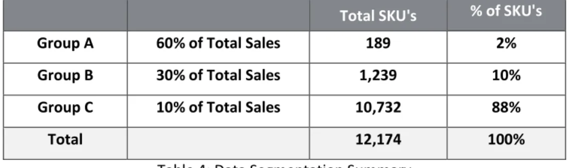
4.1.1 Data Segmentation Results and Discussion

In step 3 of our approach, we segmented the SKUs into three groups (A, B, and C) based on total sales volume over the most recent 18 months of data received from the Company. Group A were the SKU’s that contributed to 60% of total sales; Group B were the SKU’s that contributed to 30% of total sales; and Group C were the SKU’s that contributed to 10% of total sales. The results summary is in table 4. Product segmentation is used to prioritize products that contribute the most to sales and it helps companies develop inventory management approaches that allocate resources appropriately. For group A, we found that 189 SKU’s, representing 2% of the total SKUs, contributed to 60% of the Company’s cumulative sales. For group B, we found that 1,230 SKU’s, representing 10% of the total SKUs, contributed to 30% of the Company’s cumulative sales. For group C, we found that 10,732 SKUs, representing 88% of the total SKUs, contributed to 10% of the Company’s cumulative sales. We expected to see a similar distribution and the results confirmed our assumption that the Company had a few numbers of SKUs that were driving sales.

(27)

Page 27 of 37

Total SKU's % of SKU's

Group A 60% of Total Sales 189 2%

Group B 30% of Total Sales 1,239 10%

Group C 10% of Total Sales 10,732 88%

Total 12,174 100%

Table 4: Data Segmentation Summary 4.1.2 Data Integration Results and Discussion - Part 1

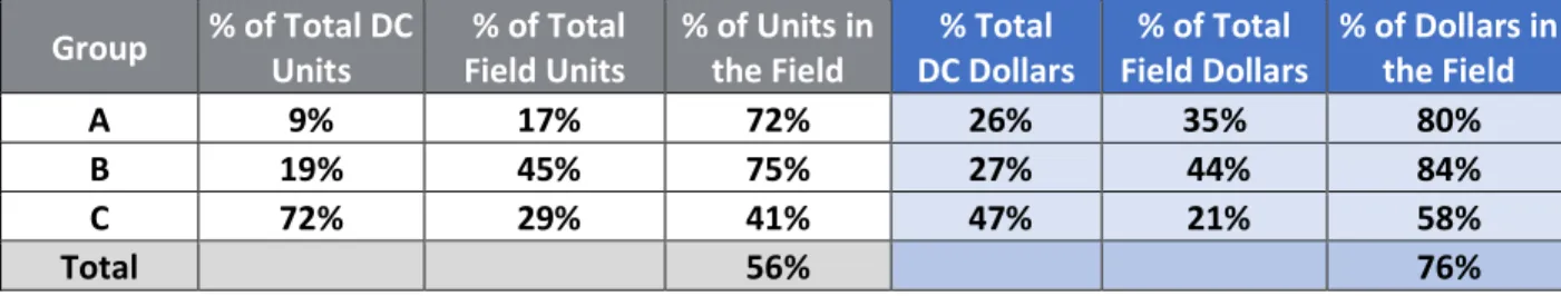
The Company uses internal inventory data to forecast their demand because they do not have access to real time field data from 3rd_{party distributors or hospitals. Once we confirmed the distribution} of inventory using SKU segmentation, we compared the total contribution of internal inventory to field inventory by units and value. The results by segment are in table 5.

We expected to have more inventory in the field on average when compared to what the Company held in their internal DC. When we compared the inventory in units, groups A and B had over 70% of their inventory in the field, confirming our hypothesis. Group C, however, in units, had over half of their inventory in internal DC locations. When we calculated the total contribution in dollar value per segment, we found slightly different and exaggerated results; groups A and B had over 80% of their inventory value in the field, and group C had over half of their inventory value now in the field vs internally. Group B, in both analyses had the largest quantity of inventory in units and value in the field. In total, 56% of the Company’s inventory volume was in the field, but that quantity contributed to 76% of their total value.

In summary, the Company held more inventory in the field than in their internal DC; the largest percent of the field inventory was from segment B; and the difference between internal and field volumes were not as great in units as in value. The Company cumulatively held 76% of the inventory in the field where they do not have product visibility. Based on this finding and understanding their limitations, which are their access to field data for forecasting demand, we wanted to compare the forecast accuracy between the segments.

(28)

Page 28 of 37

Group % of Total DC _Units % of Total _{Field Units} % of Units in _{the Field} _{DC Dollars}% Total _{Field Dollars}% of Total % of Dollars in _{the Field}

A 9% 17% 72% 26% 35% 80%

B 19% 45% 75% 27% 44% 84%

C 72% 29% 41% 47% 21% 58%

Total 56% 76%

Table 5: Data Aggregation Summary Part 1 4.1.3 Data Integration Results and Discussion - Part 2

From part 1 of the data analysis, we confirmed that most of the Company’s inventory had been in the field and therefore not visible when forecasting demand. Therefore, we calculated and compared the total order units and forecast error between each segment. The results summary is in table 6. As we expected, the forecast error variation increased from group A to group C, but unexpectedly, group B had the greatest order volume. This may be driven by the demand forecasting tool being fed more data points for the high runner SKUs which may have improved its forecasting accuracy performance. Further analysis is required to investigate this point.

To further understand the relationship between the forecast error and total order units, we calculated first, the potential lost dollars using the SKUs that were under-forecasted. Secondly, we quantified the inventory value that was in excess due to over-forecasting. A negative forecast error meant the demand was over-forecasted and a positive forecast error meant the demand was under-forecasted. The potential lost dollars and the excess inventory calculated were only estimated for purposes of showing the Company directional insight. The potential lost dollar estimates assume that the demand will not be satisfied elsewhere, and that the customer will wait for the product.

In the analysis, we expected group A or group C to be the primary contributors to their excess inventory. Group A SKUs were of higher value, therefore, we assumed that with a slight forecast error they would greatly contribute to the Company’s excess inventory problem or potential lost dollars; Group C, we hypothesized, would be the primary contributor to excess inventory due to pure volume. After calculating the potential lost dollars and the inventory value that was in excess, as we assumed, group A contributed the most to potential lost dollars. However, unexpectedly, group B contributed the most to the inventory value that was in excess. Of all the units ordered, the SKUs from group B were ordered more frequently and on average, group B had a forecast percent error of -18%. Due to the greater number of orders observed in group B, we believe the forecast variation in combination with product value and product visibility, may have contributed to this group being the primary driver for excess inventory.

(29)

Page 29 of 37

Group % of Total Order _Units _{% Avg Error}FCST Max FCST % _Error Min FCST _{% Error}

A 35% -2% 14% -36%

B 43% -18% 75% -234%

C 22% -28% 100% -75K%

Total

Table 6: Data Aggregation Summary Part 2 4.1.4 Tableau Data Integration Results and Summary

To further investigate the relationship between the sales and inventory volume, we used Tableau to visually display the volume distribution by the territory regions provided by the Company. The territory regions are where 3rd_{party distribution centers are located. The sales volume by region is displayed in} Figure 15 and the inventory volume is displayed in Figure 16. Comparing Figure 15 and 16, it appeared that while California, Virginia, Pennsylvania, Florida, and New York had the highest sales across the states, they were also among the top 5 states holding inventory volume.

To directly compare sales and inventory volumes by state, we created a graph to show the relationship; see Figure 17. Analyzing the data visually, as expected, there is a positive relationship between the states with the highest sale shipments and the states with the highest inventory volume. However, this does not necessarily correlate to the demand per state. The distribution of the inventory among the states is not directly proportionate with the volume shipped per state. For example, while Washington state is not on the top 10 states based on shipped-to volume, it is one of the top

contributors to the overall inventory, and the case for Virginia state is the opposite. This signals that there should be other underlying factor(s) that influences inventory distribution per state that requires further investigation.

(30)

Page 30 of 37

Figure 14: Inventory volume per state

Figure 15: Sales and Inventory Volume Comparison by State

4.2 Project Approach Considerations

The team believed that by connecting the data and enabling root cause analysis determinants, we could identify opportunities for the Company to use customer-centric data to reduce inventory or create other efficiencies. When we first approached the problem of excess inventory, we underestimated the amount of data we would need to work with in order to output valuable insights for the Company. When we realized the extent, we interviewed employees at the Company, who confirmed that they were unsure on how to approach “big data.” This element of “big data” is relevant in the supply chain industry and many companies struggle managing these data sets.

When we initially realized we needed to aggregate multiple files from various sources, we had yet to identify the need to use a programing platform like Jupyter Notebook. We came to this realization when we started to clean and try to transform the files manually. This was an impossible task with the amount

(31)

Page 31 of 37

of data we were given; the effort was too time consuming and had a high risk of human error. We realized that in order to complete any analysis, we would need to program code to clean, transform and integrate the files. Originally, we were going to use MySQL workbench, another open-source relational database system, but the MySQL workbench is not ideal when trying to analyze data in time series. Once we learned about Jupyter Notebook, the user friendly and recognizable platform, became our programing application of choice. Jupyter Notebook is commonly used for data cleaning, transformation, statistical modeling, machine learning and more. It also supports multiple programming languages like Python, and it reads and writes excel and csv files, all which were needed for the analysis.

4.3 Limitations

All the data provided was not collected in real-time; and therefore, the analysis does not represent inventory distribution today. The data analysis and recommendations are directional and provide a holistic picture of the Company’s inventory management. For this reason, the data segmentation and analysis were completed at an aggregate level, representing the last 18 months of data instead of drilling into the month by month data analysis. The ability to drill down into monthly time intervals is a recommendation for future analysis.

Another limitation is that the data was collected from various sources and there were product codes with missing data; for purposes of this capstone and its objective to provide directional insights, these product codes were removed from the data sets. Another important consideration was the extreme values in the demand file for product codes that were either under- or over-forecasted. An example of this was when the Company forecasted zero orders for a product code that had an abnormal order quantity for that month.

4.4 Alternative Methodology

To approach the original problem presented by the Company, we cleaned and transformed the files via Excel Workbook or Jupyter Notebook and then further analyzed in an Excel Workbook. An alternative method would be to use only Jupyter Notebook to clean, transform, and analyze the data. The company data was also aggregated by month into one data frame and the average for each product code was calculated for the analysis. An alternative method would be to analyze the integrated data without calculating the averages. This would require the analysis to be completed in Jupyter Notebook to handle the amount of data for large time horizons. For this reason, in future analysis, we recommend a shorter

(32)

Page 32 of 37

time horizon (only 3-6 months of data) is used to manage the data integration analysis with it captured in monthly time intervals.

Chapter 5: Conclusion

5.1 Insights and Management Recommendations

Our first set of insights relate to the impact on inventory due to forecast accuracy.

Insights 1: The following conclusions were drawn (as a reminder, the potential lost dollars and excess inventory dollars are estimations to show directional value):

 Group C had the greatest forecast variation and the largest bias as shown in table 7.  Group A is the primary driver of potential lost dollars, likely due to under-forecasting.  Group B is the primary driver for excess inventory in dollars, likely due to over-forecasting.

Due to the Company not having access to field data when forecasting demand, the forecast can only be controlled so much by using internal DC data. We believe this is contributing to the higher inventory levels we see in Group B.

Recommendation 1: Our recommendation to the Company is to further analyze the aggregated data sets to show the potential value of integrating data sources between third party distributers and the company. To determine that value, we recommend that the Company complete the following analysis using the aggregated data tool:

 First, complete a regression analysis to show correlation between forecast accuracy and inventory levels to determine the relationship function(y).

 Second, create a new forecast using 3rd_{party distributor data and sales demand.}

 Third, use the new forecast and perform a hypothesis test to show whether there is a significant difference between the new and old forecasting method. We hypothesize that there would be a significant difference.

 Finally, use the regression function(y) to project new inventory levels with new the new forecast method.

The new projection from the final step would be used as the value proposition when discussing future opportunities to share data with 3rd_{party distributers. As mentioned in the literature review, product} visibility is critical for creating an agile, adaptive supply chain.

Our second set of insights and recommendations relate to the analysis of the excess inventory. Insights 2: The following conclusions were drawn from the analysis on excess inventory: