Communication over fading dispersive channels.

DOCUM1ENT OFFCE 36-412

RESEARCH LABORATORY OF JIIEC1'RONICS SSACHUSSITFS INSITUE OF TECHNOLI0 Y

COMMUNICATION OVER FADING DISPERSIVE CHANNELS

JOHN S. RICHTERS

/

i· C ,vS,-

,

.?

f TECHNICAL REPORT 464 NOVEMBER 30, 1967

MASSACHUSETTS INSTITUTE OF TECHNOLOGY

RESEARCH LABORATORY OF ELECTRONICS CAMBRIDGE, MASSACHUSETTS 02139

The Research Laboratory of Electronics is an interdepartmental laboratory in which faculty members and graduate students from numerous academic departments conduct research.

The research reported in this document was made possible in part by support extended the Massachusetts Institute of Tech-nology, Research Laboratory of Electronics, by the JOINT SER-VICES ELECTRONICS PROGRAMS (U.S. Army, U.S. Navy, and U.S. Air Force) under Contract No. DA 28-043-AMC-02536(E); additional support was received from the National Aeronautics and Space Administration (Grant NsG-334).

Reproduction in whole or in part is permitted for any purpose of the United States Government.

Qualified requesters may obtain copies of this report from DDC.

MASSACHUSETTS INSTITUTE OF TECHNOLOGY RESEARCH LABORATORY OF ELECTRONICS

Technical Report 464 November 30, 1967

COMMUNICATION OVER FADING DISPERSIVE CHANNELS

John S. Richters

This report is based on a thesis submitted to the

Department of Electrical Engineering, M. I. T.,

August, 1967, in partial fulfillment of the require-ments for the degree of Doctor of Philosophy.

(Manuscript received September 1, 1967)

Abstract

The transmission of digital information over a fading dispersive channel is con-sidered, subject to a bandwidth constraint on the input signals. A specific signaling scheme is proposed, in which information is transmitted with signals formed by coding over a set of smaller basic signals, all of which excite approximately

inde-pendent and orthogonal outputs. The problem is then modeled as one of block coding

over successive independent uses of a diversity channel.

Upper and lower bounds to the minimum error probability attainable by such a

scheme are derived. These bounds are exponentially decreasing in terms of the

time available for information transmission, and agree asymptotically for a range

of rates. These bounds are used to interpret the significance of different signal

and channel parameters, and the interplay between them.

Some conclusions are drawn concerning the nature of good input signals, the major one being that any basic signal should be transmitted at one of a small

num-ber of discrete voltage levels. Several numerical examples are included, to

illus-trate how these results may be applied in the estimation of performance levels for practical channels.

TABLE OF CONTENTS

I. INTRODUCTION 1

1. 1 Communication System 1

1. 2 History of the Problem 2

1. 3 Summary of This Research 3

II. DIGITAL COMMUNICATION OVER FADING CHANNELS 4

2. 1 Channel Model 4

2. 2 Digital Communication 7

2. 3 Signaling Scheme 9

2. 31 Input Signals and Output Statistics 9

2. 32 Signal Design 12

III. BOUNDS TO ERROR PROBABILITY 17

3. 1 Expurgated Bound 17

3. 11 Equal Eigenvalues 19

3. 12 Zero-Rate Exponent 21

3. 13 Positive Rates 27

3. 2 Random-Coding and Sphere-Packing Bounds 41

3. 21 Zero-Rate Bound 43

3. 22 Positive Rates 47

3. 23 Capacity 47

3. 3 Comments 48

IV. RESULTS AND INTERPRETATION 51

4. 1 Discussion of Results 51

4. 11 Significance of p(x) 51

4. 12 Comparison with the Gaussian Channel 52

4. 13 Comparison with Orthogonal Signals 52

4. 2 Application to the Communication Problem 56

4. 21 Exponent-Rate Curves 56 4. 22 Zero Rate 58 4. 23 Capacity 60 4. 24 Other Rates 63 4. 25 Comments 65 4. 3 Numerical Examples 66 4. 4 Signal Design 71 4. 41 One-Dimensional Signaling 73 iii

_

C III

I __ __

1____1_

CONTENTS

V. SUMMARY AND CONCLUSIONS

5. 1 Summary 5. 2 Conclusions 5. 3 Future Work Appendix A Appendix B Appendix C Appendix D Appendix E

Conditions Sufficient for Exponent Maximization

Theorems Concerning the Expurgated Bound for Equal Eigenvalues

Theorems Relating to the Random-Coding Bound for Equal Eigenvalues

Optimality of Impulses

Lower Bound to Error Probability

Acknowledgment References iv 76 76 76 77 78 86 96 104 124 140 141 _ _ ___I

I. INTRODUCTION

Channels that exhibit both fading and dispersion are often used for communication

purposes. Perhaps the best known examples of such channels are fading ionospheric

radio links, and tropospheric scatter systems. More recently, communication has

been achieved by reflection from the lunar surface and through plasmas, and fading-dispersive channels have been artificially created as in the case of Project West Ford.

Our main concern is the use of such a channel for digital communication when the

input signals are bandwidth-constrained. We wish to obtain estimates of performance

for such a communication system, and to use these to determine how the interaction between input signals and channel statistics affects the ultimate error probability. Our

tools for this study consist of the techniques of communication theory and information theory, and we shall rely heavily on the use of bounds on the attainable error probability.

1. 1 COMMUNICATION SYSTEM

By digital communication, we refer to transmission of one of M equiprobable input 1

signals, at a rate R = -ln M nats/sec. The signal is corrupted by the channel, and we

choose to decode at the channel output for minimum error probability. We shall use the notation Pe to stand for the minimum attainable error probability, minimized over all sets of input signals and decoders (subject to such constraints as bandwidth, average power, etc.). We wish to determine in what fashion R and the channel characteristics affect P

e

We envisage the channel as composed of a large number of point scatterers, each with its own time delay, Doppler shift, and reflection cross section. Subject to certain restrictions on the input signals and assumptions about the scatterers, the channel characteristics may be summarized by the scattering function r-(r, f), where o-(r, f) drdf is the average energy scattering cross section of those scatterers with time delays between r and r + dr and Doppler shifts between f and f + df.

We consider constructing the M input signals by modulating N smaller basic

sig-nals designed so that each is independently affected by the channel (that is, no

inter-symbol interference or memory). Each of the M signals will consist of a set of N

modulation levels, one for each basic signal, and the problem then reduces to coding

over the N basic signal modulation levels. The bandwidth constraint enters into the

determination of N.

Such a model describes many actual systems for communication over fading-dispersive channels, although usually no attempt is made to exploit the possibilities of coding. For this type of scheme our analysis will provide ultimate performance limits. Moreover, our results should be indicative of the manner in which the signal and channel parameters interact for more general communication systems.

1

1. 2 HISTORY OF THE PROBLEM

There is a large body of previous work concerning this kind of problem. We make

no attempt to give a complete listing of results, but try to mention earlier work that seems most pertinent to the present analysis.

For digital communication, with specified input signals, the optimum receiver is

defined as the one that minimizes error probability. The determination of the optimum

receiver has been considered by several authors in recent years. Price,1,2 Price and

Green,3 and Kailath4 have studied problems involving M-ary signaling over Gaussian

multipath channels, and Middleton,5 Turin,6 and Bello7 have considered the

binary-signal situation. The result of these studies is that the form of the optimum receiver

is known (it can be interpreted as an "estimation-correlation" operation ).

Although the form of the optimum receiver for an arbitrary set of M input signals

is known, little can be said of the resulting system performance. For example, we

would like to vary the set of input signals (subject to the constraints), consider each set with the corresponding optimum receiver, and choose the combination that results

in an error probability smaller than all the others. This set of signals and receiver,

or decoder, would then be defined as the optimum combination for communication over

the particular channel under consideration. Unfortunately, because of the complicated

form of the optimum decoder, exact error probabilities have been calculated only in special cases.

There is, however, another method for attacking this problem, one that avoids some

of the complexities just mentioned. This method by-passes the exact calculation of

error probabilities in favor of the determination of bounds to the probability of error

that may be achieved by transmitting over such a channel. It is frequently possible to

derive upper and lower bounds to the achievable probability of error which agree

expo-nentially. For our purposes, this will be nearly as satisfactory as an exact error

prob-ability because our primary interest is not merely the determination of a minimum error probability but the study of how the interaction between input signals and channel sta-tistics affects the error probability.

These bounding techniques have been widely applied to discrete memoryless channels

(see for example, Shannon,8 Fano,9 and Gallager 0), and have recently been used by

Holsinger and Ebert12 to study the problem of communication over a deterministic

colored Gaussian noise channel. Pierce1 3' 14 has derived bounds for the binary case

with slowly fading channel and variable data rate, and for a special M-ary transmission

case with linear filtering at the decoder. Jacobs 15 first showed that the capacity of an

infinite bandwidth fading channel is the same as that of an equivalent Gaussian channel.

The problem considered here is quite similar to that analyzed by Kennedy,1 6 who

treated fading dispersive channels with M-ary orthogonal signals, and derived both upper

and lower bounds to the attainable error probability. There is one most important

dif-ference, however, in that orthogonal signals require a large amount of bandwidth, and

2

we assume that the input signals must be bandwidth-constrained. This turns out to be a major distinction, making the problem more difficult to solve, and in many cases, physically more meaningful.

The reader who is interested mainly in the nature of our results might choose at this point to glance at the first sections of Section IV, where some of the major points are summarized and discussed.

1.3 SUMMARY OF THIS RESEARCH

In Section II, we derive an approximate mathematical model of the channel, and dis-cuss the problems involved in using a fading dispersive channel for digital communica-tion of one of M arbitrary input signals. Then we enumerate several specific types of

signaling schemes, and mention briefly the problems involved in signal design.

Section III is devoted to determination and evaluation of bounds to error probability, by using the channel statistics derived in Section II. It is highly mathematical in nature and provides the abstract results necessary for the evaluation of performance levels.

In Section IV, we discuss the physical significance of the results of Section III, and relate these results to the communication problem set forth in Section II. We illustrate possible applications through some numerical examples, and return to the question of signal design.

3

II. DIGITAL COMMUNICATION OVER FADING CHANNELS 2. 1 CHANNEL MODEL

The problem under consideration is the transmission of information over a linear,

time-continuous, fading, dispersive channel. The channel is envisioned as a collection

of a large number of independent point scatterers, such as the ones that made up the West Ford belt, for example. Any input signal s(t) will be a narrow-band signal

cen-tered at some nominal high carrier frequency, o, so that

s(t) = Re u(t) e }, (1)

where u(t) is known as the complex lowpass modulation of s(t). By narrow-band, we

mean that the bandwidth of s(t) is much less than . Consider a particular scatterer

with range r sec and Doppler shift f Hz. If 2rrf << CO, then the signal returned by that

scatterer will be approximately

y(t) = Ree u(t-r) e[ ( )oo r]}, (2)

where A is an attenuation factor. It is unlikely that the value of r could be specified

within 2r/o sec, so that it is reasonable to consider the quantity 0 -wOr as a random

variable distributed uniformly over (0, 2).

Let us partition the set of possible ranges and Doppler shifts into small cells, and consider one particular cell centered on range r and Doppler shift f, containing a

num-ber of scatterers. If the dimension of the cell in r is small compared with the

recip-rocal bandwidth of u(t), and the dimension in f is much less than the reciprecip-rocal time duration of u(t), then the contribution to the total received process from all the scat-terers in that cell will be

y(t, r, f) = Re (r, f) ejo(r'f) u(t-r) e

}

(3)

where A and 0 describe the resultant amplitude and phase from all scatterers in the cell.

With a large number of independent scatterers in the cell, each with random phase and approximately the same reflection coefficient, A(r, f) will tend to have a Rayleigh distribution, while 0(r, f) will become uniform on (0, 2). 17 In that case, the real and

imaginary parts of A(r, f) ejO(r'f) will be statistically independent, zero-mean, Gaussian

random variables with equal variances. Note that the number of independent scatterers

in a cell does not have to be particularly large for this to be true; in fact, as few as six

may give a good approximation to Rayleigh amplitude and random phase. 1 8

With the previous assumptions, the total signal y(t) received from all of the cells for a given input u(t) will be a zero-mean Gaussian random process, and thus the

statistics of y(t) may be completely determined from the correlation function

Ry (t, r) = y(t) y(T). (4)

If it is assumed that scatterers in different cells are uncorrelated, and that the cells are small enough so that sums may be replaced by integrals, the expectation may be carried out, with the result that

Ry = Re (r) u() u(t-r) u*(-r) ej2 f(Tt) drdf} - (5)

The quantity -(r, f) equals A (r, f), and is known as the channel scattering function. It

represents the density of reflecting cross section, that is, (r, f) drdf is the average

energy scattering cross section of those scatterers with ranges between r and r+ dr sec and Doppler shifts between f and f + df Hz. If we assume that there is no average energy loss through the channel (this is no restriction, since any average attenuation may be accounted for by a normalization of the input signal level), then

S Sn

(r,f) drdf = 1. (6)

A typical scattering function is illustrated in Fig. 1. The most important charac-teristics of a(r, f) are B, the frequency interval in f outside of which o-(r, f) is

essen-tially zero, and L, the time interval in r outside of which (r,f) is effectively zero.

The quantity B is called the Doppler spread, and represents the average amount that an input signal will be spaced in frequency, while L is known as the

multi-path spread, and represents the average amount in time that an input signal will

be spread. Table 1 lists approximate values of B and L for some practical cases.

The exact way in which B and L are defined is unimportant, since these will only be used as rough indications of channel behavior.

( r, f)

Fig. 1. A typical r-(r,f).

5

Table 1. Values of B and L.

Channel B(Hz) L(sec)

Ionospheric Scatter 10 10 4

Tropospheric Scatter 10 10

West Ford Belt 10o 10

Chaff Clouds 102 5 X 10- 6

Moon Scatter 10 10 2

If -(r, f) is well-behaved and unimodal as shown, then an input of a single sine wave will result in an output whose correlation time or fade duration will be approximately

1/B sec; that is, the fading of any two points on the received process should be essen-tially independent if they are separated by 1/B or more seconds. If the input consists of two sinusoids, they should fade independently if their frequency spacing is at least of the

order of 1/L Hz. It has been shown elsewhere,l 6 that if the input signal has duration T

and bandwidth W, the received waveform will have a number of degrees of freedom (the total number of independent samples in the output process) approximately equal to

r(i+BT)(I+LW), if BL < 1 or TW = 1

K = (7)

(T+L) (W+B), otherwise

We emphasize the roughness of relation (7). The channel will later by treated as a

diversity channel with K paths, and (7) is used only to estimate K. The validity of this

channel model will not depend on the accuracy of (7), although any numerical results will be approximate to the extent that it gives a good approximation of K.

n(t)

st (t) - r(t)

INPUT

SCATTER

SIGNAL

ADDITIVE

TOTAL

SIGNAL

CHANNEL

PORTION OF

NOISE

OUTPUT

OUTPUT

SIGNAL

Fig. 2. The channel model.

We also assume that any signal that we receive is corrupted by the

addi-tion of additive, white, zero-mean Gaussian noise (such as front-end receiver

noise) with density No/2 watts per Hz. A block diagram of the over-all

chan-nel model is shown in Fig. 2.

6

2. 2 DIGITAL COMMUNICATION

The basic problem to be considered is digital communication over a fading, dis-persive channel, accomplished by sending one of a set of M equiprobable signals and decoding at the output for minimum average error probability, Pe. These input signals are assumed to be time-limited to (0, T), and we shall be interested mainly in the

asymptotic case, where M and T are large. We also require that the signals all lie

essentially within a bandwidth W, and that the average transmitter power be less than or equal to Pt. Ideally, our procedure would be to choose an arbitrary set of M input signals that satisfy the constraints, determine the optimum receiver for these signals, evaluate the resulting Pe' and then choose the set of M signals that result in minimum Pe for the particular fading channel under consideration.

The first step is to find the optimum receiver for an arbitrary set of M signals. This problem has been previously considered by several authors, with the result that

the form of the optimum receiver is known. Perhaps the simplest description is that

given by Kailath,4 who shows that the optimum receiver may be interpreted as a bank

of "testimator-correlator" operations. That is, one element of the receiver takes the

channel output, assumes that a particular input signal was sent, computes a minimum mean-square error estimate of the signal portion of the output (before the noise is

added), and correlates this with the actual output signal. Unfortunately, except in a

few very special cases, it is practically impossible to use the previous results for the computation of error probabilities for a given set of M signals, because of the

com-plicated expressions that must be evaluated. This is hardly surprising, for even in

the simpler case of the nonfading, additive Gaussian noise channel, exact error proba-bilities cannot usually be computed for large numbers of input signals.

In the case of the additive Gaussian noise channel, one approach is to use bounds

on Pe, rather than to attempt to compute actual error probabilities. This has been

done successfully by various authors,10' 11, 12 1 9 who have found upper and lower

bounds to Pe which in many cases agree very well for large M and T. This allows

one to design signals that minimize the bound on Pe' which has proved much simpler than the minimization of Pe itself, and yet has often yielded useful results. When a fading channel is considered, however, the more severe nature of the channel variations makes even computing bounds to Pe a major problem.

In order to illustrate the difficulties, and obtain results that will be useful later, we consider an input signal, xs(t), where s(t) is a unit energy signal, and x is an

amplitude modulation. It is possible to expand the output signal in a

Karhunen-Loeve orthonormal expansion,20 using the eigenfunctions of Ry (t, T) to obtain

00

r(t) = rkk(t) (8)

k=1

7

rk = r(t) kI(t) dt (9)

k APk(t) = 0 R0R(t, T) k(T) d. (10)

Properties of the solutions to the integral equation given in (10) have been enumerated

by several authors. 1 0' 11,12,19,21 If Wo is very large, it has been shown that the

eigenfunctions fk(t) will approximate conjugate pairs, with both functions of any pair

having the same eigenvalue. Thus, for any particular eigenvalue Itk' if Tk(t) is a

solu-tion to (10), then lk(t) is orthogonal to Ik(t) and is also a solusolu-tion. Moreover, it may be shown that

rirk (x k+ 1No) ij (11)

rirk = 0, (12)

provided the additive noise is white. Thus each rk is a zero-mean complex Gaussian random variable, and they are all statistically independent.

Because of our normalization of the channel and input,

o ₀0 o

2

k = E 1kk(t) 4k(t) dt Lk = X Ry(t,t) dt = 1. (13)

k=1 k= 1

For later convenience, lump each pair of tLk together and call the result kk' so that Xk=

2_{Bk; then, there will be half as many}

X's as 's, and

co

kk = 1 . (14)

k=1

Each Xk may be interpreted as the fraction of total received energy contributed by the

kth diversity path, on the average. The total number of significant k will be

approxi-mately equal to K, as given by (7).

If one of two input signals is sent, we can make use of the fact that any two

sym-metric, positive-definite matrices can be simultaneously diagonalized, 2 2 to find one

(nonorthogonal) expansion that results in independent components of r, regardless of which signal was sent. The eigenvalues will no longer have the same simple interpre-tation as before, however, and more importantly, if both signals are simultaneously modulated and transmitted, they cannot be separated at the output because they will

each excite the same output components and hence result in crosstalk. For M

arbi-trary signals, there is no one output expansion that results in independent signal

8

components, regardless of what signal was sent.

Due to the fact that we cannot separate the components received at the channel output from many different arbitrary input signals, the general communication problem seems insurmountable, at this time. If, however, we start with a set of basic input signals that can be uniquely separated at the channel output, with output components that are all statistically independent, then we could consider coding over this signal set and have

some hope of computing error probabilities. In particular, the problem could be

formu-lated as one of communication over a time-discrete, amplitude-continuous memoryless channel.

Unfortunately, such a restriction to a specific basic input set would preclude any general determination of ultimate performance limits. Coding over a specific set will certainly result in an upper bound to the minimum attainable Pe. Moreover, for reasons of simplicity, many existing fading dispersive systems employ basic signal sets of the type just described, and thus analysis would yield bounds on the best possible results

for systems of that class. Finally, an analysis of this type of scheme will still allow

us to obtain a greater understanding of the performance limits of bandwidth-constrained

fading dispersive channels than has been previously available. We shall return to some

of these points.

2.3 SIGNALING SCHEME

We choose a set of input signals that have the desirable properties mentioned above, namely a set of time and frequency translates of one basic signal, with sufficient guard

spaces allowed so that the output signals are independent and orthogonal. In the first

subsection we consider the output statistics for an arbitrary choice of basic signal and derive an equivalent discrete memoryless channel. In the second, some aspects of

sig-nal design are discussed. The problem is so formulated that existing bounds on error

probability may later be applied.

2. 31 Input Signals and Output Statistics

Consider a unit energy input signal that is approximately time-limited to Ts seconds

and bandlimited to Ws Hz, but is otherwise arbitrary. Time- and frequency-shifted

replicas of this signal with sufficient guard spaces in time and frequency left between

them will then yield approximately orthogonal and independent channel outputs. As we

have said, separating the input signals by more than L seconds in time will make the output signals approximately orthogonal, and an additional 1/B will make them inde-pendent, too. Similarly, in the frequency domain, a spacing of B Hz will make the out-put signals approximately orthogonal, and an additional 1/L will make them independent. We take our basic input signals to be the (say) N time and frequency translates of the given (Ts, Ws) waveform that satisfy these independence and orthogonality conditions

and exhaust the available time-bandwidth space (see Fig. 3). The outputs resulting

from these N basic signals will be independent and orthogonal.

9

W

BAN DWI DTH

. * 0

TIME

Fig. 3. Basic input signals.

Suppose we construct our M input signals by simultaneously amplitude-modulating

the N basic signals. In this case, the mth input signal may be expressed as x =

th -m

(xml xm2, . ,mN ), where xmn is the modulation on the nt h basic signal. Since each

basic input signal is assumed to have unit energy, we require

M N

M ~ E Emn TPt, (15)

m=1 n=1

in order to satisfy the average input energy constraint.

Consider one basic signal, with scalar amplitude modulation x. This is just the situation that we considered in section 2. 2, and the resulting output random process r(t) may be transformed into a vector r, whose components are statistically independent, zero-mean, complex Gaussian random variables. The kth component of r may be split into its real and imaginary parts,

rk = rkre + jrkim ' (16)

where each part is a real zero-mean Gaussian variable with variance1 (x2Xkk+No), and

the two are independent, so that

10

_

I_

___

C

[II

ii

1 rkre + rki

(rkre,rkimlX) = exp

(

. (17)

2 2

The components of rk enter the density in the form rkre + rkim, so, for the purpose of estimating x, it is only necessary to record this sum, and not the individual terms.

Define

1 = (kre2 +rim ) ₍₁₈₎

Yk N k

o

then it can be shown2 3 that

Ix) = (l+x 2 k/N - exp 1 + 2 k ). (19)

Recall that the properties of Xk ( l, k 2,... K) depended on the assumption that the

channel was lossless, and that any average attenuation should be absorbed into the

energy constraint. From (19), we see that No can also be absorbed into the energy

con-straint, provided that we redefine the constraint on the input to be

N M

M X x mn N* (20)

n=1 m=1 0

The quantity P is the average output signal power, and the value of xmn in (20) is

/ t times the actual channel input signal level. Now

P(Yk Ix) 1 exp

1 + X k so that the density

K

Plx) _{P(Y IX) k=l} II

exp

9, (21)

(22)

governs the output vector y, given x. Note that y is a sufficient statistic for the

esti-mation of x, and is thus all the receiver needs to record.

Until now, except for noting the over-all power constraint in (20), we considered

transmission of one amplitude modulated input signal, modeled as one use of an

amplitude-continuous channel. Since the N basic signals were chosen to be independent

and orthogonal, this is easily generalized to simultaneous modulation and trans-mission of each signal, thereby reducing the problem to N uses of a memoryless,

11

amplitude-continuous, time-discrete channel, where on each use the input is a scalar x, and the output a vector y.

Let Tg and Wg denote, respectively, the guard space between adjacent signals in

time and bandwidth. Then it is easy to see that

N TW (23)

(Ts+Tg) (Ws+Wg)

The rate of information transmission is usually defined as

R - T in M nats/second (24)

but the rate that will prove most useful in Section III is

RN - N In M nats/channel use. (25)

The energy constraint may be written

N M

mn

Na

(26)

n=l m=1 P

a N (T s+Tg) (Ws+Wg). (27)

As we have noted, the number of positive k will be approximately given by

(l+BTs)(l+LWs) if BL < 1 or T Ws = 1

K =

f(Ts

(28)

+ _{L)(Ws+B), otherwise}

Note that, as W goes to infinity (the bandwidth constraint is removed), a will go to zero,

provided Ts, Ws and the guard spaces are kept finite.

2. 32 Signal Design

We consider now several obvious questions that arise with respect to the signaling scheme just described. The N basic signals were chosen to be time- and frequency-shifted replicas of one original signal, and we could conceivably do better by using the same type of time and frequency spacing, but allowing each of the N basic signals to be different. Before evaluation of Pe,' this question cannot be answered, but it seems likely that nothing would be gained by such a scheme. For our model, the density

p (y lx) will be the same for a given input signal, no matter how it is shifted in the

allotted T, W space. Thus, if a basic signal is in some sense "good," it should be

"good," no matter where it is placed in the space. If we find one "good" signal, then we can make them all as "good" by replicating the original in time and frequency. This

12

is quite vague, but in Section IV we shall present some results that reinforce these statements. In any event, it is clearly a simpler mathematical problem to consider just one X in place of a set of vectors, so we shall continue to suppose that the N basic sig-nals all have the same p(ylx).

When the basic signals are all replicas of one signal, what should that signal be? Referring to Eq. 1, we are free to specify u(t), but it appears in the analysis only

through Ts, Ws, and X. Although Ts and Ws can usually be satisfactorily defined for

reasonable signals, there is no simple relationship between u(t) and ; indeed, finding

X, given u(t), consists of finding the eigenvalues of an integral equation, in general, a very difficult problem. The inverse problem, of finding a u(t) that generates a

particu-lar , is even harder. Since X is the important quantity in the mathematical model,

one reasonable approach would be to find the "best" X, Ts, Ws, and ignore the problem

of transforming X into a u(t). This would provide a bound on the performance of this

type of system, and would give systems designers a goal to aim at. For further dis-cussion of this problem, in the context of an orthogonal signal, unconstrained bandwidth

analysis, see Kennedy. Even in this simpler case, however, no definitive answer to

this design question could be obtained.

In Section III, when we compute bounds to Pe, it will develop that there are

formidable mathematical obstacles to evaluation of the bounds for arbitrary , so even

this approach appears to be lost to us. In the infinite bandwidth case, however, it was found that equal-strength eigenvalues, where

1

kk- K' k = 1, 2,..., K, (29)

minimized the bound to Pe, and in that sense, were optimum. Furthermore, by varying

K in an equal-strength system, a good approximation to the performance of a system

with arbitrary could often be obtained. When X is given by (29), we find2 3 that

K

PX(y/x) = (1+x 2/K)- K exp k= (30)

1 + x2/K K

Thus y = Z Yk is a sufficient statistic, with conditional density

k= 1

K-1 / YK

y exp_

PK(Y1x) = K (31)

r(K) (+x /K)

Therefore, in the special case of an equal-eigenvalue signal, the channel model becomes scalar input-scalar output. Note that if K is presumed to be given by (28), the

speci-fication of Ts and Ws provides a complete channel description. These are compelling

reasons for restricting the analysis to equal eigenvalues, but in Section III will be

13

kept arbitrary until the need for (and further justification of) the equal eigenvalue assumption becomes apparent.

One other question can be considered at this time. We have remarked that T should

g be at least L + 1/B, and Wg should be at least B + 1/L to ensure orthogonality and

inde-pendence at the output. In some instances, this can result in a large amount of wasted

guard space. For example, if B (or L) becomes large, an input signal will be spread a

large amount in frequency (or time), and a large guard space is required to separate adjacent signals at the channel output. On the other hand, if B (or L) is very small, there are no orthogonality problems, but a large guard space is required to obtain inde-pendent output signals. In the former instance, there is no obvious way of circumventing the need for guard space, in the latter there is.

In particular, one can artificially obtain independence by means of scrambling.

Con-sider several sequential (in time) uses of a (T,W) block of signals. We could now use

up any guard space resulting from the 1/B and 1/L terms by interleaving signals from another, or several other (T,W) blocks. Thus, signals could be placed in a (T,W) block with guard spaces of only B in frequency and L in time, while independence can be

obtained by coding over signals in different blocks that were all independent. Thus for

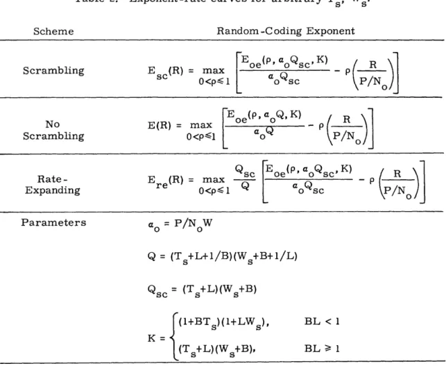
the same rate R, given by (24), the coding constraint length, N could be increased to TW N = (32) (Ts+L) (WS+B) while N sc M x - < a N (33) M mn sc sc n=l m=l P asc - N W (Ts+L)(Ws+B) (34) o 1 RN N InM, (35) Nsc Nsc

which would allow (we expect) a decrease in error probability.

Of course, we have in a sense changed the problem because we are no longer coding

over a block of (T, W), but over several blocks. While this should be a practical method

of lessening the guard-space requirements, it is not applicable to the problem of using

one (T, W) block for communication. We shall outline a "rate-expanding" scheme that

does not have this drawback.

In one block, there will be N (given by (23)) basic signals whose outputs are

inde-pendent and orthogonal, but Nsc basic signals whose outputs are orthogonal. Thus if

we packed in Nsc signals with Tg = L and Wg = B, there would be Nsc/N a sets of

N basic signals, where

(Ts+L+1/B)(Ws+B+ 1/L)

(36) (T s+L)(Ws+B)

The elements within any one of these sets would be orthogonal to and independent of each other, but the elements of different sets would, in general, only be orthogonal, not

inde-pendent. But if N is large, we expect reliable communication when any set is

trans-mitted, so we could consider sending information over all sets simultaneously. This

would increase our data rate to

R a R,

where the constraint length N is again given by (23), and now

N M M, 1 n=1 m=l (37) (38) x2 Na = N) mn re a

If Pe is the average error probability for one set (with constraint length N), and Pre is the probability of an error occurring in at least one of the a sets, then if Pe is small,

P aP

re e (39)

Since we expect Pe to be decreasing exponentially in N, the difference between Pre and

P _e should be negligible.

Xml

I

K

I

K PATHS N USES

XmN

I

K

Fig. 4. Equivalent diversity channel.

15

l

__II_

_I

___

I·___II__IY______Il___lrl-1-1111

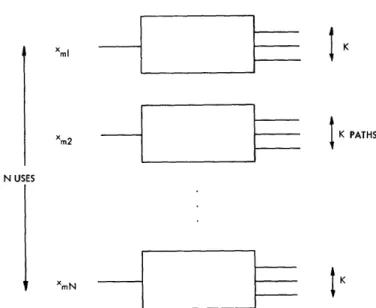
I_-The model just derived may be considered as N independent uses of a classical th diversity channel, with K equal-strength paths, as illustrated in Fig. 4. When the m code word, consisting of xm = (Xml,Xm2,... xmN) is transmitted as shown, each input component will excite K independent, identically distributed outputs, which may be summed to produce a random variable y, governed by the conditional density function of (31).

The description of the channel and its use just presented is, to be sure, an approxi-mate one. This has been necessitated by the complex manner in which the channel oper-ates on the input signals. We once again emphasize the roughness of the characterization

of (r, f) by just B and L. Although this may be reasonable when a-(r, f) is smooth and

concentrated as shown in Fig. 1, if cr(r,f) is composed of several disjoint "pieces" (typical for HF channels, for example), such a gross simplification obviously omits much information about scattering function structure. We shall return to this point in Section IV.

On the other hand, this channel model is essentially a simple one (particularly when the equal-eigenvalue assumption is invoked), and for the first time, provides an explicit

means of taking into account a bandwidth constraint on the input signals. We shall find

that this simplified model will still provide some insight into the communication prob-lem, and a useful means of estimating system performance.

16

III. BOUNDS TO ERROR PROBABILITY

We consider block coding over N uses of the amplitude-continuous, time-discrete channel model derived in Section II. We discuss both upper and lower bounds to Pe, the minimum attainable error probability, making use of many results presented in

Appendices. Each bound is found to involve an arbitrary probability density function

that must be chosen so as to obtain the tightest bound. The central problem considered

here is the specification of the optimum density and the resulting bound. The expurgated

random-coding upper bound to error probability is presented first, since it is func-tionally simplest and yields results that are typical of all of the bounds. Then the stand-ard random-coding upper bound is discussed, along with the sphere-packing lower

bound. These two bounds are found to agree exponentially in N for rates between Rcrit

and Capacity, and hence determine the true exponential behavior of Pe for that range of rates.

Some novel aspects of the present work should now be noted. The optimum density

just discussed consists of a finite set of impulses. This corresponds to a finite

num-ber of input levels, an unexpected result for a continuous channel. The normal sphere-packing bound cannot be applied to a continuous channel because the number of possible

inputs and outputs is unbounded. For this channel, however, the optimality of impulses

allows derivation of the lower bound, although with extensive modification. The results presented in this section are in terms of quantities defined in Section II, plus an

addi-tional parameter (p or s) that simplifies the analysis. In Section IV, these parametric

results will be converted into forms suitable for obtaining performance estimates for some practical systems. The reader who is mainly interested in the applications may skip to Section IV.

3. 1 EXPURGATED BOUND

Our point of departure is the expurgated upper bound to error probability derived

by Gallager. That bound is directly applicable only to independent uses of a

contin-uous channel whose input and output are both scalars. The generalization to a scalar

input-vector output channel such as the one considered here, is straightforward (for

an example, see Yudkin 24), so the details will be omitted. When applied to this

channel model, the bound states: If each code word is constrained to satisfy

N 2NRN

x Na, then for -any block length N, any number of code words M = e any

mn 2

p a 1, r 0, and any probability density p(x) such that f; x2p(x) dx = a < o, there exists

a code for which

P < exp - N{[p, p(x), r]-P[RN+AN]} (40)

O o r(- 2a+x 2 +x 2 )dxdx

ex[p,p(x),r] = -p n p(x) lx) e e xp(x H/ dxdx (41)

17

(l+kx2)

1/2 (l

2

)l/2

1x

HX(X,X1) = p(YX)1/2 P0(YJx)/2 dy = Xx1 ( (42) k=l 1+ 2 k(x+x) 00 1+X x k=1 1+ +kx 2 3

where the quantity AN -- as N - oo, provided f0 p(x) Ix2-a 3 dx < oo. All of the

proba-bility functions to be considered here will satisfy this constraint, so if N is large, the

AN term can be neglected. This parametric (on p) formulation of the bound is the usual

10

one, and the reader unfamiliar with its properties should consult Gallager. We recall

00

that k > 0, Z kk = 1. The difficulty lies in determining the r, p(x) combination that

k= 1

results in the tightest bound to Pe for a given X, p, a, that is,

Ex(P,a,X) =-p n min i0 p(x) p(x₁) e( I H(x,xl) /p dxdx₁j,

Lr, p(x) ]

(44) subject to the constraints

r > O0, p(x) 0, p(x) dx 1, p(x) dx = a (45)

In general, it is possible for a number of local minima to exist, so that the problem of minimizing over p(x) and r is a difficult one. Fortunately, for the particular channel

model under consideration here, H(x,xl) / P is a non-negative definite kernel (see

Appendix A, Theorem A. 2, for a proof), and these possible difficulties do not arise. In Theorem A. 1 it is shown that a sufficient condition on r and p(x) to minimize

S

O o _{p(x) p(x}r( 2a+x2+x2

1) er H(x,x1) 1/p dxdx1,

subject to the constraints (45) is

00

r(x2+x 2 00 r x2±x 1

p(x 1 ) H(xl/P d p p(x) p(x (l) e H(XXl)(X x 1/ dx

(46)

for all x 0, 0 < p < o, with equality when p(x) > 0. At this point it is possible that (46)

may have many solutions, or none but, because of the sufficiency, all solutions must

18

result in the same (maximum) value of exponent for the given X, p, a. It may also be shown that condition (46) is necessary as well as sufficient, but the proof is lengthy and tedious. Since we shall later exhibit solutions to (46), we can afford to dispense with a proof of necessity.

Unfortunately, the determination of the p(x) and r that satisfies condition (46) is a very difficult matter. In practice, the usual method of "solution" is to take a particular r and p(x), and plug them into (46) to see if the inequality holds. If it does, then r, p(x) solve the minimization problem for the p, a, X under consideration. We are now faced with the prospect of doing this for arbitrary X, for all values of p and a of interest.

Since the purpose of this study is to arrive at a better understanding of communica-tion over fading channels, it is worth while to make use of any reasonable approximacommunica-tion that simplifies the analysis. Even if the most general problem could be solved, it seems likely that the essential nature of the channel would be buried in a maze of details, and one would have to resort to more easily evaluable special cases in order to gain insight into the basic factors involved.

3. 11 Equal Eigenvalues

The simplest possibility to consider is that of equal eigenvalues, 1

k = -k k= 1,2,...,K. (47)

In this case, define

ErKn pX x pX1 r( 2a+x +x) H(XX /P dxdx

Exe(P, a, K) _=-p n ,p(x) in P P0 H(Xl)P dxdx (48)

HK(x, x1) = ( K)_1+ _ 1

1 + K (x+

, (49)

where r, p(x) satisfy constraints (45), and the subscript e denotes "equal eigenvalues." A simple change of variables proves that

Exe(P,a,K ) = K Exe ' K' (50)

Thus, as far as the minimization is concerned, we may set K = 1, compute Exe(p, a, 1),

and use (50) to obtain the result for arbitrary K. The only change is that we must loosen

the range 1 p < o to 0 < p < oo to allow for K > 1. This involves no additional effort,

since our theorems on minimization are valid over the whole range 0 < p < oo. Thus, when the eigenvalues are equal, X may be completely absorbed into the parameters p and a

19

___II_ _IPC----IIIIIII I 1-1- 11_111411 11 I_ 1 ·11_1_1

for the purposes of minimization on p(x) and r, a pleasant bonus.

As we have mentioned, this simplification is a good reason for restricting the anal-ysis to equal eigenvalues, but in addition, Theorem B. 3 in Appendix B states:

1, (51) where o00 b - k 2 (52) k= 1 00 d X3 (53) k= 1

and inequality (51) is satisfied with equality for any equal eigenvalue system. Thus, an

exponent that results from arbitrary k may be lower-bounded in terms of an exponent

with equal eigenvalues, thereby resulting in a further upper bound to Pe. This bound

is very similar to one derived by Kennedyl 6 _{for the infinite-bandwidth, orthogonal}

sig-nal case. The b2/d multiplier on the right-hand side of (51) may be interpreted as an

efficiency factor, relating the performance of a system with arbitrary eigenvalues to that of an equal eigenvalue system with an energy-to-noise ratio per diversity path of

ad/b. The orthogonal signal analogy of this bound was found to be fairly good for many

eigenvalue sets, thereby indicating that the equal eigenvalue assumption may not be as restrictive as it may at first appear. In any event, with equal eigenvalues we may set K = 1, and condition (46) may be simplified and stated as follows:

A sufficient condition for r, p(x) to minimize

r(-2a+x 2+x 2) /

Jo Jo

p(x) P(xl) e H1(X, xl)l/p dxdx Il, subject to constraints (45), is r x2+x2) 000 rx 2_{+x 1 /}

0

P(xl) e I Hl(X, xP) /dx s p(x) p(xl) e H1(X,xl) dxdxl (54)

for 0 < p < oo, with equality when p(x) > 0. In Appendix B, Theorem B. 1, it

is shown that, if r, p(x) and rl, Pl(x) both satisfy (54), then r = r, and

20

_ _ I_ __ __

-1 b2 b 3 = /b 2

E x(P, a, ) -_Exe d a V

0 px] dx =

S0

[p(x)-Pl(X)2 dx = 0, (55)

so that for all practical purposes, if a solution exists, it will be unique.

We shall digress and consider the zero-rate exponent, attained when p = oo. The previous results are invalid at this point (although correct for any p < oo), so this point

must be considered separately. We choose to do it now because the optimization

prob-lem turns out to be easiest at p = oo, and yet the results are indicative of those that will be obtained when p < o.

3. 12 Zero-Rate Exponent

When the limit p - oo is taken, it is easy to show that r = 0 is required for the

opti-mization, and

Ex(oo, a,) = -min p(x) P(x ₁) ln H(x,x ₁) dxdx₁ (56)

00

Ex(o, a,) = -m x in o p(x) p(x₁) ln H₁(xNk, x1 k) dxdx. (57)

p(x) k= 0

In the equal-eigenvalue case,

I00 .O00

Exe(O, a, 1) = -min

p(x) o o

p(x) P(x₁) n H₁(x,x ₁) dxdx₁,

where now

E(ooa,K) K) KExe(, Exe .K

We may change variables in (57) to obtain

00

Ex(oo, am) -min q k(x) qk(X) ln Hl(x, xl) dxdxl,

p(x) k=l

where qk(x) 1 p= _x , a probability density function with

§

x qk(x) dx = akk.

(58)

(59)

(60)

(61)

The minimum in (60) may be decreased by allowing minimization over the individual qk(x), subject to (61), so that

21

--- I I- I~~~~~~~~~~~~~~~~~~~~~~~~~~~---

~~

l~---rr~~ ll--- I(--~~-rc

~~

---

~~C---·--·~

-

00 00

E(oo, a,) - min qk(x) qk(Xl) In Hl(x, x) dxdx1 = Exe(0o, ak, 1)

X k- i q(x) 0 k1) 1

(62)

with equality when X consists of equal eigenvalues. This, together with (51), shows that

00 2

E x(0- abd, 1) Ex(o, a,) E a, 1) (63)

d x Exe(3

k= 1

with equality on both sides when X consists of equal eigenvalues. Thus at zero rate,

we have upper and lower bounds to the expurgated bound exponent for an arbitrary

eigen-value channel in terms of the exponent for a channel with one eigeneigen-value. Of course, at

this point, before evaluation of Exe (co, a, 1), we do not know how tight these bounds are. The derivation of the conditions on the p(x) that optimizes (56) is complicated by the fact that n Hk(x, Xl) is not non-negative definite. The derivation, however, only requires that n H\(x,xl) be non-negative definite with respect to all functions f(x) that can be represented as the difference of two equal-energy probability functions. In Theorem A. 2

it is proved that this is indeed the case. Utilizing this, the same theorem states a

con-dition on p(x) sufficient for the maximization of Ex(o, a, X). When simplified for one

eigenvalue, this becomes a sufficient condition for p(x) to optimize E xe(o, a, 1), subject to constraints (45):

S

p(x1) n H1(X,X l) dx1 > i

5

p(x) P(x 1) n Hl(x,xl) dxdx + o(x

2

-a) (64)

for some Xo, with equality when p(x) > 0. We dispense with the question of necessity,

since we shall now exhibit a p(x) that satisfies the sufficient condition and thus maxi-mizes Exe(00, a, 1).

In Theorem B. 2, it is shown that the probability function

p(x) = P1uo(x) + P2Uo(X-Xo) (65)

satisfies condition (64) for all a when the parameters pi, P2, and x are correctly

chosen. Therefore, at zero rate, the optimum p(x) consists of two impulses, one of

which is at the origin. In Appendix B, expressions are presented relating pi, P2, and

2

a as functions of x . This was done because it was simpler to express the results in

o

terms of x instead of a. Here we return to the more natural formulation, and in

Figs. 5 and 6 we present graphically the optimum distribution in terms of a. The

1

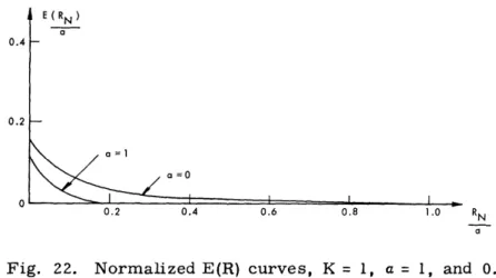
resulting exponent is presented in Figs. 7 and 8. Note that E xe(, a, 1) is a decreasing

function of a, and so

E e(oo, a, 1)lim E (0 a, 1) E 0. 15. (66)

a e a-0 a xe 00

E2EEE -f--*~ a -Z z 2 Z - --O 0 '-4 a '-4

6

cu ci_N. p- c Lt J½ 1J) 2 1-I iili I I I! 0 '-4 %D

p-;I I I I ..I I

. . . .. .

~.

. . . .I I - I . . I .. . . . 23 Cal-M~i - =1 I --- t -;t-- --I--- ·--I ·- --- --- ·--Y-·---L··---·--- ___ _ I I I ---,71 P--1-= EE I II i v co d

~-~4FI

=r--l~ffF -F11 = n. _{' -} a:l I V-dI C i= T-Ezif-l . #7

0--W~_

, -

-

iu-

.

-

.- ,

a m

WW

brt S

~

_L.t.-t-.-, 7 - -.

't---p

- t- :i..:t. X .=

. ZZ-

*- -1-4:F-

=-_=

4-Z.-

:

t : '-- _.-.

grK ,,,,

~~~47-.7,

.t_-

t-v<--I~Ii,\ 'T-t-F¢' g

4 It

v

~--8~--*-

+ r

<

-r:;:Z:

t

'1 ----

tfL

-er

~~~~~t.

W2h 4X

_

-l- -:- -t--_ ---

g7

.s_

--

.-

r.s--;--t

Z

tr =_

_

~

--

t}--1-

---^-Z--7

Zf e-+--;ELS°-.Z-|-.-i= I

*.

V -t -rg-

i--t--f---|-

- -- -- ;-

*'

. :~-t-: :I

,,

_{.'.i.t.t= -1-.t}

w

t¢*

_{t -~_t- *t}

1

+tt_-1

_{1:t t- .:}

.:-: .t: -74:::-l

_r::~

~

~

,,

¼1

t§i

[i .i;,t~tt-t~

Xr~_+-'4.-t-

V--4

ct~f.-t.m

~1tro

srL L '_G

LI i

Lifit

bt

h7fw\

w~

'I<I .II' 2..LLJ!2I11 I L ] ..

0 Hi L-:- iE---i L !j --Ee----t _ E L. tr I_. i f'_= t-4 ----' t: -- t ' :,f -' ' t . -H -Si F-+t---'r .'- 4-- t --N --l D iLL; L--L- ,:f-_rf :t- - .: . [rrg-g 4=i--EF 'I:.. ¢:ELL; -t.-;er..t--. .t48' -St+ :.H il f _f_...t: -.. t--.. : = t i- Tt;- i r -t -r b.- 1i---L -'--.L-.=.-S C-.t=-, -- i-- L-^ t -t=r-- ;- -- t-: s .t, .t .., . f -, r. =- a:. {_=$_ t f_., -t_,'._,-'- :r-:-s.--C t- L:-} -.; t .i_ t +._ t.:..ti_ ,F--t---t--,--i t-t: |- I4+- I + I i -e F->-t-,

t-t^-ttr;1 t t t -i r t t t tt - ---t --E-:t t:44-3-t~ ;t-x --- i;- -i

k.

T -=-f - '. ED -,,4:\- _ -t :.. -F -<--- T. - Lr- - -:, _ -= f:t- --- :|: 4 :! -= -. ._=t -_+;_ .'

t i - 4 7

.

3. -

t --1- =~~~~I

t

..._

_

t

=

._

* _

t==_

t ....- I _._ _ g - - --: t-- -T -' 1-' .1.==--F-E -T"' -- L-.t ,0__ :t:-l Tt t+. , -e-. -. t_ -= 2-X, t ._, f -_ , f -- - ----t _- --W. _,_ , .4;_ _: S:=S r S , .--1-._ ,¢_g tS:z:L 'E I ' i I I I I

iVXhi

6 .-il-) 0 .0 )H 0 H4 1 'lI H 0 H-N 0 H-'-4 24

K'_

,_

F L '

X

w

f W _

K

I" 'L x O -I t fall 7 1. |:z: . _ .i _E t~ '

-h

i: I . ta-#4r _{#11j ,._} -44 'tn-L : - -- .-,:: H -- I -- I E:4- -, T IF #I-- I:--L - -+ 7 -.- -f# :- Ali: -t''i _r ,L

T-1

I I I j " . t, , ,!j , 1 , I VI III J IW I,! 1 : I I 1-1 .-L a II :ii q I

'- ar- I- - -= =-_- r· _ -r ==_ A_ _ 1_ -- _ v-_ -- - 1 : -- --. F _= _LH=

-- t

1,=~~~~--- '1,=~~~~---1,=~~~~---1,=~~~~--- kl- s; 'ttH -- t -- -'W i' ·-= r- F--- -I~r--- -.-;- ---- -- Ir; r j-2 ?--i.. S.. -- --- _I Llr =--f I_._ _{- ---- ---·} --- --·- _.------·--- _{c - ·---. ·--} --- --- ,.i ._..._ ; -· ---- -·--- t: .. .. - ---_{.-._. .-.. '-- --} --'--- --- --r--c _{.-- r,r----c---i.-} .---.- c-.----..x---.-t-L.-.---- _---- -i---t---·--- _{--- .1: __} -- --I-i' --- L=l ----'E----· ---- r-.... ,..i "' "--- _::: L:T ----·--- .- ... _ --r-- ·- r-f---- --·--- ·---- ·- ·--- ·- --- 'CC _{r=-rl T-f=l--f}

i-l---L -ilec-rLL-ii-)---*

i---L---L-*-i-Lulil ·- ---i-

-W~~~~~~-

-

i.~~~~~Z

--

d C-t-S

-1 4

-7tT W_:_

i~l=ii

k I,

- i i ~~ ,d-=f ==t =': -J l, , , ,_,. . .-- Z: r .. .--,- . ,q_ _ ~ F _~T -'F

~rT ~.!,,-ili

-Tf.--~l(r;

~T:'

,i ~ r~ l !''L l'.]_-'r !" ,!,1' ~ ULE-2 _,~ .rq

-,

- _L . -r -- -, +: - --' _- _ .- -- - _- _ ... _{- -r--r-} .. _{mtl=+- _Ui} ': .~ itI!!il~L I

W1-Fit-S* L +

S' [ X

-->>~>-w--F~

lI -- t_-F~~~ t V-

-=>==->~~~~~~~~~~~~~~~~

-

> e

1

--L---. · --- ---- r --. - ii.-i.- -. -- ----. --t --.- -- -*--· · · - --- · -· --- ·- tT r ,r .. r. ,r -r i- :- iZZ c r --1 I L( i -- " c I+-L - I--C t c ?,.it-. i ' tt -Ciit Wri;Mh --N7 x ,2f~if~-+t,t ,t t,,H.' H ., , .. I 4 t ' ' --1 ' -'4 -tL:...Ft i ' -- - j- t$ti-.t -E -e~i'' LL tA' ' ' ,'C _ _ e.C ;- t; L·t*:'ti; 7 :¢_f dT±- IF 4-4-I + _ N i1 T ?/ L :

I-

.-4 4 -4 !I '4+- -t+ t -. _ = _ T r --" -+ _f =7j = -Tql + mr +iH4+ -' ' 44- 4L '' 'jt 1 -,- -I ;. | I . t-,1.-.- 1 ,F----i;t.-- ^.2 X _ - i _ r l t I _ I 1 ;-k.trs E } __ t i ji, j L- . 1-. r L m- 2.k. 1 -l L .. i -.; I _rW. t-t- -L :H , _ r; *t _-, _ ,e , H S e -t1W44-; r,--44 i

-4

-t 1- ,LT 4-f :, f -i44 -tt t .t itit ,Lt' H1 -12 4+ 0 04 25

-Ir1

4LI

-4-- I -IF -4 1Ti Li 41 . .J.

-

4

f 4 . --

t-~t

. _ >f '. F-:='1 - - -I -- --1 4 ... 7L -:----' t r r

f

E

ri -4- ;

1

-r;s-r I ., -_ ._ _7d -'1- r--=--· - = =-q . .-X- f.. = r =tL --0 H N 0 H o '---I

~

¢ -I.I 0 01 _r 14 bS *? ?~ 1_q 0 t:-' j-tLiL ji -fl '

tTir.·---L-_

_·I

i- ---- - -r '','; tcf H -I

¢!

I __ __j_ i .. " -:rt --- --- ·--- ·---·- ---- ---- _--

----

I---.. _{--·--- --- --- :-F;:} -- ---- r y t -- .... -- -L t- t L-L _--- --f.-l--

i ·_-·

C- --- i -i-· =L'f-

·---·- -· -·--i IfZLE7 --;L =r;- 4-i ·---L- _{--r- - -1-·-·} -- ii __ _:T-·- ___--- ----.... _ --L; -- --- --- - '-' i---'- t--- --- · --rL -t ---c- c.--- L rtT ;e L r 1 I I -· --- ii-2 --7 -- ---_.,i cI-.- -. ii-I-·--- ii-I- ·----7 77

rrn-CwiT~-?;:STII -T I ;*;,iF--- I- ; - -;F i- -4-;----Cl-4-H- cC· tt:-- IIi I- , It+r -- :4-?

-i--¢( :;-t x r-r-t .T-,-~ -:--i~ : -- ,H - 1- .... I '-- L' Z .: -- : - i-_1 T; 4i+ 4,,: k .r- -·--; r ---·

--I

---

---- -· --·-

f-- L--·

-·'-1--·

--F-iii;

_L

t' rr f : ;f ---- -· TLr /iFIf; LL -7: -I ill .i: --- ;7L IT;LL:T ' t i~ .1 ''' , : ' r: -7- i-_ :zl: . -.- -_ _ -qz--_ i- Eil I -4 I

I

I

4j 4+ L+4 t- 'z-r!+Ht ft,~ I_I I --- ---·---·---Uu--

-ij

¢ t i D o 0o _ - , | _. L+ + AT s a- FT-T. WL

rarer- rrrrrT- r: f-W!+i-rl -arm1..-ItIur .~ 1 1- X-~ ₌ X 1-- iLI+t-!> ;X<-e ic;i-cl-ccr cui trc-r ;-r

If- r: , | ,- , f s , r r -7 i i ! r r *- WI +! , ! L I; I Ifit

'd+f-L~

~

{t

--

444F

41. -- hit · . =! Li J.-n4 '-1 - -= 7 I .: 7_e , _t i -4F H It-- q ,. . 4- , /,, =:-E i: _:1 _

I

--rt

--. -. T _.__ FJ . .. !.+ .. L,1_ 1!' :_- s .= F , ._. t}r h_: ,,. tEX 4_, ... E--1-t, F._ * }

r

1'-}''-{rW3

Fir te 1 ,+.: _ 44;-.

t

:2 . -F = -

..

. .

_t...

--- -g- 1 -- t

..

..

W

-

-

:::t- , =--.-|-- -

---

-

_

_

I.

_- ·--

, I

g1,L<UMA:---:--~-

A

0,-·-

LfTf

_

.

-t l~

--- ![-:- : I'-f- -- " . ;. - t-{-:F -r--LI . +, ri -. X/. -- 1 ..-- -..--f

E

W=

~~~~~~~~~~~~-

I -

E

t-.t ' . ---3-- ' 1+

H , 0~~~~~~· SS-rl

·- _- F --. i -: .- .__-1:_ s= , =

~ ~ ~ ~

·--44-t~

H--,42 4 F -f 4-- L --i u i0 H-i-!- .-=-- -- · = ,, --- i - --'. -· -E-

---- ._[- =i

't=R

g [lgit

i

i-m l , -- l~

:

X1 In I 0-26 I 0 H-0 0

Fr

₄

ILILLZZ:

t;z-'-4 -q ox 8tD - x -1 s 14 0) o by PC4 -a) x .0 H4 r I_ . 0 H4 I. I 0

H-I

I I - - 1. 11 , I , I., , - - I I I I .;Z,

-1-I; ' ·1 i ·- a --·· ·- -- --·· ·- :;-: --- --- -- - i ---L: .1:::lj:_

_{I .:---·-·---}

I-ii;=;;

_-·-·

.. =---rr.l'

_::

:-L--1--- 1 1' ---- .. .trr--- --.- ..- C7: --- ·--" _"' " i_-i--,. -:I--- _···- ·-··----_ ... ... · ---- _{---t- ---}_1 -- i -· --·- r r .- ..·- -- ·---- -- -·--·--- ---·-· --- ---- ·--i-- ----· -- -·-· i 1 - i; ri '' i ' ''·'· I n _{--- --- -·} _.. ,- I--

z-

-77 i = _' = _ _ - _ -.. CT .

!Tz

i

'- -1 : t -'-__--_----_._-. .--- z: _:- :L:: MNUI I '__ --: .-q4r=z

!

:,-;::I r *- ... S-l-:f-- t-- m F :_A__ 7 t>ttri-* w; . sL-ri--==>- rt-=f. W _ t._i _t::.:t _ _{p- ,} - F -- p- -- -0- --i----i--H__ite-, 1 - - r--- 4- -t----t I ... t_ AM

--t ==a:-.'--~- - r.- ., -- --a~- -7~Elff:E-~ I~Tr---~F-t-EDI_': F ;Z - I: rQ I=_I·-i -. 3 + 4 c 9 --I-- I

_ _ _ ; l . _. --- _

I---

. :4, --I .-. F- r -tTn r-r1;, 71ct:::t _ t :: t: --- i-.=:f _1 : :. ..qrdLl _L~ ~I....-.. i,<4 T.T I

i

I rt I i t 1 ; i :: 1 -. z

t

T

I

_ _7 __; _ _ _ _ EI_

I

I

uI I '4z . = ==. ,_11_-r ___ _ ._ ;r e-A ---: j . rumZ.

~

t f::~_-'- __ W-o " : ,=, -_ : _{: :i--} I .r . ., -I ' - -- :

~

_ -= -W-1-_ =I-~t E- --' =1: :E--~: _{_i}| v ---r- . A_ ---- _ .... -- IXr_ i, I Z! = ., .~ . ._ I ._ W