HAL Id: hal-00470663
https://hal.archives-ouvertes.fr/hal-00470663
Preprint submitted on 8 Apr 2010HAL is a multi-disciplinary open access
archive for the deposit and dissemination of sci-entific research documents, whether they are pub-lished or not. The documents may come from teaching and research institutions in France or abroad, or from public or private research centers.
L’archive ouverte pluridisciplinaire HAL, est destinée au dépôt et à la diffusion de documents scientifiques de niveau recherche, publiés ou non, émanant des établissements d’enseignement et de recherche français ou étrangers, des laboratoires publics ou privés.
The phase rule applied to a system of metasomatic zones
Bernard Guy
To cite this version:
The phase rule applied to a system of metasomatic zones
Bernard GUY
Ecole Nationale Supérieure des Mines de Saint-Etienne, 42023 Saint-Etienne cedex 2, France
title:
Phase rule applied to a system of metasomatic zones
running title: Phase rule applied to a system of metasomatic zones detailed plan:
Abstract
1. Introduction: the system of metasomatic zones
2. Application of phase rule to metasomatism. The Korzhinskii's rule 3. Extension of the variance concept to the overall system of zones 4. Derivation of the variance v = c + z - ϕ - 1
5. Consequences
5.1. Associated roles of the inlet fluid and of the starting rock; non-arbitrary characteristics of the inlet fluid
5.2. A first understanding of the generalized variance 5.3.Number of zones
5.4.Case of the progressive reduction of the phase number 5.5.Again on inert and mobile components
6. Examples
6.1. Skarns developped on dolostones (Costabonne, Pyrenees, Guy, 1979) 6.2. Skarns on marbles (Salau, Pyrenees, Soler, 1977)
6.3.Polymineralic starting rocks 7. Discussion
7.1. Parameters that can be fixed by the inlet fluid from outside a given system
7.2. Errors in the application of the standard variance to an out-of-equilibrium association
7.3.Extension to the case of the diffusion induced by two neighbouring rocks
References
Appendix Expression of the variance as a function of the different categories of minerals
1. Categories of phases and of fronts (figure 2) 2. Interpretation of (10)
3. Comparison with the intuitive variance 4. Another interpretation of v in (10)
corresponding author: Bernard GUY,
Ecole Nationale Supérieure des Mines de Saint-Etienne, 42023 Saint-Etienne cedex 2,
guy@emse.fr
phone 04 77 42 01 64, fax 04 77 42 00 00
Abstract
Natural rocks may be chemically transformed thanks to the operation of pervading fluids in disequilibrium with them. For a given example, a series of zones with distinct mineralogy may develop in space, starting from the initial rock and going to completely new rocks. We will consider the entire set of transformation zones as a whole and call it « system of metasomatic zones ».
At the reaction fronts that separate the different zones, chemical components are exchanged between the solid and the fluid; the exchanges occur at the same time and the same place for all components, and the
variations of all concentrations are thus correlated. Let take this as granted, and add the condition that a local equilibrium is achieved between the solid and the fluid: we then reach the conclusion that the system of zones as a whole is a connected system.
We propose to generalize to this system the concept of variance : let it be the number of intensive parameters that one is able to fix arbitrarily to the inlet fluid and/or to the starting rock without modifying the number and nature of the zones. We show that the variance of a system of metasomatic zones is given by
v = c + z - ϕ - 1
where c is the number of independent chemical components, z the number of zones and ϕ the total number of phases, counted as many times as number of zones where present.
This rule sets constraints on the difference between the number of phases and the number of zones and on the number of inert and mobile
components. On that respect, it brings an improvement with respect to the rule on open systems (Korzhinskii) that could make one think that the mobility property is a local property whereas it is dependent on the whole system. We can say that
where ci is the number of inert components. In addition to its quantitative aspects, our rule merely expresses that the system of metasomatic zones is the result of a reaction between the inlet fluid and the starting material and
combine influences of both. It brings an upper limit to the number of
parameters that one can decide to fix from outside of the system when studying metasomatic systems. The total of arbitraries is always lower than c - 1, and not 2(c - 1) if the system was not bound, and the arbitraries must be distributed between the inlet fluid and the starting rock. Each specific case needs a specific discussion. The rule also expresses the seeming upstream influence of the starting rock. In the paper, the expression of v is given depending on the inert/mobile status of the components. An example of its use to the case of Costabonne skarns (Pyrenees) is given.
Key-words: generalized phase-rule, water-rock interaction, system of
1. Introduction : the system of metasomatic zones
The use of the phase rule in geology has been discussed by several authors, such as Korzhinskii (1950 a and b, 1957), Fonteilles (1981), Barton and
Skinner (1979), Demange (1982), Pichavant et al. (1982). The phase rule provides a qualitative approach to petrologic systems and allows to count the degrees of freedom of polymineralic associations. The phase rule allows a first discussion for systems where quantitative data are lacking. It will be applied here to the study of open systems. The chemical transformation of a rock by the operation of an advecting aqueous fluid in disequilibrium with it may create a series of zones with different mineralogy. These zones express the
progressive adaptation of the starting material to the inlet fluid. This system of zones will be considered as a whole and called "system of metasomatic zones". One may find in the literature numerous descriptions of such systems among which skarns (Guy, 1979, 1980, 1988) provide conspicuous examples. Fonteilles (1978) gives the basic hypotheses for the study of metasomatic systems.
2. Application of the phase rule to metasomatism. The Korzhinskii’s rule.
A piece of rock at a given place is a different entity from the overall system we have just defined. Korzhinskii applied the Gibbs phase rule to the local mineral assemblage considered as a little open system (1957, 1970 ; see also Thomson, 1959 , Fonteilles, 1978). Korzhinskii made a distinction between the so-called "perfectly mobile components", the chemical potential of which is imposed by the fluid from outside the little local system, and the "inert components" that do not possess this property. Their chemical potentials are fixed by the whole set of phases and their amount is fixed by the starting material. Korzhinskii's rule states that the number of phases that can be observed locally is lower or equal to the number of inert components.
This rule, that we do not discuss in detail here, sets two major difficulties : on the first hand, it does not express the connection of the overall system as we recalled it previously, inasmuch as the distinction between inert and mobile
components cannot be done locally and does result from the study of the overall system (see Rumble, 1982). On the second hand, it gives a special role to the fluid the role of which is always decided to be arbitrary with respect to a starting rock the composition of which is always supposed to be fixed. As we will see, one can envisage things more symmetrically. In other words, one can leave degrees of freedom to the rock as well as to the fluid.
3. Extension of the variance concept to the overall system of zones
Because the different parts of the overall system are connected, it appeared to us that one had to look for its variance; we must then generalize this concept for a system that is out of equilibrium but does possess a self-similarity
(revealing a constancy in the processes). We can define the variance as the number of intensive parameters that one can impose arbitrarily to the
boundaries of the system, i.e. to the inlet fluid and to the starting rock, without changing the number and the nature of the present zones, each zone being defined by a specific association of phases.
We will take here the chemical point of view and will not discuss the physical parameters pressure and temperature. Parameters of interest will be the concentrations, chemical potentials, or partial pressures, of components in the inlet fluid and/or the starting rock, that one may expect to vary to some extent at the scale we observe the metasomatic systems, but without modifying the system of zones.
In the frame we will adopt below to derive the rule, each phase with a specific composition will impose one relation between the concentrations of the components in the solution, whatever its amount in the system. Two phases with the same structure but with differing compositions, as for solid solutions, impose two different relations. A given zone must thus be described by a set of phases with specified composition, but with no constraint on their proportions.
Our rule will apply to metasomatic zonings that are not dependent on variations of P and T. If gradients of P and T are imposed to the system and have a bearing upon the phase changes defining the zones, discussion must involve all intensive parameters at the same time, and one can add the physical
parameters to the overall variance. Inside a zone defined by a given set of phases, P and T are both degrees of freedom. If one assumes that on both sides of each front, pressure and temperature are connected, via the energy involved in the reaction and the heat flux for T, and via hydrodynamic parameters and mechanical constraints for P, we have in principle a method to compute the link between all the parameters.
4. Derivation of the variance v = c + z - ϕϕϕϕ - 1
The generalized variance is given by v = c + z - ϕ - 1, where c is the number of chemical components, z the number of zones and ϕ the total number of phases in the system of zones; each phase is counted each time it is present in a given zone (Fig. 1). A system of zones a priori has cz unknowns which are the concentrations in the fluid of the c independent components in each of the z zones. These cz unknowns are connected by a number of relations:
- on the first hand, the relations imposed by the phases. Each phase imposes one relation, for instance the solubility product connecting the concentrations in the aqueous solution for each zone. This relation is in general different for each composition of a solid solution. Because each of these relations connects the unknowns in the zone where the corresponding phase is present, relations must be added for all zones where the phase is present; the number of these relations is
ϕ = Σz (Σi ϕi)
where the summation Σ is taken first inside each zone i, then on all z zones. - on the second hand, the relations at the z - 1 fronts that separate the zones. These are the mass balance equations that can be written (Guy, 1993)
where ∆ is the variation of the concentrations between both sides of a front with velocity v; p is the porosity, that may be variable; cjf and cjs are the concentrations of component j in the fluid (f) and in the solid (s) respectively; in the simplified case where p is small:
∆cf1/∆cs1 = ∆cf2/∆cs2 = … = ∆cfc/∆csc for all components, from1 to c;.
Because of the local equilibrium hypothesis, we can also assume
generalized biunivocal relations between the concentrations cfj of components j in the fluid and the concentrations csk of the components k in the solid; these relations are of the type cfj = fj(cs1…csk…csc) = fj(csk) where each relation involves all the components k in the solid, k varies from 1 to c; we will designate by (r) these relations, the number of which is c; because of relations (r), relations (1) may then be considered as concerning just one type of
variables cf.
Eliminating v between relations (1) at a given front, and taking into account the relations (r) between the cjf and the cks, we are led to c - 1 relations between the concentrations on both sides of each front. The z - 1 fronts
therefore impose (z - 1)(c - 1) relations. In fine, the variance, or the difference between the number of unknowns and the number of relations reads
v = cz - ϕ - (c - 1)(z - 1) = c + z - ϕ - 1 (2)
as announced, the physical factors not being counted. If the concentrations of the components vary inside the zones in connection with minerals with solid solution, it is necessary in our approach to consider a continuous series of zones parametrized by space variable x. On another hand, if the last (or first) zone that is being considered is filled by the fluid as in a vein, with p = 1 for this zone, relation (1) still connects concentrations in the fluid of first solid zone to that in the vein and the rule still applies. In that case we must count water among the components and fluid phase among the phases. Generally
speaking, if porosity p varies, it can be added to the unknowns of the system, provided one adds at each front a relation connecting the ∆p to the ∆ci, and this does not change the total number of arbitraries.
5. Consequences
5.1. Associated roles of the inlet fluid and of the starting rock; non-arbitrary characteristics of the inlet fluid
Korzhinskii (1970) already derived equation (2): it is for him but an intermediate equation for which he gives no numbering; he immediately brings into it the maximum value for variance, as if it were imposed solely by the external fluid supposed to be completely arbitrary, independently of the observed zone system. This author derives a relation between z and ϕ that we do not comment here. For us, on the contrary, equation (2) does not give a specific role to the inlet fluid or to the starting rock. We can see there a generalized phase rule that gives us a way to reach, directly from observation of z, ϕ and c, the number of arbitraries bearing on the whole system of zones. More precisely, within this rule, the arbitraries on the inlet fluid and on the starting rock are not independent. Since there is at least the same number of phases as that of zones, i.e.
ϕ ≥ z (3)
we get, with (2)
v ≤ c - 1 (4)
The variance of the overall system is thus limited to the value it has locally as imposed by the existence of a solid phase at a given place; it is not equal to the addition of the maximum values of arbitraries, bearing both on the inlet fluid and starting rock; this would be equal to 2(c - 1). It is interesting to note that, in the case of the resolution of deterministic partial differential
equations for a problem of transformation with c components, the number of arbitraries bearing on the boundary conditions is limited to the rank of the system, i.e. c - 1 as we have here (Whitham, 1974).
If we adopt a symmetric view for the roles of the inlet fluid and of the starting rock, we can accept that the rock may also be defined with a number of arbitraries. This implies that there may be in the starting rock a number of phases lower than the c phases adopted by Korzhinskii; this author considers as general the case of c inert components in it. In these conditions, equation (4) shows that the number of arbitraries on the side of the inlet fluid will have to be diminished with respect to the maximum c - 1. This means that the fluid cannot be arbitrary and that some of its component concentrations will be fixed by the overall system. This is a completely new result, but not a surprising one, with respect to the conception expressed by Korzhinskii. Rather than to say: such parameter is fixed in the inlet fluid by the system, we can say: because of the observed system and of the constraints, such fluid parameter cannot be arbitrary. But we cannot be more precise: we have obtained but a global variance, that remains then to be fractionated between the inlet fluid and the starting rock thanks to a discussion that must bear on each particular case. We will have to examine which parameters are free to vary on the rock's side and which are fixed on the fluid's side because of the overall system.
5.2. A first understanding of the generalized variance
As we said, rule (2) expresses that inlet fluid cannot be completely arbitrary. This may be easily understood: the overall zone system is indeed already the result of both influences of the starting rock and of the fluid. None is dominant over the other; if the rock had been in an infinite quantity with respect to the fluid, this last one would not have modified it; conversely, if the ratio of rock to fluid had been very small and the fluid out of equilibrium with the rock, the rock would have dissolved without creating any zone system. In the case of a fluid completely independent from the starting rock, the last zone is a hole that one cannot see (or it may be expressed in the form of a rock made of quartz filling the voids of the former hole). The last visible zone, the
of the starting rock. The fluid there is already no longer arbitrary. In the vicinity of the enclosing rock it will modify, the fluid in the vein may still "know" the nature of the rocks: very often precipitation of minerals may be observed whose nature and composition are a function of the enclosing rocks; this must be because of diffusion of elements from the rock into the vein fluid.
5.3. Number of zones
Equation (4) may also be written, with v ≥ 0
0 ≤ϕ - z ≤ c - 1 (5)
This condition thus bears, not on the number of zones, but on the excess of the number of phases to the number of zones. All types of fronts, i.e. reaction fronts, fronts marking the limit of the component mobility (see appendix) may be considered. The number of zones itself does not depend only on the
variance, but on chemical considerations related to water-rock interaction modeling that are beyond the scope of the present paper (see for example chromatographic theory, e.g. Guy, 1993). Note that the variance is not
modified by the existence of an arbitrary number of monomineralic zones; this may particularly apply to some cases of oscillatory banding (Guy, 1981).
5. 4. Case of the progressive reduction of the phase number
In the case of the progressive reduction, from the starting rock, of the number of phases, we can a priori expect from the preceding:
z = ϕ0
and
where ϕ0 is the number of phases in the starting rock. Depending on the examples, the last zone filled by the fluid (with no solid phase) may also be counted; water may also be counted in the list of phases. If the number of phases in the starting rock is maximal and equal to c, we have
v = c + z - ϕ - 1 = c + c - c.(c+1)/2 - 1
This relation in general does not correspond to what can be observed. We can then suppose in that case that we do not have to count the phases the same number as the zones where present: each phase needs be counted only once for the whole system. We are indeed in a situation where each component is determined selectively by one phase and we can assume its concentration is approximately the same in all the zones where the phase is present. At a front where the phase disappears, there are no changes for the other components ; this supposes a limited amount of disequilibrium. It is an approximation where one considers that the remaining phases are not modified by the dissolution of the phase that defines the front (limit of mobility front). The number of unknowns is then equal to c + (z-1), i.e. c unknown concentrations in the starting rock, z - 1 of these concentrations change one by one at each front; we have ϕ relations imposed by each of the ϕ phases (the relations at the fronts need not be computed since they have been taken into account in the
numbering of the unknowns) and so we have here:
v = c + (z - 1) - ϕ = c + z - ϕ - 1
and this amounts to count in relation (2) each phase only once. If then we count each phase only once for the overall system, we have z = ϕ and the variance is maximal and equal to c - 1. In that case, the number of phases is maximal in the starting rock, there are no arbitrary on that side and all are reported on the fluid's side. Within such boundary conditions on the inlet fluid and the starting rock, we conversely see that because of the constraints on the variance, one cannot have in the same time the maximum number of phases in the starting rock and the maximum number of arbitraries in the fluid without imposing the
existence of zones with a minimum number of c. These two results are in
agreement with that of Korzhinskii who assumed such boundary conditions on the starting rock and the inlet fluid. But this author did not consider other types of boundary conditions, neither applied the equation he had found in its full generality for his very problem, i.e. did not count each phase each time it is present in a given zone.
The first result applies to the rule of the reduction of the number of phases, the second result gives a kind of demonstration of the existence of zones and their minimal numbering. From the variance point of view, the general case corresponds to an arbitrary number of constraints that are shared between the inlet fluid and the rock and to an arbitrary number of phases, provided equation (2) is fulfilled. The rule of the regular decrease of the number of phases from the starting rock may not be verified; it is not a law, or one must tell under what hypotheses it may be applied.
5.5. Inert and mobile components
The number of mobile components cm remains lower than or equal to the variance, but in its new expression (overall variance):
c + z - ϕ - 1 ≥ cm
we have c = cm + ci where i refers to the inert components; this gives
ϕ - z ≤ ci - 1 (6)
For z = 1, we find back the rule of Korzhinskii ϕ≤ ci where the number of phases in a zone is lower than the number of inert components. If we take z = 1 on the general expression, we have v = c - ϕ; the Gibbs phase rule is retrieved, without the physical parameters.
6.1. Skarns developed on dolostone (Costabonne, Pyrenees, Guy, 1979)
In that case, the successive zones are: fluid - garnet - pyroxene - calcite + forsterite - dolomite. One has z = 5, ϕ = 6, c = 8 (Al2O3, MgO, CaO, FeO, Fe2O3, SiO2, CO2, H2O). We thus have
v = c + z - ϕ - 1 = 8 + 5 - 6 - 1 = 6
so there are 6 degrees of freedom that one must share between the starting rock and the inlet fluid. If for instance, we fix fCO2 in the dolostone, there remains 5 degrees of freedom on the inlet fluid side: one for instance thinks first of µSiO2, µFeO, µFe2O3 and µAl2O3, where µ is the chemical potential; the corresponding elements are not contained in the starting rock, one can think that they are imposed by the inlet fluid. Then, in the inlet fluid, there remains one relation concerning µCaO, µMgO and µCO2. All the rest is then fixed by the preceding values and the system of zones. Particularly, fCO2, µCaO and µMgO in the inlet fluid, and µSiO2, µAl2O3, µFeO and µFe2O3 in the
dolostone, in addition to µCaO and µMgO now completely determined. It is then inferred that fO2 is fixed by the values of µFe2O3 and µFeO and that this parameter is imposed everywhere in the whole system.
There would be other ways to choose the degrees of freedom to be shared between the fluid and the dolostone. If for instance one would fix fCO2 in the same time in the inlet fluid and in the starting rock, there would be one degree of freedom less. There would be then no possible relation between µCO2, µCaO and µMgO in the inlet fluid. Or there would be but one relation between µFeO and µ Fe2O3 in the inlet fluid, but no fixing of the absolute value of each.
In brief, this approach shows again that the inlet fluid is not arbitrary and that, in a symmetrical way, some concentrations in SiO2, Al2O3 and so on cannot be arbitrary in the dolostone; these conclusions are valid in the frame we have exposed, i.e. taking local equilibrium hypothesis as granted.
6.2. Skarns on marbles (Salau, Pyrenees, Soler, 1977)
In that case the zoning is: fluid - garnet - pyroxene - calcite - calcite + graphite
We have z = 5, ϕ = 5, c = 8 - 1 (Al, FeII, FeIII, Ca, C, O, Si, H; one has to distinguish between C and O because of the presence of graphite; there is a relation between FeII, FeIII and O, and there are 7 independent components). One thus has:
v = c + z - ϕ - 1 = 7 + 5 - 5 - 1 = 6
counting calcite one time (cf. Section 5.4). If one assumes one degree of freedom in the starting marble (relation between fO2 and fCO2 in the graphitic marble) there remains 5 arbitraries on the fluid side: µSi, µFeII, µFeIII, µAl for instance and a relation connecting µCa, µO and µ C. Then all the remaining unknowns are determined, particularly fO2 in the whole system: its values in the different zones are fixed by its values in the inlet fluid and in the starting rock. This expresses in a simple fashion the influence of the starting rock on the nature of skarn minerals upstream in the system, without imagining a particular mechanism such as upstream diffusion. This is contrary to what has sometimes been said (Fonteilles et al. 1978). This is the case for instance for the level in oxygen concentration that is low in the whole system if it is imposed at a lower level in the starting rock: it imposes the formation of pyroxene instead of garnet from the marble.
6.3. Polymineralic starting rocks
In the case of polymineralic starting rocks where an assemblage of ϕ phases is progressively reduced to one phase, then to the fluid, we have, in the frame of the approximations of section 5.4 above, z = ϕ + 1 (counting the fluid zone) and
Variance is maximal because there is no new phase. The degrees of freedom on the side of the starting rock (if any, this depends on the number of phases therein) must be subtracted from the degrees of freedom on the inlet fluid. An example of this type of column is found in Pascal (1979). We have the
following zones, from starting rock to inlet fluid (modified from Pascal, op. cit.): Biotite + Muscovite + Quartz + Ca-plagioclase + Albite / Biotite + Muscovite + Quartz + Albite / Biotite + Muscovite + Albite / Muscovite + Albite / Albite / fluid. The number of phases decrease from 5 to 1 as the phases disappear one by one. The chemical components of the system are Al2O3, MgO, CaO, SiO2, Na2O, K2O. So v = c = 6. There are 5 phases in the starting rock with 6 components, so there may be one degree of freedom in the starting rock. On the inlet fluid side, there are thus five to six degrees of freedom; in the case we take 6, the composition of the fluid may be variable for all the
chemical components and Korzhinskii's rule for open systems is fully verified.
7. Discussion
7.1. Parameters that can be fixed by the inlet fluid from outside a given system
The generalized rule expresses the influence of the starting rock upon the nature of minerals in the metasomatic zones, with no need to postulate any upstream influence. This may have a great importance for the understanding of metasomatic rocks such as skarns. In that case, authors often fix several
parameters such as fO2 or fCO2 at a constant level for the whole set of zones as imposed from outside the system. If a parameter is involved in the exchanges occurring at the metasomatic fronts, it cannot be fixed at the same level everywhere. On the whole, it is necessary to discuss all the parameters together.
7.2. Errors in the application of the variance to an out of equilibrium association
If we apply standard phase rule to an assemblage overlapping a front, because the front is not visible because it is smooth for instance, one finds v =
c - ϕ. However, the real variance must be computed according to our rule v = c + z - ϕ - 1; here for z = 2, this rule gives v = c + 1 - ϕ. The fact of being out of equilibrium thus gives an additional degree of freedom. Reciprocally, with the same number of components, the same conditions, and the same overall variance, one can allow one more phase than in the case equilibrium was achieved. The number of degrees of freedom is a sign of the flexibility of a system: if it is too small, a change in the parameters may change the system.
7.3. Extension to the case of diffusion between two neighbouring rocks
In the case of metasomatism induced by diffusion between two chemically incompatible rocks, there are still c - 1 relations at each of the fronts created by the transformation; they connect the concentrations on both sides of the front; they are different from relations (1), (e.g. Fonteilles, 1978) but our rule still applies to a system of zones that overlap the two starting rocks and the zones formed between them. On the whole, the metasomatic column that associates advection and diffusion zones may also be treated in a single fashion from the variance point of view. This may help examining the
compatibility of two neighbouring metasomatic columns that develop each on a different starting rock on both sides of their contact (case of bimetasomatism). The same approach may be applied to the study of metamorphic zones.
Acknowledgements: the author thanks Michel Fonteilles for helpful comments.
References
Barton, P.B. & Skinner, B.J. (1979): Sulfide mineral stabilities, in
"Geochemistry of hydrothermal ore deposits", Barnes H.L. ed., 2d edition, J. Wiley, 798 p.
Demange, M. (1982): Etude géologique du massif de l'Agout, Montagne Noire, France, thèse Doct. Etat Univ. P. et M. Curie, 407 p.
Fonteilles, M. (1978): Les mécanismes de la métasomatose, Bull. Minéral., 101, 166-194.
Fonteilles, M. (1981): Anatexis of a metagraywacke series in the Agly massif, Eastern Pyrenees, France, J. Fac. Sc. Univ. Tokyo, 20, 3, 181-240.
Fonteilles, M., Guy, B., Soler P. (1978): The influence of wall-rock on skarn mineralization at the Salau and Costabonne tungsten deposits (Pyrenees, France), Geol. Soc. Amer. Abstr. Progr., 10, 3, 105.
Guy, B. (1979): Pétrologie et géochimie isotopique (S, C, O) des skarns à scheelite de Costabonne (Pyrénées orientales, France), thèse Ing. Doct., Ecole Nat. Sup. des Mines de Paris, 270 p.
Guy, B. (1980): Etude géologique et pétrologique du gisement de Costabonne,
Mémoire du BRGM n° 99, ch. 5, 236-250.
Guy, B. (1981): Certaines alternances récurrentes observées dans les skarns et les structures dissipatives au sens de Prigogine, un rapprochement, C. R. Acad.
Sci., Paris, 292, II, 413-416.
Guy, B. (1988): Contribution à l'étude des skarns de Costabonne (Pyrénées Orientales, France) et à la théorie de la zonation métasomatique, Thèse Doctorat d'Etat, Univ. P. et M. Curie, Paris, 928 p.
Guy, B. (1993): Mathematical revision of Korzhinskii's theory of metasomatic zoning, Eur. J. Mineral., 5, 317-339.
Korzhinskii, D.S. (1950a): Phase rule and the mobility of elements, Int. Geol.
Congr., Part II, C.E. Tilley and S.R. Nockolds ed., 50-57.
Korzhinskii, D.S. (1950b): Differential mobility of components and
metasomatic zoning in metamorphism, Int. Geol. Congr., Part III, Proceedings of Section B, Metasomatic processes in metamorphism, A. Holmes and D.L. Reynolds eds., 65-72.
Korzhinskii, D.S. (1957): Bases physico-chimiques de l'analyse des paragenèses de minéraux, BRGM, traduction n° 2294, 253 p.
Korzhinskii, D.S. (1970): Theory of metasomatic zoning, Clarendon Press, Oxford, 162 p.
Pascal, M.L. (1979): Les albitites du massif de l'Agly (Pyrénées orientales), thèse Ing. Doct. Ecole Nat. Sup. des Mines de Paris, 157 p.
Pichavant, M., Ramboz, C., Weisbrod, A. (1982): Fluid immiscibility in natural processes: use and misuse of fluid inclusion data; I. Phase equilibria analysis, a theoretical and geometrical approach, Chem. Geol., 37, 1-27.
Rumble III D. (1982) The role of perfectly mobile components in metamorphism, Ann. Rev. Earth Planet. Sci., 10, 221-233.
Soler P. (1977) Pétrographie, thermochimie et métallogénie du gisement de scheelite de Salau (Pyrénées ariégeoises, France), thèse Ing. Doct., Ecole n.s. des mines de Paris, 220 p.
Thompson, J.B. (1959): Local equilibrium in metasomatic processes, in "Researches in Geochemistry", P.H. Abelson ed., J. Wiley, 427-457. Whitham, G.B. (1974): Linear and non linear waves, J. Wiley, 636 p.
Appendix. Expression of the variance as a function of the different categories of minerals
Let us apply the results of the paper and examine the categories of the different phases in the overall system, depending on whether they appear, disappear, are replaced by others etc. in the system.
1. Categories of phases and of fronts (Fig. 2)
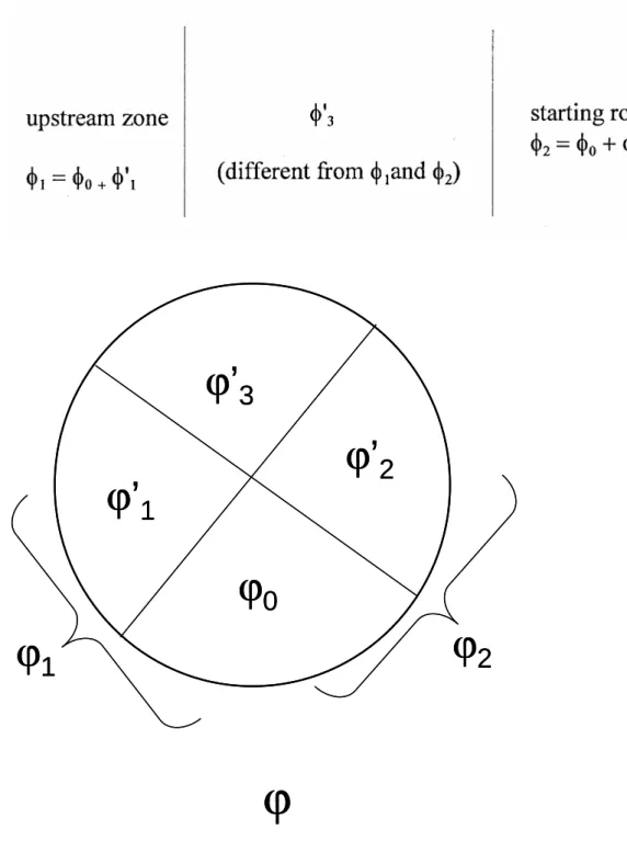
Let ϕ1 be the number of phases in the most external upstream zone (last zone) and ϕ2 be the number of phases in the starting rock (downstream
medium, first zone). Let ϕ0 be the number of phases common to ϕ1 and ϕ2; let us write ϕ1 = ϕ0 + ϕ'1 and ϕ2 = ϕ0 + ϕ'2. And let ϕ'3 be the number of phases that appear neither in ϕ1 nor in ϕ2; these phases appear in one zone then disappear in another. We then have
ϕ ≥ ϕ0 + ϕ'1 + ϕ'2 + ϕ'3 (7)
The value of total ϕ as given by (7) is a minimum because some phases must be counted several times if they are present in several zones. It does not seem useful to make a distinction between the phases that appear or disappear in the course of a precipitation or dissolution process rather than a chemical reaction with other phases: a reaction may be considered as the simultaneous
dissolution of a mineral and the precipitation of another. Let us compute z. A zone may appear because of: a) the appearing of a phase that was not in the starting rock; b) the disappearing of a phase with no appearing of any new phase; c) the replacement of a former phase by a new one, which we do not count as equivalent to a) + b).
Let us call ϕ'0 the number of phases that are merely replaced by c) mechanism. ϕ'0 is already counted among the preceding phases but it is interesting to consider it apart for the numbering of zones. We have in effect:
z ≤ 1 + (ϕ'1 + ϕ'3) + (ϕ'2 + ϕ'3) - ϕ'0 (8)
where 1 stands for the starting rock, (ϕ'1 + ϕ'3) stands for a) mechanism, (ϕ'2 +
ϕ'3) stands for b) mechanism and ϕ'0 stands for c) mechanism. ϕ'0 is subtracted because at each time such a replacement event occurs, it is necessary to count only one zone change and not two (as induced by ϕ'1 + ϕ'2). Relations (7) and (8) lead to:
z - ϕ ≤ 1 + ϕ'3 - ϕ0 - ϕ'0 (9)
and according to equation (2)
v ≤ (c - ϕ0) - ϕ'0 + ϕ'3 = (c - ϕ0) - (ϕ'0 - ϕ'3) (10)
which is equivalent to:
v ≤ c - (ϕ0 + ϕ'0) + ϕ'3 (10')
2. Interpretation of (10)
(c - ϕ0) is simply what is usually called c after some simplification: phases of ϕ0 type are those unchanged in the system, such as water or the minerals not involved in the chemical reactions, zircon, apatite and so on. ϕ'0 is
the number of minerals that undergo a replacement transformation of type c), for instance ϕ'2 →ϕ'1 and this does not modify the variance as has been said in section 5.2. These minerals are added to ϕ0 in (10'): in a way, they remain but modified for instance sphene → rutile in the albitites (Pascal, 1979). However, among these minerals, some are going to disappear, these are the minerals of
ϕ'3 type; ϕ'3 thus is a correcting of ϕ'0.
In brief, (ϕ'0 - ϕ'3) is a correcting of ϕ0 for the phases that persist while changing, where the change does not bring any modification in the number of associated phases. Phases ϕ'3 that appear then disappear in the system are subtracted, so that the phases that change from the start are counted but once.
3. Comparison with the intuitive variance
One could have thought the variance to be:
v ≤ v* = 2c - ϕ1 - ϕ2 (11)
v* corresponds to the sum of the maximum numbers of degree of freedom on the starting rock and on the inlet fluid sides. This may also be written:
v* = 2c - ϕ1 - ϕ2 = 2c - 2ϕ0 - ϕ'1 - ϕ'2 = (c - ϕ0) + (c - ϕ) + ϕ'3
= (c - ϕ0) - (ϕ - c) + ϕ'3 (12)
that we compare to (10). The quantity (ϕ - c) would be equal to ϕ'0 if all the transformations where of c) type. Generally, this is not the case, and the intuitive expression of the variance that leads to (12) must not be retained.
4. Another interpretation of v in (10)
The quantity ϕ'0 - ϕ'3 is the number of minerals in the rock equilibrated with inlet fluid that result from the transformation of minerals of starting rock.
In the Korzhinskii language, this is the number of determinant components that remain inert at the source. So v = c - ϕ0 - (ϕ'0 - ϕ'3) is the number of
components that remain inert at the source of the fluid, after subtracting the precipitated minerals, but including the accessories and the excess minerals.
Captions for figures
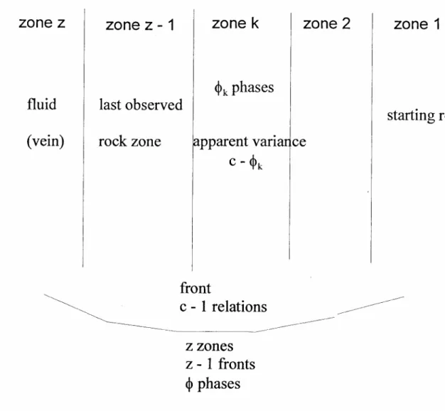
Fig. 1: The "connected" system of metasomatic zones. In zone number k, there
are ϕk phases and the apparent chemical variance is c - ϕk, where c is the number of chemical components. But the total variance is not Σz(c - ϕk) for all the z zones, because the z zones are not independent from a chemical point of view. This is due to the relations connecting the variations of the
concentrations in the fluid and in the solid at each reaction front. The overall variance of this connected system is given by v = c + z - ϕ - 1 where ϕ is the total number of phases, each counted the number of times as zones where present (see text).
Fig. 2: Categories of phases and of fronts; the total number of phases, ϕ, is divided into several groups; ϕ2 is the number of phases belonging to the starting rock; ϕ1 is the number of phases in the last solid zone. Among the ϕ2 phases, ϕ0 phases are common with that found in the last solid zone. ϕ'2 and ϕ'1 are such that ϕ1 = ϕ0 + ϕ'1 and ϕ2 = ϕ0 + ϕ'2. Inside the system of zones, ϕ'3 is the number of phases that are different from ϕ1 and ϕ2. These different phases allow the definition of several types of fronts. The generalized rule sets constraints on the different types of fronts depending on the values of ϕ0, ϕ1,
Fig. 1: The "connected" system of metasomatic zones. In zone number k, there are ϕk phases
and the apparent chemical variance is c - ϕk, where c is the number of chemical components.
But the total variance is not Σz(c - ϕk) for all the z zones, because the z zones are not
independent from a chemical point of view. This is due to the relations connecting the variations of the concentrations in the fluid and in the solid at each reaction front. The overall variance of this connected system is given by v = c + z - ϕ - 1 where ϕ is the total number of phases, each counted the number of times as zones where present (see text).
ϕ
’
1
ϕ
’
3
ϕ
0
ϕ
’
2
ϕ
2
ϕ
1
ϕ
ϕ
’
1
ϕ
’
3
ϕ
0
ϕ
’
2
ϕ
2
ϕ
1
ϕ
Fig. 2: Categories of phases and of fronts; the total number of phases, ϕ, is divided into several groups; ϕ2 is the number of phases belonging to the starting rock; ϕ1 is the number of phases in
the last solid zone. Among the ϕ2 phases, ϕ0 phases are common with that found in the last
solid zone. ϕ'2 and ϕ'1 are such that ϕ1 = ϕ0 + ϕ'1 and ϕ2 = ϕ0 + ϕ'2. Inside the system of zones,
ϕ'3 is the number of phases that are different from ϕ1 and ϕ2. These different phases allow the
definition of several types of fronts. The generalized rule sets constraints on the different types of fronts depending on the values of ϕ0, ϕ1, ϕ2, ϕ'1, ϕ'2 and ϕ'3 (see text).