HAL Id: hal-00679034
https://hal.archives-ouvertes.fr/hal-00679034
Submitted on 14 Mar 2012HAL is a multi-disciplinary open access archive for the deposit and dissemination of sci-entific research documents, whether they are pub-lished or not. The documents may come from teaching and research institutions in France or abroad, or from public or private research centers.
L’archive ouverte pluridisciplinaire HAL, est destinée au dépôt et à la diffusion de documents scientifiques de niveau recherche, publiés ou non, émanant des établissements d’enseignement et de recherche français ou étrangers, des laboratoires publics ou privés.
Clique separator decomposition in less than nm
Anne Berry, Romain Pogorelcnik
To cite this version:
Anne Berry, Romain Pogorelcnik. Clique separator decomposition in less than nm. 2010. �hal-00679034�
Clique separator decomposition in
less than nm
Anne Berry
1Romain Pogorelcnik
1Research Report LIMOS/RR-10-09 9 avril 2010
1
LIMOS UMR CNRS 6158, Ensemble Scientifique des C´ezeaux, F-63 173 Aubi`ere, France, [email protected], [email protected]
Abstract
We address the problem of computing the atoms of the decomposition by clique minimal separators of a graph G (also called the maximal prime subgraphs) when a minimal trian-gulation H of G is given as part of the input. We present a new algorithmic technique based on the clique tree of H.
We introduce a new graph parameter, m0, which is the number of edges belonging to no
min-imal separator of H. We give an algorithm which runs in O(nm0) time, which improves the
current O(nm) time for this problem. Another version of our algorithm runs in O(n(n + t)) time, where t is the number of 2-pairs of H.
We show that our technique computes the atoms in O(n2
) time for several graph classes, including the graphs with bounded treewidth, which improves the current O(n3
) time for dense graphs by a factor of n.
Keywords: clique separator decomposition, minimal triangulation, atom, maximal prime subgraph, chordal graph, clique tree
1
Introduction
Clique separator decomposition is a graph decomposition which uses the separators (or cutsets) inducing complete subgraphs.
The process was introduced by Tarjan [25] as a useful divide-and-conquer approach to solve hard problems such as maximum clique and coloring. He used a LEX M ordering of the graph to provide an O(nm) time implementation.
LEX M is an O(nm) time search designed for minimal triangulation computing [24]. Given a graph G = (V, E) (where |V | = n and |E| = m), a minimal triangulation is a chordal supergraph H = (V, E + F ) of G, such that if any of the added edges is removed, the graph is no longer chordal (a chordless 4-cycle has been created). F is called the fill, |F | = f , and the edges of F are called fill edges.
Tarjan’s algorithm was modified by [17] to use only clique separators which are also minimal separators, obtaining a canonical decomposition. The subgraphs obtained, called “atoms” [25] (or “maximal prime subgraphs” [17]) are defined as the inclusion-maximal connected subgraphs containing no clique separator. (The reader is referred to [3] for full details).
Recently, this decomposition has generated interest in several fields. It has been applied to Bayesian networks [21], to treewidth [7], to graph problems [8], to graph modelization of data from biochips [13] and from text mining [9].
As mentioned above, the only known way of finding the clique minimal separators effi-ciently is to use a minimal triangulation, by virtue of the following property :
Property 1.1 [2], [3], [22] Let G = (V, E) be a connected graph, let H = (V, E + F ) be a minimal triangulation of G. Then any clique minimal separator of G is a minimal separator of H.
The edges missing from the separators of H which are not cliques in G are precisely the edges of F , so each fill edge lies inside a minimal separator of H.
Computing the (less than n) minimal separators of a chordal graph can be done in linear time ([4], [6], [16]), so deciding which are cliques of the input graph can be done in O(nm) time by searching G(Si) for each separator Si.
When previous work was done on this decomposition, minimal triangulation cost O(nm) time [24], so no effort was invested into computing the atoms faster. In fact, the algorithm from [25] requires a separate graph search for each atom, which costs O(nm) time, as there may be n − 1 atoms. As a result, each of the three steps from this process (compute a minimal triangulation, check the minimal separators for completion, compute the atoms) requires O(n) graph searches, and thus O(nm) time.
However, minimal triangulation has given rise to many recent results, showing that this O(nm) time bound can be improved. On special graph classes, the cost of computing a minimal triangulation may be lower than O(nm) ; for example, [18] presents linear time algorithms for AT-tree claw-free graphs and for co-comparability graphs. In the general
case for non-sparse graphs, the O(n3
) time bound has been recently lowered : [16] offer an O(n2.69
) time bound, later improved by [12] to O(nαlogn) = o(n2.376
), where nα is the time
required to do matrix multiplication, currently n2.376.
Our purpose in this paper is to provide an approach to compute the atoms efficiently when a minimal triangulation H is given as part of the input. To accomplish this, we will use a clique tree of H (a clique tree is a compact representation of a chordal graph H, where the nodes are the maximal cliques of H, and each edge (Ki, Kj) represents a minimal separator
Ki∩ Kj of H. As will become clear later, the clique tree will avoid the costly systematic
graph searches.
Our approach, which will be detailed further on, is the following : given a graph G and a minimal triangulation H of G :
1. Compute the clique tree T of H.
2. Run through the edges of T and determine which ones correspond to a non-clique minimal separator of G.
3. Run through T and merge any two cliques Ki and Kj which are extremities of an edge
corresponding to a non-clique minimal separator of G.
In the tree T′ obtained in the end, which we call the atom tree, the nodes are the atoms
of G and the edges are the clique minimal separators of G.
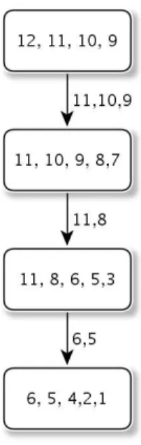
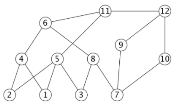
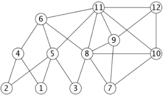
Example 1.2 Figure 1 gives graph G, and Figure 2 gives a minimal triangulation H of
G, with the fill edges represented by dashed lines. Figure 3 gives the clique tree of H ; the minimal separators of H which are not cliques of G are : {10, 9, 8}, {8, 5} and {5, 4}. Figure 4 gives the atom tree T′ obtained in the end.
Fig. 1 – A non-chordal graph G.
Step 1 can be done in O(m + f ) time, using the algorithm from [6]. Step 3 can easily be done in O(n2
), as merging two cliques costs O(n), and there are less than n edges in a clique tree. This clique merging process, presented in [21], is of primary importance : it enables us to compute the atoms without requiring an O(m) time graph search each time a clique minimal separator of G is detected. In fact, T′ is a clique tree of
Fig.2 – Chordal graph H, a minimal triangulation of graph G from Figure 1, with an MCS numbering. The minimal separator generators are marked by a star.
Fig. 3 – The clique tree T of graph H from Figure 2, generated by the algorithm from [6]. The label of each node is framed. The minimal separator generators are marked by a star.
a clique. G∗ was devised to be a chordal graph which has the same atoms and the same
clique minimal separators as G.
Our complexity bottleneck thus resides in Step 2, i.e. in deciding which separators of the minimal triangulation H are cliques of the input graph G. As mentioned above, this is easily done in O(nm) time, but our aim is to propose techniques to accomplish a better time.
There are cases when Step 2 can be done efficiently in a straightforward fashion : 1. When the fill is of small size, each fill edge ab of F can be tested to see which minimal
Fig. 4 – The atom tree T′ of graph G from Figure 1, computed from clique tree T from
Figure 3.
costs nf time, which may be lower than nm when the fill is small. This approach is interesting in the context of triangulations computed with the Minimum Degree Heuristic, which approximates minimum triangulation and often yields a very small fill in practice ; recent research has shown how to extract a minimal triangulation in O(f (m + f )) time [5].
2. A minimal separator S = {s1, s2, ..., sk} of H can be tested for completeness by testing
for the presence in G of each edge sisj of S. All the clique minimal separators of G
can thus be found in time proportional to the sum of the number of edges over all the minimal separators of H. As these separators may overlap, in the worse case this approach costs O(nm) time. However, this number may be small, and can be evaluated as the minimal separators of H are computed.
In view of improving the cases where none of the above present a gain over the O(nm) time complexity, we present an algorithmic process which traverses the clique tree, testing each edge for completion.
Our technique, which will be detailed in Section 3, represents each separator S by a “super-vertex”, which is the contraction of all the vertices of S. We modify this super-vertex while running through T by adding or removing vertices as we go along, so that the current minimal separator is represented by the current super-vertex. This technique presents a gain because instead of checking each edge inside each separator of H, we just check one super-vertex for being adjacent to a fill edge. Thus, when separator S is detected as being non-complete, we do not know exactly which edges of S are fill edges, but we do not need this information. Our complexity will reside in the number of additions or removals of vertices, and we will see that this number may be small.
– When T is traversed from top to bottom, we obtain a complexity of O(n(n+t)), where t is the number of 2-pairs of H, which is in O(n(m − f )), where m is the number of edges of complement G of G.
– When T is recursively traversed from bottom to top, we obtain a complexity of O(nm0), where m0 is the number of edges of H which belong to no minimal
sepa-rator of H. m0 is at most m and can be considerably smaller.
Thus our new approach can do no worse than the classical one, and offers a possibility to obtain a much better time. We will see in our discussions in Section 3 that there are many cases where our complexity is in O(n2
), thus offering a gain of a factor of n for dense graphs, which are precisely the graphs for which the cost of triangulation has been recently improved upon in the general case.
The paper is organized as follows : after this introduction, we give few preliminaries in Section 2, then present in detail our new technique in Section 3, before concluding.
2
Preliminaries
The graphs in this paper are finite, undirected and connected. For a graph G = (V, E), V is the set of vertices, |V | = n and E is the set of edges, |E| = m. For any subset X of V, G(X) denotes the subgraph of G induced by X (for the sake of simplicity, we will often not distinguish between a vertex set and the subgraph it induces). For a graph H, we will sometimes denote by E(H) the vertex set of H. For any vertex v of G, NG(v) denotes the
neighborhood of v in G. A set of vertices X is complete or a clique if its vertices are pairwise adjacent.
Separation. In a connected graph G = (V, E), a subset S of V is a separator of G if G(V −S) is disconnected. For any non-adjacent vertices a and b, S is an ab-separator if a and b are in different connected components of G(V − S). S is called a minimal ab-separator if it is an inclusion-minimal ab-separator, and a minimal separator if there is some pair {a, b} such that S is a minimal ab-separator. A 2-pair is a pair {a, b} of non-adjacent vertices such that every path from a to b is of length exactly 2 [11]. In a connected graph, {a, b} is a 2-pair iff N (a) ∩ N (b) is a minimal separator [1], [15].
Chordal graphs. A graph is chordal, or triangulated, if it contains no chordless cycle of length ≥ 4. A connected graph is chordal if and only if all its minimal separators are cliques [10]. A chordal graph has less than n minimal separators and less than n maximal cliques [23]. A chordal graph H = (V, E + F ) is called a triangulation of non-chordal graph G= (V, E). The set F of edges, of size |F | = f , is called a fill. A triangulation H is minimal if ∀e ∈ F , (V, E + F − {e}) is not chordal [24]. MCS [26] numbers the vertices of a chordal graph from n to 1. In the numbering π of V obtained, π(x) will denote the number of vertex x, and the upper neighborhood of x is M adj(x) = {y 6= x|π(y) > π(x)}. A vertex x is called a minimal separator generator (or a generator for short) if M adj(x) is a minimal separator and |M adj(x)| ≤ |M adj(y)|, where π(y) = π(x) + 1 [4].
3
Using the clique tree to find the clique minimal
se-parators
We will now explain our new process in detail. We will first consider the properties of the clique tree we construct, then explain our processes for running through the tree, and give a detailed complexity analysis for each. We will the compare the merits of the two approaches, in the general case as well as for some special graph classes.
3.1
Building the clique tree
We will use the clique tree T induced by an MCS execution of the given minimal trian-gulation H, as detailed in [6]. This costs O(m + f ) time. As is the case for any clique tree, for each vertex x of H, the nodes of T containing x define a subtree. We will label each node with the vertex (or vertices) for which it is the root of the corresponding subtree. Each node Ki of T thus bears as label a different vertex (or set of vertices). The vertices of a label
bear consecutive numbers. Each of the these labels contain exactly one minimal separator generator, which is its vertex of largest number, call it x ; M adj(x) is exactly equal to the minimal separator stemming up from Ki.
When the algorithm from [6] for constructing the clique tree is used, the labels define a heap structure : for each subtree with root Ki, the label of Ki contains vertices whose
numbers are larger than that of any of the vertices of the other labels of the subtree.
Example 3.1 Figure 2 shows a chordal graph H whose vertices are numbered by an execu-tion of MCS. The minimal separator generators are marked by a star. Figure 3 shows the corresponding clique tree with its labels (which are framed), organized into a heap. Clique
{11, 8, 6, 5} has label {6, 5}. The vertex of highest number of {6, 5} is 6, a minimal
separa-tor generasepara-tor. M adj(6) = {11, 8}, which is the minimal separasepara-tor stemming up from clique
{11, 8, 6, 5}.
As mentioned above, we will search T in two different ways : by a Top-to-bottom and by a recursive Bottom-to-top approach, with a different complexity analysis for each.
Our technique in both cases is the same. In order to test a separator S for completeness, we will represent S in a global fashion by a super-vertex of G(F ), which is the contraction of all the vertices of S (the neighbors of this super-vertex will be the union of all the neighborhoods of the vertices of S).
Our algorithms start with a super-vertex representing either the root or a leaf of T , and moves this super-vertex through T , modifying it by adding or removing vertices of V in order to represent the current minimal separator.
Addition and removal of nodes to a super-vertex X are defined as follows, using as base the matrix M of G(F ) :
– Removing vertex x from X : for each y such that xy ∈ F , decrease (y, X) by one. Note that the multiplicity of each edge of X is stored in the corresponding entry of the modified matrix of G(F ).
Each addition or removal of one vertex costs n time. To compute the super-vertices of an initial clique Ki, start with any vertex v of Ki, and add the other vertices one by one
using the process above.
A minimal separator S = {s1, s2, ..., sk} represented by super-vertex X is tested for
completeness by simply checking whether all siX entries the matrix of G(F ) are null. If
they are, then S is memorized as a clique minimal separator of G. If at least one value is non-zero, then S is memorized as a non-clique separator.
We will now describe and analyze the complexity for the two approaches.
3.2
The Top-to-bottom approach
For a Top-to-bottom approach, we initialize as super-vertex the root of T (which contains the vertex numbered as n by MCS), and then move through T in a Breadth-First fashion, each separator’s super-vertex being computed from that of its father in T .
Example 3.2 On the clique tree of Figure 3, a super-vertex representing vertex set {12, 11, 10, 9} is created as initialization, then 12 is removed to create minimal separator {11, 10, 9}, which is tested for completeness, and so forth.
Complexity of the Top-to-bottom approach.
Initialization : Initializing the root clique K costs (n − 1).|K|, which is in O(n2
).
Vertex additions : Each vertex x of V will be added at most once, when the root of the
subtree of x is reached, so the global cost is less than n2
. (Note that some vertices are never added, for instance the ones labeling the cliques which are leaves of T ).
Vertex removals : Consider vertex x being removed from clique Ki to describe the
mi-nimal separator Ki∩ Kj between Ki and the child clique Kj of Ki. Let y be the generator
from the label of Kj. Because of the heap structure of T , y does not appear higher than Kj
in T , so y is not adjacent to x. x and y are at distance 2 in H, since for any s ∈ Ki∩ Kj,
s is adjacent to both x and y, so there is a chordless path (x, s, y) in H. It is easy to see that NH(x) ∩ NH(y) = Ki ∩ Kj = M adj(y) = S. Thus {x, y} form a 2-pair. Each vertex
removal is associated with a unique 2-pair {x, y} such that π(x) > π(y) and y is a minimal separator generator.
Example 3.3 On the clique tree of Figure 3, vertex 8 is removed when moving from clique
{11, 8, 6, 5} to clique {6, 5, 4} ; this removal is associated with the 2-pair {8, 4} ; NH(8) ∪
NH(4) = {6, 5}. 8 and 4 are at distance 2 in H.
It is easy to compute the exact number of vertex removals in O(n2
) by traversing T and computing, for each edge (Ki, Kj), Ki− (Ki∩ Kj).
This number of vertex removals is bounded by the number t of 2-pairs of H, which is bounded by |E(H2
)|−|E(H)|, with |E(H)| = m+f , so by |E(H2
)|−m−f . |E(H2
)|−|E(H)| is in turn bounded by |E(H)|, which is m − f .
Thus the Top-to-bottom approach runs in time O(n(n + t)), which is in O(n(|E(H2
)| − m− f )), which in turn is in O(n(m − f )).
3.3
The recursive approach
Our second approach is recursive. The initial call is on the root node of T . Each node Ki is recursively processed as follows :
– If Kiis a leaf, then create the super-vertex corresponding to the separator Si stemming
up towards the father clique, and test Si for completion.
– If Ki is not a leaf, then procure (by a recursive call on each child) the super-vertices
of the minimal separators stemming towards the children of Ki. Take any one, and
compare it with a second one, add any missing vertices to create a larger super-vertex, and so on, until all the children of Ki in T have been merged into a new
super-vertex, add any vertices which are in Ki but in none of Ki’s children. A super-vertex
representing Ki is obtained. Modify Ki so that it represents the separator Si between
Ki and the father of Ki, and test S for completeness.
Example 3.4 On the clique tree of Figure 3, processing the clique labeled {6, 5} will require adding 6 to child super-vertex {8, 5}, since {8, 5} − {6, 5} = {6}. Vertex 11 is then added to obtain the entire clique {11, 8, 6, 5}. Minimal separator {11, 8} is then obtained from clique
{11, 8, 6, 5} by removing vertices 6 and 5.
In order to accomplish our complexity analysis, we will define the graph parameter m0
which we introduce :
Definition 3.5 Let G = (V, E) be a graph, let H = (V, E + F ) be a minimal triangulation of G. We define the desaturated graph of H, denoted by H0, as the graph obtained from H
by removing all the edges which have both endpoints inside some common minimal separator
S of H. We denote by m0 the number of edges of H0.
H0 can easily be computed in nα time using the square of the bipartite graph between
the minimal separators and the vertices.
Example 3.6 Figure 5 gives the desaturated graph H0 of chordal graph H from Figure 2.
Each edge of H0is also an edge of G, as any minimal triangulation is obtained by making
some minimal separators of G into cliques which will be the minimal separators of H [22], [2]. Thus m0 6m. When the minimal separators of H are large, m0can be much smaller than m.
Fig. 5 – The desaturated graph H0 of H.
Initialization : Let S = {s1, s2, ..., sk} be a separator stemming up from a leaf K of T ,
and let x be a vertex from the label of T . All the pairs xsi, si ∈ S, belong to E(H), since
they are together in clique K, but they belong to no minimal separator, since no other clique can contain both x and si, because of the heap structure of T . Thus each addition step of
a vertex si during the initialization is associated with a unique edge xsi of H0.
Vertex removals : Each vertex x is removed at most once, when the root of the subtree
of x is reached, thus the vertex removals cost O(n2
) globally.
Vertex additions : A vertex addition step is necessary when vertex x appears in clique
Ki but appears in none of the child cliques of Ki. We can also bound the number of vertex
additions using m0 : let y be a vertex from the label of Ki : xy is an edge of H (since x and
y are together in clique Ki), but xy belongs to no minimal separator, since x and y can be
in no other clique together.
Globally, the recursive approach thus requires O(nm0) time.
Note that, aside from the initialization step, the vertex addition steps in the recursive approach form a subset of the vertex removal steps in the Top-to-bottom approach. Thus it is not necessary to compute m0 to decide if this approach is better than the other one : the
cost of the initialization is the prevailing factor, which can be evaluated in O(n).
Example 3.7 In our example from Figure 3, in the recursive approach, 11 is added to form clique {11, 8, 6, 5} from its children {8, 5, 3} and {6, 5, 4} ; this corresponds to 2 vertex removals in the Top-to-bottom approach. 8, on the other hand, need not be added at this step by the recursive approach, since 8 already appears in child clique {8, 5, 3}.
3.4
The merits of the Top-to-bottom approach versus the
recur-sive approach
As mentioned in our complexity analysis, aside from the initialization step, the recursive approach does only a subset of the steps required by the Top-to-bottom approach. Therefore, the only drawback of the recursive approach is the initialization step. This is costly only when the minimal separators which correspond to the leaves of T present a large vertex overlap. This overlap is easily tested when building the clique tree.
In any case, m0 is at most m, and may be much smaller, so using the recursive approach
cannot be worse than using the classical method.
When initializing the leaves is costly, however, or when m0 is of order m, the
Top-to-bottom approach may be very interesting. This is the case when the number of 2-pairs of H is small. It is also interesting that with this approach, the final tree T′can be computed with
a single pass of MCS ; as a result, the Top-to-bottom approach uses only local information, and may be useful for handling very large graphs.
As discussed previously, the exact cost of each approach can be forecast in O(n2
) while building the clique tree, so the user can choose the best approach at no extra cost.
Let us finish this section by discussing some special cases.
– When input graph G is of bounded treewidth, the size of the maximal cliques of H, and thus also the sizes of the minimal separators, are bounded. In the recursive approach, the initialization will cost O(n2
). The number of vertex additions is at most k per clique, so will cost O(kn) per clique, so overall the vertex additions will cost. When Gis f bounded treewidth, the recursive approach will thus run in O(n2
). – Applied to AT-free graphs, both our approaches will cost O(n2
), since the minimal triangulation is an interval graph [20] and thus the clique tree is a path : each vertex will be added and removed at most once.
– For graphs where m is small, [19] recently proposed a minimal triangulation algorithm in O(m(δ2
+m)), where δ is the maximum degree of G, so the Top-to-bottom approach nicely complements this work.
– When the number of leaves of T is bounded by k, the Top-to-bottom approach will run in O(n2
), as for a given vertex x, the number of vertex removals is less than k, so each vertex will cost O(kn).
We conjecture that there are many other graph classes where our algorithms will offer an O(n2
) time.
4
Conclusion
We present a new technique to compute the atoms of the clique minimal separator decomposition of a graph when a minimal triangulation is given as input, using a clique tree.
Contrary to the classical methods, our approach does not require graph searches, but the clique tree is searched instead, which is much more efficient.
We introduce a new graph parameter, m0, which is less than m, which we use to bound
in nm0 time our recursive approach.
Our Top-to-bottom approach is in O(n(n + t)), where t is the number of 2-pairs of H. In many cases, our algorithms run in O(n2
) time, thus improving by a factor of n for dense graphs the pre-existing O(nm) time method for computing the atoms.
Acknowledgement
The authors thank Christian Laforest for his valuable suggestions for this paper.
R´
ef´
erences
[1] S. R. Arikati and C. P. Rangan. An efficient algorithm for finding a two-pair, and its applications. Discrete Applied Mathematics, 31 :1 (1991) 71-74.
[2] A. Berry, J.-P. Bordat, P. Heggernes, G. Simonet and Y. Villanger. A wide-range algorithm for minimal triangulation from an arbitrary ordering. Journal of Algorithms, 58 :1 (2006) 33-66.
[3] A. Berry, G. Simonet and R. Pogorelcnik. An introduction to clique minimal separator decomposition. Research Report LIMOS RR-10-03 (2010).
[4] A. Berry and R. Pogorelcnik. A simple algorithm to generate the minimal separators of a chordal graph. Research Report LIMOS RR-10-04 (2010).
[5] J. R. S. Blair, P. Heggernes and J. A. Telle. A practical algorithm for making filled graphs minimal. Theorical Computer Science, 250 :(1-2) (2001) 125-141.
[6] J. R. S. Blair and B. W. Peyton. An introduction to chordal graphs and clique trees.
Graph Theory and Sparse Matrix Computation, 84(1-3) (1993) 1-29.
[7] H.L. Bodlaender and A.M.C.A. Koster. Safe separators for treewidth. Discrete
Mathe-matics, 306 (2006) 337-350.
[8] A. Brandst¨adt and C.T. Ho`ang. On clique separators, nearly chordal graphs, and the Maximum Weight Stable Set Problem Theoretical Computer Science 389 (2007) 295-306.
[9] M. Didi Biha, B. Kaba, M.-J. Meurs, E. SanJuan. Graph Decomposition Approaches for Terminology Graphs. MICAI (2007) 883-893.
[10] G. A. Dirac. On rigid circuit graphs. Abh. Math. Sem. Univ. Hamburg, 25 (1961) 71-76. [11] R. Hayward, C. Hoang, and F. Maffray. Optimizing weakly triangulated graphs. Graphs
and Combinatorics, 5 (1989) 339-349.
[12] P. Heggernes, J. A. Telle, Y. Villanger. Computing Minimal Triangulations in Time O(nαlogn) = o(n2.376
). SIAM Journal on Discrete Mathematics, 19 :4 (2005) 900-913. [13] B. Kaba, N. Pinet, G. Lelandais, A. Sigayret, A. Berry. Clustering gene expression
data using graph separators. In Silico Biology, 7 :(4-5) (2007) 433-452.
[14] D. Kratsch, J. Spinrad. Minimal fill in O(n2.69) time. Discrete Mathematics, 306 :3
(2006) 366-371.
[15] J. Spinrad and R. Sritharan. Algorithms for weakly triangulated graphs. Discrete
Applied Mathematics, 59 (1995) 181-191.
[16] P. Sreenivasa Kumar and C. E. Veni Madhavan. Minimal vertex separators of chordal graphs. Discrete Applied Mathematics, 89(1-3) (1998) 155-168.
[17] H.-G. Leimer. Optimal decomposition by clique separators. Discrete Mathematics, 113 (1993) 99-123.
[18] D. Meister. Recognition and computation of minimal triangulations for AT-free claw-free and co-comparability graphs. Discrete Applied Mathematics, 146 :3 (2005) 193-218. [19] M. Mezzini and M. Moscarini. Simple algorithms for minimal triangulation of a graph and backward selection of a decomposable markov network. Theoretical Computer
Science, 411 :(7-9) (2010) 958-966.
[20] R. H. Moehring. Triangulating graphs without asteroidal triples. Discrete Applied
Mathematics, 64 (1996) 281-287.
[21] K.G. Olesen and A.L. Madsen. Maximal prime subgraph decomposition of Bayesian networks. IEEE Transactions on Systems, Man and Cybernetics, Part B : Cybernetics 32 :1 (2002) 21-31.
[22] A. Parra and P. Scheffler. Characterizations and Algorithmic Applications of Chordal Graph Embeddings. Discrete Applied Mathematics 79 :(1-3) (1997) 171-188.
[23] D. J. Rose. Triangulated graphs and the elimination process. Journal of Mathematical
Analysis and Applications, 32 :3 (1970) 597-609.
[24] D. J. Rose, R. E. Tarjan, and G. S. Lueker. Algorithmic aspects of vertex elimination on graphs. SIAM Journal on Computing, 5 (1976) 266-283.
[25] R.E. Tarjan. Decomposition by clique separators. Discrete Mathematics, 55 (1985) 221-232.
[26] R. E. Tarjan and M. Yannakakis. Simple linear-time algorithms to test chordality of graphs, test acyclicity of hypergraphs, and selectively reduce acyclic hypergraphs.
![Fig. 3 – The clique tree T of graph H from Figure 2, generated by the algorithm from [6].](https://thumb-eu.123doks.com/thumbv2/123doknet/14576884.540333/6.892.296.607.414.783/fig-clique-tree-t-graph-figure-generated-algorithm.webp)