HAL Id: hal-02091263
https://hal.uca.fr/hal-02091263
Submitted on 5 Apr 2019
HAL is a multi-disciplinary open access
archive for the deposit and dissemination of
sci-entific research documents, whether they are
pub-lished or not. The documents may come from
teaching and research institutions in France or
abroad, or from public or private research centers.
L’archive ouverte pluridisciplinaire HAL, est
destinée au dépôt et à la diffusion de documents
scientifiques de niveau recherche, publiés ou non,
émanant des établissements d’enseignement et de
recherche français ou étrangers, des laboratoires
publics ou privés.
Elementary Algorithms for Multiresolution Geometric
Tomography with Strip Model of Projections
Yan Gérard
To cite this version:
Yan Gérard. Elementary Algorithms for Multiresolution Geometric Tomography with Strip Model of
Projections. 2013 8th International Symposium on Image and Signal Processing and Analysis (ISPA),
Sep 2013, Trieste, Italy. pp.600-605, �10.1109/ISPA.2013.6703810�. �hal-02091263�
Elementary Algorithms for Multiresolution
Geometric Tomography with Strip Model of
Projections
Yan Gerard
ISIT - UMR 6284 CNRS / Universit´e d’Auvergne Clermont-Ferrand - France
Email: [email protected]
Abstract—We consider a problem of geometric tomography whith a strip-based model of projections: the projections are the areas of the intersection between the shape and some strips. We investigate some elementary algorithms that allow to construct a shape with prescribed projections. We start with an exact algorithm based on Linear Programming which leads to practical difficulties. Then we investigate three practical heuristics based on a cell decomposition of the domain of interest: GA is a greedy algorithm, GAME its multiresolution derivative and MPH a multiresolution heuristic close to a parallel Simulated Annealing.
According to Richard Gardner, Geometric tomography deals with the retrieval of information about a geometric object from data concerning its projections (shadows) on planes or cross-sections by planes. [1]. The main class of problems of this field is to provide some algorithms of reconstruction of an unknown compact shape S from projections in some directions. Several kind of projections can be considered but the most classical way is to consider X-rays that cross S and provide an information about its length or cardinality along each beam. We will focus our attention on the reconstruction of sets from projections with a finite set of directions and a finite number of sensors.
I. PROBLEMSTATEMENT
A. Back to Radon Transform
We place us in a 2D framework and denote Dθ,r the line
of equation xcosθ + ysinθ = r. We consider a compact shape S and its characteristic function fS : R2 → {0, 1}.
With this basic formalism, the X-ray of S in the direction θ ∈ [0, π[ is the function XθS : R → R defined by
XθS(r) =RD
θ,rfS(x(s), y(s))ds where s denotes the abscissa
along the curve. Generally speaking, the function XθS(r) of the two variables θ and r is known as the Radon transform of f and its 2D image is called the sinogram of f .
The inverse problem of computation of f from its sinogram has been introduced in 1917 [2]. It can be solved with Fourier analysis by using the Fourier Slice theorem [3]: This solution works also with binary functions as the characteristic function fS and thus allows to reconstruct an unknown shape from its
Radon transform.
B. Why is the problem still interesting?
Hundred years after, there exists more than 20 types of tomography, from microtomography to Positron Emission
Tomography, but whatever the goal and the physical process involved in these systems, there is a major difference with previous Radon model: the measurements are always discrete. The number of directions of the X-rays can go from 2 to several hundreds -it is finite- while the number of sensors is also bounded. These numbers will increase with the technology improvement but there will still remain some cases where the number of directions will remain very small because the measurements can degrade the object while in the framework of medical imaging, it is always better to reduce the radiation doses. It is a reason to investigate deeply the reconstruction techniques which can deal with only a few projections.
It is well known since several years that in this framework -let’s say with 2, 3 until 15 directions- classical techniques of computerized tomography becomes inefficient. They fail especially in geometric tomography since they don’t take into account the a-priori that the image to reconstruct is binary. C. Length ray and strip-based Models
There are at least two different models for the X-rays of a shape S in a given direction. The classical one is the length ray model. For each beam, the X-ray measured ”behind” the shape provides the length of the intersection between the shape and the beam namely XS
θi(r
i
j) for the finite sequences of directions
θi and offsets rij (usually these sequences have a regular steps
∆θ and ∆r). This model is the one considered usually in
geometric tomography with a variant in the case of a cone beam.
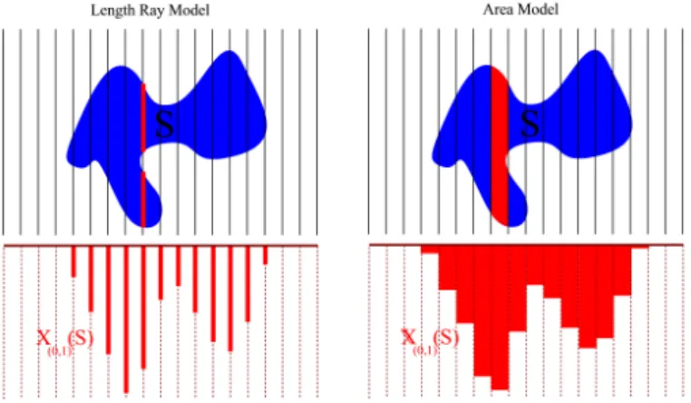
The second model comes from the idea that a sensor can not capture the energy coming from a single beam but the one of all the beams reaching its surface (Fig. 1). With a given direction θ, this set of beams makes a strip. This idea has been introduced in 1956 by R.N. Bracewell in his old paper ”Strip integration in radio astronomy” [3] and investigated more recently in the framework of discrete tomography [4], [5]. Let us denote Dθ,[rj,sj] the strip rj≤ xcosθ + ysinθ ≤ sj
where rj and sj are the extremal offsets of the sensor of
index j. It follows that in this model, with X-rays in direction θi, the value captured by this sensor is not XθSi(rj) but
its sum XS θi[j] =
Rsj
r=rjX
S
θi(r)dr namely the area of the
intersection between the strip Dθi,[rj,sj] and the unknown
shape S. To avoid confusion, these theoretical measurements XSθ[i] are called X-areas instead of X-rays in this paper. These
Fig. 1. Length Ray and Area models. On the left, in the length ray model, the projection is given by the length of the intersections between lines and S while in the area model, on the right, the projection is the area of the intersection of a strip and S.
continuous model where the function XθSi is perfectly known if the resolution of the ”camera” leads to infinite.
D. What’s the original problem?
We are interested in the reconstruction of an unknown shape S from its X-areas. The input of the problem is a two-dimensional finite sequence ai,j and a set of strips Dθi,[rij,sij]
with directions θiand offsets in the interval [rij, sij]. The output
is a set S verifying ∀i, j, XSθi[j] = ai,j if there exists one.
Notice that we don’t make any assumption on S while it is usual in the framework of geometric tomography to consider almost convex shapes since otherwise, with the length ray model, the problem becomes trivial (any union of segments with prescribed lengths is a solution). With X-areas, no such trivial solutions exists. The aim of the paper is to investigate the most elementary ideas that could allow to solve it. We start in next section with an exact solution by using Linear Programming. We didn’t test this approach since as we will see, it remains some difficulties to overcome. Then we will investigate and make experiments with greedy algorithms and a probabilistic heuristic in a multiresolution framework.
II. LINEARPROGRAMMING
A. Linear Program Statement
We assume now that the shape to reconstruct belongs to a known compact domain as for instance [0, 1]2. We do not assume that it is an union of pixels, it can be any subset of [0, 1]2 since we remain here in a continuous framework. Let us now take a strip Dθi,[ri
j,sij] for each direction θi. Their
intersection is either empty, or a polytope P . The set of all these polytopes defines a ”partition” of [0, 1]2 (the polytopes
just overlap on their faces namely on sets of null area) (see Fig. 2).
If there exists a solution S to a given instance of our reconstruction problem, then the intersection of S with the polytope P has an area x which is at least 0 and at most equal to the area of P : 0 ≤ x ≤ area(P ). If this area is strictly in this interval, then many other solutions S0 can be derived
from S just by moving the points of S in P . It means that the distribution of the points of a solution in each polytope P is not constrained. The only constraint is on x.
Fig. 2. Partition of the domain of interest [0, 1]2 in polytopes. The 8 strips of width 18 in four directions 0, π3, π2, 2π3 define a partition of the domain in 220 polytopes.
It leads to introduce a variable of area xkfor each polytope
Pk of the partition associated with the geometry of the strips
(let us denote K the set of indices of all the polytopes of the partition of [0, 1]2)). Each variable xk is constrained by
the double inequality 0 ≤ xk ≤ area(Pk). The prescribed
value of the area of the intersection of S with the strip Dθi,[rji,sij]of index j in direction θiprovides the linear equality
P
k∈Ki,jxk = ai,j where Ki,j is the list of indices of the
polytopes included in Dθi,[rij,sij](they provide a partition of the
strip in the considered domain [0, 1]2). It leads to a problem
of feasibility of linear equalities and inequalities ∀i ∈ I, j ∈ J, X
k∈Ki,j
xk= ai,j
∀k ∈ K, 0 ≤ xk ≤ area(Pk).
where I and J are the set of indices for the directions and sensors. It’s a problem of Linear Programming that can be solved by many kind of algorithms of this field (Simplex, Interior points,...).
In practice, due to noise and imprecision of float arithmetic, the equalitiesP
k∈Ki,jxk = ai,j should be relaxed in linear
double-inequalities ai,j − δi,j ≤ Pk∈Ki,jxk ≤ ai,j + δi,j
where the new variable δi,j denotes the error on the X-area
in the strip Dθi,[rji,sij]. Then a good objective function is the
sum of the errorsP
i∈I,j∈Jδi,j. Its minimization guarantees to
find a solution with a minimal error sum and an exact solution exists if and only if this minimum is null.
B. How Many Variables Has the Linear Program?
We have one constraint by strip and two constraints by variable and we have one variable by polytope in the partition of the domain of interest [0, 1]2. But how many polytopes are there in the partition of the unit square? If we have only one direction, it is the number of strips, denoted by n. If we have two directions, it is n2. If we have three directions (0, π3, 2π3)
and an even number of strips, it is 3n22 while if the number of strips is odd, it becomes 3n22−1. If we increase now the number of directions further than 4, the computation of the number of polygons becomes tedious (Fig. 3).
Fig. 3. Patterns of the partition of the domain of interest [0, 1]2 in polytopes. We cut again it with respectively 8 (left), 16 (right) directions with 8 strips of width 0.125 which turn around the center of the square and count the number of polytopes inside. It appears symmetries. With 2 strips, we have 64 polytopes. With 4 directions with an angular step π4 (0, π4, π2, 3π4 ) , we count 29 × 8 = 232 polytopes. With 8 directions with an angular step π8, we count 50 × 16 = 800 polytopes. With 16 directions with an angular step16π, it starts to be hard to count the number of polytopes without computing.
Then, an interesting question is to provide a general for-mula for the number N (n, d) of polygons for n strips turning in d direction with an angular steps πd. Even the asymptotic behavior of this function would be interesting because it determines if Linear Programming is suitable in practice in our framework.
C. From areas to shapes?
Let us assume now that the values of the areas xk of S in
each polytope Pk have been obtained by any method of Linear
Programming. It remains to choose the position of the points of S in each polytope. There could be some strategies but it is not straightforward. A second difficulty is to find an efficient way to compute the geometry of all polytopes Pk when their
number becomes very large. These open questions lead us to investigate other approaches coming from image processing, discrete tomography and operational research.
III. MULTIRESOLUTION FRAMEWORK
A. The cell partition of the domain
From a practical point of view, the goal is not necessarily to compute an exact solution but a binary image which is as close as possible to be or represent a solution. For this purpose, we are going to investigate a multiresolution approach. A multiresolution process starting from a low resolution solution to go to a high resolution final result has been introduced in several papers of Computerized Tomography [6], [7], [8]. We will also adopt the principle to refine a current solution during the computation but the main idea of this work is to keep at any time a multiresolution decomposition of the domain [0, 1]2
with very small cells on the boundaries of S and large cells where it is possible. It leads to use in practice the classical multiresolution decomposition of an image in quad-trees [9]. Nevertheless, instead of describing the present work only on
quad-trees, we prefer to stay as general as possible and just keep the properties that we will use in the following. Then we choose to present the results with an elementary data structure which is just a partition of the unit square in cells Ck with an
index k ∈ K (the cells can just overlap on regions of null area). These cells can be the pixels of an image of the unit square with [0, 1]2 or the leaves of a quad-tree. In this framework, a shape S is a subset of cells of indices in KS. We can also
consider its characteristic function fS : K −→ {0, 1} telling
if the cell is in S (its value is 1 or its color is black) or outside (0 for white).
B. Error minimization
We consider now our problem of reconstruction of a unknown shape with a prescribed X-area ai,j in each strip
Dθi,[ri
j,sij]. It can be formulated as a problem of minimization,
minimization of the error sum of the projections of a current shape S towards the prescribed values ai,j:
Errora(S) =
X
i,j
|ai,j− XSθi[j]|.
An exact solution S has a null error sum. There exists of course a lot of possible approaches to tackle this kind of problem and we choose to restrict ourselves to the algorithms that take a current shape S and just change the colors of a small number of cells at each step. These approaches are local or continuous in the sense that, at each step, the new shape S is close to the previous one according to the Hausdorff distance. Then the question is to determine the cells Ck whose colors should
be modified. We introduce in this goal two values of energies that control our elementary heuristics.
C. Mean and Absolute Energy Fields
The question is to determine which cells of the image should change their color in order to decrease the error sum. Of course, the cell Ck is only involved in the errors on the
X-areas in the strips which cross it. We can also notice that given a strip Dθi,[ri
j,sij], a cell Ck has in all likelihood a larger
contribution to the error ai,j−XSθi[j] if its intersection with the
strip is large. This idea leads to weight the contribution of a cell Ckto the error term ai,j−XSθi[j] by the area of the intersection
between the cell and the strip namely area(Ck∩ Dθi,[rij,sij]).
Then we introduce two values that we call mean and absolute energyfields:
M Ea(Ck) =
X
i,j
area(Ck∩ Dθi,[rij,sij])(ai,j− X
S θi[j])
AEa(Ck) =
X
i,j
area(Ck∩ Dθi,[rji,sij])|ai,j− X
S θi[j]|.
Since the unit square has an area equal to 1, the sum of the absolute energy fields for all cells is the error sum:
X
k∈K
AEa(Ck) = Errora(S).
The absolute energy provides a way to evaluate a contribution of each cell to the error sum that we would like to minimize. The mean energy obtained by keeping the signs of each error allows to determine if there is a deficit or an excess of color
in a cell. It there is a lack of black in the strips around the cell Ck, it appears with a positive mean energy while a lack
of white appears with a negative value.
At last, we precise that our heuristics use energy densities instead of the intrinsic values: the mean and absolute energy densities of the cell Ckare respectively AED(Ck) = Area(CAE(Ck)
k)
and M ED(Ck) = Area(CM E(Ck)
k). This ratio by the area puts on the
same level the large and the small cells because otherwise in many cases, the large cells will have larger energies than the small ones while it could be more interesting to change the color of a small cell.
IV. ALGORITHMS
The initial idea was to investigate a Simulated Annealing algorithm in order to perform the reconstruction with the area model. After some tests, the question of the initialization of the algorithm arose and we chose a greedy algorithm that can be used as routine.
A. Greedy Algorithm
Given a partition of the unit square [0, 1]2 in cells Ck,
the principle of the greedy algorithm is usual in Discrete Tomography:
• Initialization:Take an empty current shape S. • Loop:Compute the X-areas of S, compute the mean
energy density of all (white) cells outside S and find the cell Ckmax for which it is maximal. Then, add
Ckmax to S.
• End:Stop if the total area of S reaches the area given by the sum of the projections.
The time of computation of this algorithm is O(|K||KS|)
where |K| is the number of cells of the partition and |KS|
the number of cells of the result. In this expression, the time of computation of the mean error of each cell is hidden in the constant (it requires to update at each step the X-areas of S by adding the X-areas of the cell). We have also to take care of the end criterion: if there are some gaps between the strips, then the total area of a shape solution is not given by the sum of the X-areas in one direction but it can be estimated by considering the ratio of the area of S captured by the X-areas. B. Greedy Algorithm with Multiresolution Enhancement
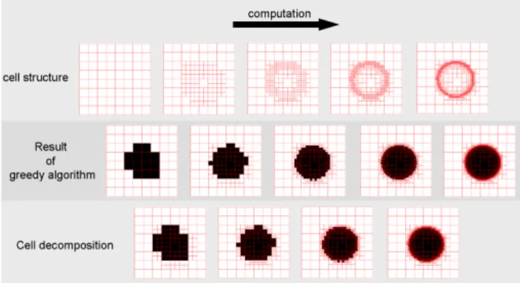
In previous algorithm, the partition of unit square [0, 1]2 is given a-priori but after the computation, the final shape S can provide an idea about where it could be useful to refine the partition by splitting some cells in smaller ones. It leads to following algorithm where the previous greedy algorithm is used as routine and where the partition of cells is updated at each step (Fig. 4):
• Initialization:choose an initial cell decomposition of [0, 1]2 as for instance in 64 squares of size 0.125 ×
0.125.
• Repeat: Perform Greedy Algorithm and provide a shape S. Split all cells of the inside and outside boundary of S.
• End: Stop when the number of cells becomes too large or if the variation of the error sum becomes insignificant.
Fig. 4. The principle of the algorithm is to update the partition of cells by decomposing at each step the cells of the boundary of the shape. Then we restart the greedy algorithm as a routine to compute a new shape, and so one until the time of computation is expired or until stability.
In order to avoid an exponential growing of the number of cells, we choose in practice to bound the minimal size of the cells: we fix a-priori a minimal area under which cells are no more divided because they would be too small. The consequence is also to make the partition of cells convergent -the algorithm ends when there are no more changes between two steps- but it is not necessary to wait stability (2 hours on phantom 1) to provide a convenient result. In the experimental section, this algorithm has been tested with quad-trees.
C. Multiresolution Probabilistic Algorithm
The algorithm that we present here is close to Simulated Annealing (SA) [10]. In SA, a current state S is modified randomly with a probability of change which is related to the input by an energy term E(S) and which decreases with the time. More precisely, at each step, the algorithm generates randomly a new state S0 by some small modifications of S. The state S0 is accepted as new current state with a probability eE(S0 )−E(S)T (1 if E(S0) ≥ E(S)) where T is a
global parameter called temperature that decreases during the time. The repetition of this process several times is inspired by the method of annealing in metallurgy where a material is heated and cooled several times in order to improve its quality. In our framework, the energy term is Errora(S) since it is
the value that we want to minimize. The fact that we suggest a variant of Simulated Annealing rather than the classical algorithm itself comes from the decomposition of this energy inP
k∈KAEa(Ck). It allows to work locally: instead of trying
a small change on S and computing the global energy variation to determine the probability to accept it, we perform a lot of small changes in parallel and accept each one of them with a probability that depends on local criterion and of temperature. It is a win of time, but there is of course a small drawback: several local changes can be accepted in parallel at different places although they have together a negative effect on the total energy. Nevertheless, we can hope that it does not occur too often, and there is also a most important reason to replace
the classical criterion of acceptance in eE(S0 )−E(S)T : our goal is
not only to find the best allocation of colors to each cell but also to improve the cell partition in order to provide a high resolution on the boundary of the result. It means that our current state is not only S, but S and the partition. It follows that among the possibilities to find a new current state, there is the possibility to change the color of a cell but also to split it or to merge neighbors with the same color. This change of the structure does not modify the energy, but it should also be guided by some probabilistic criterion.
After these general considerations, let us give briefly the details of the algorithm:
• Initialization:choose an initial cell decomposition of [0, 1]2 as for instance in 64 squares of size 0.125 ×
0.125. Compute a current state S with the greedy algorithm.
• Repeat 1:Take a (high) temperature T = T0.
◦ Repeat 2: For all cells of [0, 1]2, consider three possibilities of change: split, merge with its neighbors, change its color and accept it randomly with a given probability threshold. Decrease temperature.
◦ End of Repeat 2:Temperature is 0.
• End:Maximal time of computation has been reached. For a cell Ck, the probability to merge with its neighbors
(in the multiresolution data structure) is 0 if their colors are different. Otherwise, it depends only on the temperature with
p(mergeCk) = p0
|M E(Ck)|
AE(Ck)
eαT
with a negative α and a parameter p0 (in next experiments
p0= 0.05). The probability to split Ck in smaller cells is
p(splitCk) = p1(1 −
|M E(Ck)|
AE(Ck)
)eαT
with a parameter p1 (in next experiments p1 = 1). An area
factor can be added in order to favor the split of the large cells. If the absolute energy is null, X-areas are correct, then we don’t split the cell. We can also notice that with the factor 1 −M E(Ck)
AE(Ck), we tend to split the cells where the mean error
is close to 0, namely where in some strips there is a lack of black while others it is an excess. For the change of color, the probability to become black is a growing function of the ratio
M eanEnergy(Ck)
AbsoluteEnergy(Ck), for instance
p(Ck → black) = p2
M E(Ck)
AE(Ck)
eαT
if the mean energy is positive (it expresses a lack of black). The probability for a cell to become white is symmetric. Of course, we describe here a heuristic in which parameters can be hard to find. There is a balance to find between merging and splitting, with of course a minimal size for splitting. The evolution of the solution is guided by basic principles which was the main point of this work. More sophisticated criterion can be introduced. If all the neighbors of a cell are black while the cell is white, we have for instance increased the coefficient p2 in order to try to regularize the colors of the solution, but
such an a-priori has also the drawback to reduce the research of a solutions in some directions.
V. EXPERIMENTS
A. Experimental Protocol
We have tested the Greedy Algorithm (we notice it GA), the Greedy Algorithm with Multiresolution Enhancement (GAME) and the Multiresolution Probabilistic Heuristic (MPH) (with several minimal areas for the cells) on the same phantom images with the same protocol on a laptop with a dual core at 2.80 Ghz with 4 Gb of RAM: The exact X-areas of the phantom are computed and then introduced as input of each algorithm. The criterion which allows to evaluate the quality of the result S is the error sum Errora(S). We
choose to report for each algorithm the graphics of the error index (104number of directionsErrorSum(S) ) in function of the time of computation (Fig. 6) for some chosen phantoms. Notice that if you take the X-areas of an image of resolution 100 × 100 and just change the color of one pixel, the error index of the new image according to the X-areas of the initial image is 1. • This presentation of the results is consistent for the multiresolution algorithms GAME and MPH: we run the algorithm only one time and register the evolution of the error during the computation. A curve comes from only one iteration of the algorithm.
• The results are more artificial in the case of the greedy algorithm without multiresolution GA since its main parameter is the resolution of the resulting image: then we try several resolutions and report for each its time of computation and the error sum of the result. In this case, each point corresponds to one iteration of GA and the whole curve corresponds to many.
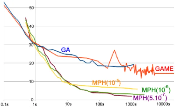
We illustrate the results with two phantoms - a basic one (Fig. 5) and a more complex one (Fig. 7). First phantom has been reconstructed from 3 directions and 128 sensors (Fig. 5 and 6). With several minimal areas for the nodes (10−5, 10−6 and 5.10−7), we can notice that decreasing this value allows to provide better results with multiresolution. There is however a limit of 200000 cells due to the memory size which does not allow to go further. Second phantom has been reconstructed with 12 directions and 128 sensors since its shape is more complex (Fig. 7 and 8). Results are drawn with a logarithmic scale for the time.
B. Interpretation of the results
For phantom 1, the multiresolution algorithms MPH out-performs the greedy algorithms GA and GAME. It requires less time for a better result. Notice that with phantom 1 and 12 directions instead of 3, GA provides lower error indices than GAM E and becomes close to M P H. The greedy algorithm GA is very sensitive to the number of directions. Then, it is not really surprising that on the second phantom -the flowers-the simple greedy algorithm provides a better final result since MPH is stopped due to the limited size of memory, which is a bit frustrating.
VI. CONCLUSION
The experimental results show that elementary algorithms provide results of good quality with only few directions if the shape in not too much complicated. The second point is that
Fig. 5. Phantom 1 - A: the first phantom. B: the result of greedy algorithm GA with resolution 400 × 400, which makes 160000 cells or pixels with an error index around 18. C: the result with multiresolution of GAME with an error index of 14.3 and 25854 cells at the end. D: the result of the probabilistic algorithm MPH with minimal area 10−5 (better results are obtained with 10−6and 5.10−7). Error index is 5.8 with 25517 cells.
Fig. 6. Results on phantom 1 - In abscissas, the time of computation is given on a logarithmic scale. The ordinate is the error index (a value of 1 corresponds to one pixel with a resolution 100 × 100). The error index of GA reaches 18 while GAME, with a minimal area of 10−5 reaches 14.3 with 25854 cells. Algorithm MPH with three different minimal areas (10−5, 10−6and 5.10−7) outperforms the other algorithms with, respectively, error indices 5.8, 2.9, 1.9 for 25517, 60919, 181969 cells.
multiresolution heuristics turn out to be a promising approach with fast results for the class of problems that we consider.
REFERENCES
[1] R. J. Gardner, Geometric Tomography, ser. Encyclopedia of Mathemat-ics and its Applications. Cambridge University Press, 1995. [2] J. Radon, “Uber die bestimmung von funktionen durch ihre
integralw-erte langs gewisser mannigfaltigkeiten,” Berichte ¨uber die Verhandlun-gen der K¨oniglich-S¨achsischen Akademie der Wissenschaften zu Leipzig, Mathematisch-Physische Klasse, vol. 69, pp. 262–277, 1917. [3] R. N. Bracewell, “Strip integration in radio astronomy,” Australian
Journal of Physics, vol. 9, no. 2, pp. 198–217, 1956.
[4] J. Zhu, X. Li, M. Ye, and G. Wang, “Analysis on the strip-based pro-jection model for discrete tomography,” Discrete Applied Mathematics, vol. 156, no. 12, pp. 2359–2367, 2008.
Fig. 7. Phantom 2 - A: the second phantom. B: the result of greedy algorithm GA with resolution is 520 × 520 which makes 270400 pixels with an error index around 4.4. C: the result of GAME with minimal area 10−5: the error index of 11.4 with 69457 cells. D: the result of the MPH with minimal area 10−5has an error index of 14.3 with 120214 cells.
Fig. 8. Results on phantom 2 - The error index of GA reaches 4.4 while GAME, with a minimal area of 10−5reaches 11.4 with 69457 cells. Algorithm MPH with minimal area 10−5 stops with an error of 14.3 and 120214 cells due to the memory limit.
[5] K. J. Batenburg, W. Fortes, L. Hadju, and R. Tijdeman, “Bounds on the difference between reconstructions in binary tomography,” in Proc. of the 16th IAPR international conference on Discrete Geometry for Computer Imagery, Nancy, France, 2011, pp. 369–380.
[6] S. Bonnet, F. Peyrin, F. Turjman, and R. Prost, “Multiresolution reconstruction in fan-beam tomography,” IEEE Transactions on Image Processing, vol. 11, no. 3, pp. 169–176, 2002.
[7] Y. D. Witte, J. Vlassenbroeck, and L. V. Hoorebeke, “A multiresolution approach to iterative reconstruction algorithms in x-ray computed tomography,” IEEE Transactions on Image Processing, vol. 19, no. 9, pp. 2419–2427, 2010.
[8] C. Soussen and A. Mohammad-Djafari, “Approche multirsolution pour la reconstruction 3d de dfaut en tomographie x,” in Proc. of GRETSI, Vannes, France, 1999, pp. 1197–1200.
[9] R. Finkel and J. Bentley, “Quad trees: A data structure for retrieval on composite keys,” Acta Informatica, vol. 4, no. 1, pp. 1–9, 1974. [10] S. Kirkpatrick, C. Gelatt, and M. Vecchi, “Optimization by simulated
![Fig. 3. Patterns of the partition of the domain of interest [0, 1] 2 in polytopes. We cut again it with respectively 8 (left), 16 (right) directions with 8 strips of width 0.125 which turn around the center of the square and count the number of polytopes i](https://thumb-eu.123doks.com/thumbv2/123doknet/14600269.543888/4.892.59.443.168.366/patterns-partition-domain-polytopes-respectively-directions-strips-polytopes.webp)