HAL Id: tel-00822114
https://tel.archives-ouvertes.fr/tel-00822114
Submitted on 14 May 2013
HAL is a multi-disciplinary open access
archive for the deposit and dissemination of sci-entific research documents, whether they are pub-lished or not. The documents may come from teaching and research institutions in France or abroad, or from public or private research centers.
L’archive ouverte pluridisciplinaire HAL, est destinée au dépôt et à la diffusion de documents scientifiques de niveau recherche, publiés ou non, émanant des établissements d’enseignement et de recherche français ou étrangers, des laboratoires publics ou privés.
Initialize and Calibrate a Dynamic Stochastic
Microsimulation Model : application to the SimVillages
Model
Maxime Lenormand
To cite this version:
Maxime Lenormand. Initialize and Calibrate a Dynamic Stochastic Microsimulation Model : applica-tion to the SimVillages Model. Other. Université Blaise Pascal - Clermont-Ferrand II, 2012. English. �NNT : 2012CLF22315�. �tel-00822114�
N˚ d’ordre : D.U. 2315 EDSPIC : 597
UNIVERSITÉ BLAISE PASCAL - CLERMONT II
ÉCOLE DOCTORALE
SCIENCES POUR L’INGÉNIEUR DE CLERMONT-FERRAND
THÈSE
Présentée par
M
AXIME
LENORMAND
Master Statistiques et Traitement des Données pour obtenir le grade de
DOCTEUR D’UNIVERSITÉ
SPÉCIALITÉ : Informatique
Initialize and Calibrate a Dynamic Stochastic
Microsimulation Model:
Application to the SimVillages Model
Soutenue publiquement le 12 décembre 2012 devant le jury composé de :Président : Laurent SERLET
Professeur des universités, Université Blaise-Pascal, Clermont-Ferrand
Rapporteurs : Jean-Pierre NADAL
Directeur de recherche, CNRS, Paris
Philippe TOINT
Professeur des universités, Université de Namur (FUNDP), Namur
Examinateurs : Marc BARTHELEMY
Chercheur, Institut de Physique Theorique, Gif-sur-Yvette
Jean-Michel MARIN
Professeur des universités, Université Montpellier 2, Montpellier
Directeur de thèse : Guillaume DEFFUANT
Directeur de recherche, Irstea, Clermont-Ferrand
Invitée : Sylvie HUET
Acknowledgement
Je tiens tout d’abord à remercier Sylvie Huet et Guillaume Deffuant pour avoir su me guider tout au long de ces trois années. Sylvie, merci pour tes conseils, ta patience, ta disponibilité et aussi pour ton pif incroyable capable de repérer (ou de tomber ma-lencontreusement sur) le moindre bug présent dans un code ou un article. Guillaume, merci de m’avoir accordé un peu de ton temps si précieux, merci pour l’aide que tu m’as apportée, la confiance que tu m’as donnée et pour les longues heures que tu as passées sur nos articles et sur mon manuscrit. Je vous remercie tous les deux d’avoir trouvé le juste équilibre entre encadrement et autonomie. Trouvez dans ces quelques lignes le témoignage de ma profonde gratitude. Merci pour tout.
Mes remerciements vont également à Floriana Gargiulo avec qui c’est un réel plaisir de travailler, j’espère que nous continuerons à collaborer ensemble dans les années futures.
Je tiens à remercier mon "esclave", comme il se qualifie lui même, l’informatismique Nicolas Dumoulin sans qui ma thèse aurait duré trente années au lieu de trois. Un grand merci à toi Nico !!
Merci également aux membres de mon comité de thèse Timoteo Carletti, Didier Blanchet, Hervé Monod, Fabien Campillo et plus particulièrement merci à Franck Jabot pour sa contribution à ma thèse.
Mes remerciements vont également à Jean-Pierre Nadal et Philippe Toint qui ont accepté d’être rapporteurs de cette thèse. Je remercie aussi les autres membres du jury Marc Barthélémy, Jean-Michel Marin et Laurent Serlet.
Merci également à tous les membres du Lisc. En particulier, merci à Clairus, Wei Wei, Bruni et JD.
Mes remerciements suivants vont à l’ensemble des membres du projet PRIMA. En particulier je tiens à remercier Olivier Aznar, Eliska Kozáková, Omar Baqueiro Espinosa, Olivier Barreteau, Mario Njavro et Marian Raley.
Résumé Etendu
L’objectif de ce travail est de développer des outils statistiques et des modèles in-formatiques pour initialiser et calibrer les modèles de microsimulation dynamique sto-chastique. Nous avons développé ces outils et modèles dans le cadre de l’élaboration du modèle SimVillages, certains développements sont très spécifiques à ce modèle, d’autres plus génériques.
L’hypothèse à la base de la microsimulation est que se placer au niveau de l’individu donne plus de chance de comprendre ce qui se passe à un niveau plus agrégé. C’est dans cette optique que l’on utilise la microsimulation dynamique. L’idée est de créer une société virtuelle où l’individu est l’entité à la base du système. Cette société virtuelle devra être statistiquement semblable à la société "réelle" sur les indicateurs qui nous intéressent, définis en fonction des objectifs du modèle. On fait ensuite évoluer cette société dans le temps en essayant de reproduire les faits passés pour comprendre com-ment ils se sont produit et ainsi tenter d’anticiper l’avenir. Mais pour créer un tel modèle informatique plusieurs questions se posent. Tout d’abord comment créer la population synthétique de base du modèle en absence de donnée détaillée sur la population à re-produire ? Comment extraire l’information des données pour construire la dynamique du modèle ? Si il existe des paramètres du modèle inconnus, comment estimer leurs va-leurs ? Ce travail est consacré à ces questions.
Dans ce résumé étendu, je présente, dans un permier temps, le modèle de micro-simulation dynamique SimVillages servant de cadre applicatif aux travaux de la thèse dans le but de donner aux lecteurs une idée plus précise du contexte dans lequel s’ins-crivent les développements méthodologiques présentés. Dans un second temps, je pré-sente un résumé des chapitres.
Le modèle de microsimulation SimVillages
Le modèle de microsimulation dynamique stochastique SimVillages a été développé
durant le projet Européen PRIMA1. Son objectif est de permettre de mieux comprendre
les différences d’évolution des municipalités rurales. Dans ce modèle, on fait l’hypo-thèse que l’évolution de ces communes dépend, d’une part, des interactions entre municipalités à travers le navettage et la consommation de service et d’autre part du nombre d’emplois dans les différents secteurs d’activité (fixé de manière exogène à l’aide de scenarios) et d’emplois de services de proximité (supposés dépendant des ca-ractéristiques de la municipalité).
Le modèle SimVillages appartient à la famille des modèles de microsimulation. Les origines de l’approche par microsimulation remontent à la fin des années cinquante (Orcutt,1957). Elle est la première approche à avoir pris en compte le niveau individuel dans la modélisation des systèmes complexes mais elle fait maintenant partie d’une
1PRototypical policy Impacts on Multifunctional Activities in rural municipalities - EU 7th Framework
vi Résumé Etendu
famille plus large de modèle : les modèles individus-centré. Cette famille de modèles regroupe la microsimulation, la théorie des jeux, les automates cellulaires, les
simula-tions orientées-objet et les simulasimula-tions multi-agents (Amblard,2003). Les modèles de
microsimulation modélisent à un niveau microscopique (à l’échelle de l’individu) un système complexe, ils sont dynamiques lorsqu’ils évoluent dans le temps et stochas-tiques lorsqu’ils sont composés d’une part d’aléa rendant chaque résultat du modèle "unique". L’intérêt de ce type de modèle est la flexibilité des résultats. En effet, le fait de travailler à une échelle très fine permet d’obtenir des résultats à plusieurs niveaux d’agrégation. Cependant, la microsimulation se voit opposer plusieurs critiques : le vo-lume de données requis, le temps de calcul et la stochasticité. Depuis la première vision
d’Orcutt avec DYNASIM (Orcutt et al.,1976) de nombreux modèles de microsimulation
dynamique ont été proposés tels que DESTINIE (INSEE,1999) ou encore LifePaths
(Sta-tistics Canada, 2004). Ces modèles permettent d’analyser l’évolution de systèmes com-plexes en prenant en compte une hétérogénéité dérivée des observations des individus et de leurs interactions. Le modèle SimVillages est stochastique incluant des objets hé-térogènes (individus, ménages, municipalités, emplois, logements,...) et ses propriétés ne peuvent pas être dérivées analytiquement, nous avons besoin de réaliser un grand nombre de simulations pour comprendre son fonctionnement et ajuster les valeurs de paramètres inconnus pour obtenir une bonne adéquation entre données observées et données simulées.
Le modèle SimVillages est un système dynamique à temps discret Xt+1= M (θ ,γ,
Xt) où Xt∈ Rnest l’état du système,γ = (γ1, ...,γm) les paramètres fixés du modèle et θ =
(θ1, ...,θp) les paramètres inconnus du modèle. On observe des trajectoires de ce système
dynamique, à partir de conditions intitiales X0et pendant un certain nombre de pas de
temps T . Dans le modèle SimVillages un pas de temps équivaut à un an. Nous pouvons
observer sur laFigure 1que le modèle commence en 1990 et que pour le confronter à la
réalité nous disposons de deux dates de recensement, 1999 et 2006. Nous pouvons aussi
observer que pour des valeurs fixées de X0,γ et θ chaque éxecution du modèle donne
des trajectoires différentes à cause de la stochasticité.
Il existe deux catégories de paramètres, les paramètres fixés du modèleγ et les
pa-ramètres inconnus du modèleθ . Les paramètres fixés du modèle sont à configurer par
l’utilisateur, leur valeur est dérivée de valeurs et de distributions de probabilité extraites des données observées à l’aide de méthodes statistiques et de traitement de données. Elles peuvent aussi prendre la forme de scenario intervenant de manière exogène dans la simulation. L’état initial fait aussi partie des paramètres fixés du modèle, il est re-présenté par une population synthétique construite à partir des données observées, à l’échelle de la région considérée. Chaque individu de cette population est caractérisé par :
• un ménage dont il fait partie, d’une certaine taille (de 1 à 6 ou plus individus) et d’un certain type (personne seule, famille monoparentale, couple avec enfant(s), couple sans enfant(s) et autre ménage),
Résumé Etendu vii
• une situation au regard de l’emploi (employé, sans-emploi, retraité, inactif ou étu-diant),
• une catégorie socio-professionnelle s’il est actif (agriculteur, artisan, profession intermédiaire, cadre, employé et ouvrier),
• un lieu de travail s’il est actif occupé (dans une commune de la région ou à l’exté-rieur de la région) et un secteur d’activité (agriculture, industriel ou service).
Une représentation des entités composant l’état initial du modèle est proposée
Fi-gure 2. Il est important que cet état initial soit statistiquement le plus proche possible de la population observée car il est le point de départ pour la calibration. En effet, l’état initial a un impact sur les évolutions futures du modèles.
Les paramètres inconnus du modèle sont ceux que nous n’avons pas pu
directe-ment extraire des données. Nous pouvons observer sur laFigure 3que les paramètres
inconnus du modèle sont extraits des données via une procédure de calibration tandis que les paramètres fixés du modèle sont directement extraits des données. La calibra-tion du modèle SimVillages ne peut se faire analytiquement. Pour calibrer le modèle, nous faisons donc varier les paramètres pour minimiser une fonction cible, distance entre des statistiques construites à partir des données observées et des données simu-lées (population moyenne...). Nous devons pour cela parcourir efficacement l’espace des paramètres afin de trouver le ou les jeux de valeurs de paramètres minimisant la cible. Cela nécessite un grand nombre de simulations du modèle. Par exemple, sur la
Figure 1, le but est de trouver des valeurs deθ qui ont au moins une trajectoire "proche" des données observées (représentées par les points verts).
Du point de vue de la dynamique du modèle, à chaque pas de temps, la population des communes évolue, les individus font des choix de vie, d’étude, de carrière, d’union, peuvent avoir des enfants, divorcer, migrer et mourir. Le modèle prend en compte, de manière endogène, les migrations inter-communales, les créations ou les suppressions d’emplois dans les services de proximité en fonction du nombre d’habitant. En plus de ces évolutions endogènes on introduit des scenarios représentant les décisions poli-tiques prises au niveau régional telles que, par exemple, l’implantation d’une entreprise sur une commune. Ces scenarios modifient de manière exogène l’évolution des com-munes.
La région d’étude modélisée avec le modèle SimVillages est le département français du Cantal qui possédait 158 723 habitants répartis en 260 communes en 1990. Le modèle a pour point de départ 1990 et l’estimation de la distribution de valeurs des paramètres a été effectuée en deux points dans le temps, 1999 et 2006 (années correspondant au recensement de la population effectué par l’INSEE). Une simulation sur un ordinateur de bureau prend environ une minute. Une description complète du modèle est détaillée dansHuet et al.(2012a) et sa paramétrisation est détaillée dansHuet et al.(2012b)
viii Résumé Etendu
Résumé des chapitres
Ce travail de thèse se divise en quatre chapitres. Les deux premiers chapitres portent sur l’initialisation du modèle SimVillages avec la création d’une population synthétique. Le troisième chapitre concerne un modèle statistique permettant d’estimer le nombre d’emplois dans les services de proximité. Le quatrième chapitre présente une méthode de calcul bayésien approché permettant d’estimer la distribution des valeurs des para-mètres inconnus du modèle.
DansLenormand and Deffuant(2012), présenté dans leChapitre 1, nous avons tout
d’abord implémenté l’algorithme proposé parGargiulo et al.(2010) pour créer une
po-pulation synthétique de l’Auvergne en 1990. Ensuite, nous validons cette popo-pulation et nous comparons l’algorithme utilisé avec la méthode Iterative Proportional Updating
(IPU) proposé parYe et al.(2009). L’intérêt de l’algorithme proposé dansGargiulo et al.
(2010) est qu’il n’utilise que des données agrégées palliant ainsi l’absence d’un
échan-tillon représentatif de la population. Nous montrons dans le premier chapitre que cet algorithme est plus rapide et qu’il donne de meilleurs résultats que l’autre algorithme utilisant un échantillon. En contre partie il nécessite plus de temps dans la préparation des données.
Pour finaliser la population synthétique il a fallu assigner à chaque individu actif occupé de cette population un lieu de travail lorsqu’il travaillait à l’extérieur de sa com-mune de résidence. Le réseau formé par les interactions entre comcom-munes pour les dé-placements domicile-travail s’appelle un réseau de navettage. Les données détaillées étant indisponible en 1990 il a fallu développer un algorithme de génération de réseaux de navettage permettant de simuler un réseau à partir de données agrégées. Ce
mo-dèle a été proposé dansGargiulo et al.(2012) (disponible enAnnexe B), cet algorithme
construit le réseau progressivement, en attribuant aux navetteurs, un par un, un lieu de travail avec une probabilité d’accepter ce lieu de travail qui augmente avec l’offre d’em-ploi de ce lieu de travail et diminue avec la distance entre la commune de résidence et la commune de travail candidate. Ce modèle a ensuite été adapté à 34 régions de France (Lenormand et al.,2012b). Dans cet article, disponible enAnnexe C, une généralisation du modèle de base est proposée en incluant l’extérieur de la région (possibilité pour les navetteurs de travailler hors de la région d’étude) et en comparant plusieurs fonctions
de décisions pour modéliser l’effet de la distance (puissance et exponentielle). Dans
Le-normand et al.(2012c), présenté dans leChapitre 2, nous proposons une loi permettant d’estimer le seul paramètre du modèle en fonction des caractéristiques de la région étu-diée, cette loi a été testée et validée sur 80 régions d’Europe et d’Amérique.
Dans leChapitre 3nous présentons un modèle statistique permettant d’estimer le
nombre d’emplois dans les services de proximité d’une commune en fonction de ses caractéristiques. Dans un premier temps, nous avons essayé d’estimer, pour une com-mune, la présence ou l’absence de service de proximité mais aussi le nombre d’emplois
dans ces différents services en fonction des caractéristiques de la commune (voir
An-nexe D). Malgré des résultats satisfaisants, ce travail était trop compliqué à mettre en œuvre dans le modèle SimVillages car il était difficile de sélectionner les services des-tinés à la population sachant que certains services ne servent qu’en partie à la
popu-Résumé Etendu ix
lation locale. DansLenormand et al.(2012a), présenté dans le troisième chapitre de la
thèse, nous proposons une méthode permettant d’estimer, pour une commune donnée, le nombre d’emplois dans les services de proximité en fonction du nombre d’habitants et de son voisinage en terme de service.
Pour estimer la distribution des valeurs des paramètres inconnus du modèle, nous
proposons dansLenormand et al.(2012d), présenté dans leChapitre 4, un algorithme
de calcul Bayésien approché (ABC) par échantillonage préférentiel. Les méthodes d’échantillonage préférentiel appliquées à l’ABC sont dérivées de méthodes d’échan-tillonnage classique et elles sont considérées comme étant les plus efficaces en termes de temps de calcul parmi les méthodes ABC. Nous étudions les paramètres de notre algorithme et nous l’avons comparé à trois algorithmes concurrents dans la littérature. Nous montrons qu’avec n’importe quelle paramétrisation de notre algorithme, nous prenons de 2 à 8 fois moins de simulations pour atteindre au moins la même qualité de résultats que les trois autres algorithmes.
Mots-clés : Microsimulation, Modèle Complexe, Modèle Individus Centré, Modèle Stochastique, Calibration, Initialisation, Population Synthétique, Iterative Proportional Updating, Modèle de Réseaux de Navettage, Modèle de Déplacement, Loi de Gravité, Mobilité Humaine, Réseau Spatial, Besoin Minimal, Service de Proximité, Régression Quantile, Municipalité Rurale, Calcul Bayésien Approché, Population Monte Carlo, Se-quential Monte Carlo.
Abstract
The purpose of this thesis is to develop statistical tools to initialize and to cali-brate dynamic stochastic microsimulation models, starting from their application to the SimVillages model (developed within the European PRIMA project). This model in-cludes demographic and economic dynamics applied to the population of a set of rural municipalities. Each individual, represented explicitly in a household living in a mu-nicipality, possibly working in another, has its own life trajectory. Thus, model includes rules for the choice of study, career, marriage, birth children, divorce, migration, and death.
We developed, implemented and tested the following models:
• a model to generate a synthetic population from aggregate data, where each in-dividual lives in a household in a municipality and has a status with regard to employment. The synthetic population is the initial state of the model.
• a model to simulate a table of origin-destination commuting from aggregate data in order to assign a place of work for each individual working outside his munici-pality of residence.
• a sub-model to estimate the number of jobs in local services in a given municipal-ity in terms of its number of inhabitants and its neighbors in terms of service. • a method to calibrate the unknown SimVillages model parameters in order to
satisfy a set of criteria. This method is based on a new Approximate Bayesian
Computation algorithm using importance sampling. When applied to a toy
example and to the SimVillages model, our algorithm is 2 to 8 times faster than the three main sequential ABC algorithms currently available.
Keywords: Microsimulation, Complex Model, Individual Based Models, Stochastic Models, Calibration, Initialisation, Synthetic Population, Sample-Free, Iterative Pro-portional Updating, Network Generation Models, Commuting Patterns, Commuting Networks, Gravity Law, Human Mobility, Spatial Networks, Minimum Requirement, Proximity Service Jobs, Quantile Regression, Rural Municipality, Approximate Bayesian Computation, Population Monte Carlo, Sequential Monte Carlo.
Preamble
This research has been motivated and partly funded by the European project PRIMA (PRototypical policy Impact on Multifonctional Activities in rural municipalities col-laborative project, European Union 7th Framework Programme (ENV 2007-1)). This project aimed at developing a method for scaling down the analysis of policy impacts on multifunctional land uses and on the economic activities. It developed a microsim-ulation model, called SimVillages, designed and validated at municipality level, using input from stakeholders. The model address the structural evolution of the populations (appearance, disappearance and change of agents) depending on the local conditions for applying the structural policies on a set of municipality case studies.
This PhD thesis was carried out between January 2010 and December 2012 in the Lab-oratory of Engineering for Complex System (LISC) in National Research Institute of Sci-ence and Technology for Environment and Agriculture (IRSTEA) located in Clermont-Ferrand. The LISC develops individual-based models to study the complexity of social or eco-system dynamics and new methods for assessing the viability or resilience of such systems. In the PRIMA project, the LISC has developed the SimVillages model for the Auvergne case study, and this model has then been adapted to other case studies in the UK and Germany.
This PhD thesis was supervised by Guillaume DEFFUANT (Head of LISC) and Sylvie HUET (Engineer).
Each chapter of this PhD thesis is a paper submitted or accepted in a peer reviewed international journal.
Contents
Résumé Etendu v
Abstract xi
Preamble xiii
Contents xvii
List of Figures xix
List of Tables xxi
List of Algorithms xxiii
Introduction 1
Overview . . . 1
The SimVillages microsimulation model . . . 1
Structure of thesis . . . 5
1 Generating a Synthetic Population of Individuals in Households 9 1.1 Introduction. . . 10
1.2 Details of the chosen methods. . . 11
1.2.1 Sample-free method. . . 11
1.2.2 The sample-based approach. . . 13
1.3 Generating a synthetic population of reference . . . 13
1.3.1 Generation of the individuals . . . 15
1.3.2 Generation of the households. . . 15
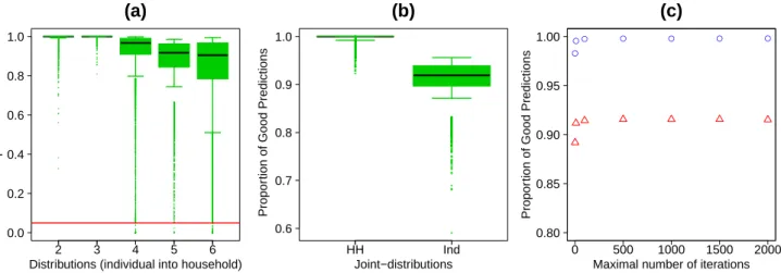
1.3.3 Distributions for affecting individual into household . . . 15
1.4 Comparing sample-free and sample-based approaches . . . 16
1.4.1 Fitting accuracy measures . . . 18
1.4.2 Sample-free approach . . . 18
1.4.3 Iterative Proportional Updating . . . 19
1.5 Discussion . . . 21
References . . . 22
2 A Universal Model of Commuting Networks 25 2.1 Introduction. . . 26
2.2 The model . . . 27
2.3 A universal law ruling parameterβ . . . 28
2.4 Comparaison with other universal derivations of commuting networks. . . 32
2.5 Discussion . . . 33
xvi Contents
Appendix 2.A: Data description. . . 37
Appendix 2.B: Results with standard indicators of error . . . 40
3 Deriving the Number of Jobs in Proximity Services 43 3.1 Introduction. . . 44
3.2 Material and methods. . . 45
3.2.1 The data from the French statistical office . . . 45
3.2.2 Model estimate of the number of jobs in proximity services . . . 46
3.3 Results. . . 48
3.4 Discussion . . . 50
References . . . 51
4 Adaptive Approximate Bayesian Computation for Complex Models 53 4.1 Introduction. . . 54
4.2 Adaptive population Monte-Carlo ABC . . . 55
4.2.1 Overview of the APMC algorithm . . . 55
4.2.2 Weights correcting the kernel sampling bias . . . 56
4.2.3 The stopping criterion . . . 57
4.3 Experiments on a toy example. . . 57
4.3.1 Particle duplication in SMC and RSMC . . . 58
4.3.2 Influence of parameters on APMC. . . 58
4.3.3 Comparing performances. . . 60
4.4 Application to the model SimVillages. . . 60
4.4.1 Model and data . . . 61
4.4.2 Study of APMC result . . . 62
4.4.3 Influence of parameters on APMC. . . 63
4.4.4 Comparing performances. . . 63
4.5 Discussion . . . 63
References . . . 65
Appendix 4.A: Description of the algorithms . . . 67
Appendix 4.B: Proof that the algorithm stops . . . 72
Summary and Perspectives 73 1 Generating a synthetic population. . . 74
1.1 Summary of my contribution . . . 74
1.2 Perspectives and open questions . . . 74
2 A universal model of commuting networks . . . 74
2.1 Summary of my contribution . . . 74
2.2 Perspectives and open questions . . . 75
3 Deriving the number of jobs in proximity services . . . 75
3.1 Summary of my contribution . . . 75
3.2 Perspectives and open questions . . . 75
4 Adaptive approximate Bayesian computation for complex models . . . 75
4.2 Perspectives and open questions . . . 76
Bibliography 79
A Parameterisation of Individual Working Dynamics 89
B Commuting Network: Getting the Essentials 115
C Generating French Virtual Commuting Network 137
D Predicting the Presence and Number of Jobs in Services 155
List of Figures
1 SimVillages model schematic representation . . . 3
2 Main components of the SimVillages model. . . 4
3 From statistics to individuals. . . 4
4 Map of the Cantal . . . 5
1.1 Results obtained with the free-sample method. . . 19
1.2 Results obtained with the sample-based method . . . 20
1.3 Maps of the average proportion of good predictions . . . 22
2.1 Three scales of geographic units . . . 27
2.2 Plot of the average CPC and the average NMAE in term ofβ . . . 30
2.3 Log-log scatter plot of the calibratedβ values in terms of average surface . 31 2.4 Common part of commuters (CPC) for the 80 case-studies . . . 34
2.5 Comparing the predictions of the radiation model with ours. . . 35
2.6 Maps to illustrate the build process regions . . . 38
2.7 NMAE and NRMSE for the 80 case-studies. . . 41
3.1 Number of service jobs per inhabitant . . . 46
3.2 Histogram of the tMFM in minutes by car in 1999. . . 47
3.3 Box-and-whisker plot of the number of service jobs per inhabitant . . . 47
3.4 Number of service jobs per inhabitant for different tMFM. . . 49
3.5 Number of proximity service jobs per inhabitant function of tMFM. . . 50
4.1 Number of distinct particles in a sample . . . 59
4.2 Posterior quality versus computing cost. . . 59
4.3 Comparing performances for the toy example . . . 60
4.4 Posterior density. . . 63
4.5 Comparing performances for the SimVillages model . . . 64
C.1 Average CPC for 23 regions . . . 146
C.2 Density of the Auvergne commuting distance distribution . . . 147
C.3 Average CPC for the power shape and the exponential shape . . . 147
C.4 Maps of the average CPC by municipalities . . . 149
C.5 Boxplots of the number of out-commuters function of the CPC. . . 150
C.6 The average calibratedβ values. . . 150
C.7 Common part of commuters for the 34 regions . . . 151
List of Tables
1.1 The Iterative Proportional Updating Table . . . 13
1.2 Data description. . . 16
1.3 Individual level attributes . . . 17
1.4 Household level attributes. . . 17
1.5 Average execution time for the two approaches . . . 21
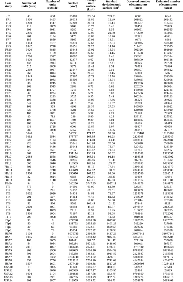
2.1 Presentation of the datasets. . . 38
2.2 Description of the case studies . . . 39
3.1 Parameter values of the quantile regression . . . 49
4.1 SimVillages parameter descriptions . . . 62
4.2 Summary statistic descriptions . . . 62
C.1 Origin-destination table for the region. . . 141
C.2 Origin-destination table . . . 145
C.3 Origin-destination table from the region to the region and the outside . . . 145
C.4 Description of the regions. . . 154
D.1 Coefficient of the GLM for each kind of service . . . 159
D.2 Percentage of good answer for each kind of service . . . 160
D.3 Coefficient of the GLM for each kind of service . . . 163
D.4 Percentage of good answer for each kind of service in 1988 and 2007 . . . . 164
List of Algorithms
1.1 The general iterative algorithm . . . 11
1.2 The iterative algorithm . . . 12
1.3 Iterative Proportional Updating algorithm . . . 14
2.1 Commuting generation model . . . 29
4.1 Likelihood-free rejection sampler 1 . . . 67
4.2 Likelihood-free rejection sampler 2 . . . 67
4.3 Population Monte Carlo ABC (PMC) . . . 68
4.4 Sequential Monte Carlo ABC Replenishment (RSMC) . . . 69
4.5 Adaptive Sequential Monte Carlo ABC (SMC). . . 70
4.6 Adaptive Population Monte Carlo ABC (APMC) . . . 71
Introduction
Contents
Overview . . . . 1
The SimVillages microsimulation model . . . . 1
Structure of thesis . . . . 5
Overview
This work aims to develop statistical tools and models to initialize and to calibrate a dynamic stochastic microsimulation model called SimVillages. Some of these tools and models are very specific to the SimVillages model, while others are more generic.
The microsimulation assumes that by considering the smallest scale brings deeper understanding of the social processes. The idea is to simulate a virtual social system where the virtual simplified individuals evolve and interact. These virtual individu-als should be defined with attributes that are statistically similar to the "real" one for the indicators of interest; these indicators being defined in terms of the model objec-tives. Then, when running this virtual system over time it should replicate past events. Analysing how the model reproduces past events, one can get some assessment of its capacity to anticipate future trends. But developing such an informatic model requires to answer several questions. How to generate a synthetic population without detailed data? If the population is organised in several spatial entities, like municipalities, how to define the relationship between them? How to extract information from data to pa-rameterize the model? If there are unknown model parameters, how to estimate their value? These are the main questions that we address in this work.
In this introduction, I first present the SimVillages microsimulation model which motivated the statistical tools developed during my PhD in order to give the reader a more precise idea of the context of the presented methodological developments. Then, I present a detailed outline of the thesis.
The SimVillages microsimulation model
The model which motivates the statistical methods developed during this PhD is the dynamic stochastic microsimulation model, SimVillages, elaborated within the
Eu-ropean PRIMA1project. This model couples demographic and economic dynamics
ap-1PRototypical policy Impacts on Multifunctional Activities in rural municipalities - EU 7th Framework
2 Introduction
plied to a population of individuals living in a set of rural municipalities. The dynamics depend, on the one hand, on the spatial interactions between municipalities through commuting flows and services, and on the other hand, on the number of jobs in various activity sectors (supposed exogenously defined by scenarios) and on the jobs in prox-imity services (supposed dependent on the size of the local population).
The SimVillages model belongs to the family of microsimulation models. The
ori-gins of the microsimulation approach date back to the late fifties (Orcutt,1957). It was
the first approach taking into account the individual level in the modeling of complex systems, but it is now part of a larger family of model: the individual-based models. This family of models includes the microsimulation, game theory, cellular automata,
simula-tions object-oriented and multi-agent simulasimula-tions (Amblard,2003). The
microsimula-tion models represent explicitly each individual of the considered populamicrosimula-tion. They are dynamic when they evolve over time and they are stochastic when they include some random processes making each model run "different". The advantage of this type of model is to provide results at different levels of aggregation. However, microsimulation has several drawbacks: the amount of data required, the computation time, and the
stochasticity. Since the first vision of Orcutt with DYNASIM (Orcutt et al.,1976) many
models of dynamic microsimulation have been proposed such as DESTINIE (INSEE,
1999) or LifePaths (Statistics Canada 2004). The SimVillages model is stochastic and
includes several types of dynamics, which make it impossible to derive its properties analytically. Therefore, it is necessary to perform numerous simulations in order to ob-serve its properties. Similarly when calibrating the model, i.e. determining the values of some parameters in order to minimise some error criterion, a systematic exploration of the parameter space is required, leading to a large number of simulations.
SimVillages is a discrete-time dynamical system Xt+1= M (θ ,γ, Xt) where Xt ∈ Rn
is the state of the system, γ = (γ1, ...,γm) the fixed parameters and θ = (θ1, ...,θp) the
unknown parameters. We observe the trajectories of the dynamical system from the
initial state X0and for a number of time steps T . In the SimVillages model a time step
is set to one year. As we can observe onFigure 1, we start the SimVillages model in 1990
and compare to census data of 1999 and 2006. Because of the stochasticity, for fixed
values of X0,γ and θ , each model run gives different trajectories.
There are two types of model parameters - the fixed parametersγ and the unknown
parametersθ . The fixed parameters are set by the user or their values are derived from
observed data using statistical methods and data analysis. They can also be part of sce-narios determined exogenously. The model’s initial state can also be considered as a fixed parameter; it is represented by a synthetic population fixed in time and built with observed data. The model is initialized with a synthetic population representing a set of municipalities. Each individual in the population is characterized by:
• a household (to which he belongs) of a certain size (from one to six or more peo-ple) and a certain type (single person, single parents, couples with child(ren) lo-cated in a municipality of the region,
The SimVillages microsimulation model 3
• a position about employment (employed, unemployed, retired, inactive or stu-dent),
• a socio-professional category (farmer, craftsman, intermediate profession, exec-utive, employee or worker) if he is active,
• a place of work (in a municipality of the region or outside of the region) and an activity sector (primary, secondary and tertiary) if he is occupied.
Xt+1 = M(θ,γ,X t) Time X X0 T 1990 Xt+1 = M(θ',γ,Xt ) θ
Θ
θ' 1999 2006Figure 1: SimVillages model schematic representation Xt+1= M (θ ,γ, Xt). The trajectories
rep-resent four runs of the SimVillages model from the initial state X0and for a number of time steps T . In red, two trajectories obtained with parameter valueθ . In blue, two trajectories obtained with parameter valueθ0. The green points represent the observed value in 1999 and 2006.
The main components of the SimVillages model are presented inFigure 2. It is
im-portant to have a statistically realistic synthetic population as an initial state because it is the starting point for calibration. Indeed, the initial state has an impact on future evolutions of the model.
The unknown model parameters are parameters that we were not able to directly
ex-tract from data. We observe inFigure 3that the unknown parameters are extracted from
data through a calibration procedure while the fixed parameters are directly extracted from data to generate the model. The SimVillages model calibration cannot be done analytically. Therefore, to calibrate the model, we vary the unknown parameters and we choose the value that minimizes a target function, defined as the distance between statistics constructed from simulated and observed data. To do this, we need to explore
4 Introduction Municipality Household Type Size Job Sector Socio-Professional Category (SPC) Housing Outside Individual Age Job Status Family Status
Figure 2: Main components of the SimVillages model
efficiently the parameter space to find the parameter values minimizing the target. This
requires a large number of model simulations. For example, inFigure 1, we need to find
θ values which have at least one trajectory "near" the observed data (represented by the
green points).
Driver instanciation depends on concrete case study – From statistics
to individuals
Available data The model
Year Population (thousands) Variation of population ( %) 1962 1 657 1968 1 592 -4,10 1975 1 481 -7,50 1982 1 438 -3,00 1990 1 262 -13,90 1999 1 121 -12,60 2007 1 010 -11,00 Effectif % Number of households which moved there since less than 10 years 200 100
Less than 2 years 46 23
from 2 to 4 years 83 41,5
from 5 to 9 years 71 35,5 Number of households
which moved there since 10 years or more 270 100
from 10 to 19 years 82 30,4
from 20 to 29 years 71 26,3
30 years and more 117 43,3
Total of households 470
1990 1999 2006
Number % Number % Number %
Farmers 60 10,8 72 15,2 44 8,3
Craftmen, storekeepers, business owners 124 22,3 50 10,5 65 12,3
Top executive managers, upper intellectual
profession 24 4,3 32 6,8 15 2,8 Intermediary professions 104 18,7 58 12,2 98 18,6 Employees 144 25,9 169 35,7 186 35,2 Workers 100 18,0 93 19,6 120 22,7 Total 556 100 474 100 528 100 2006 Number %
Number of active people working in their
municipality of residence 337 77,6
Number of active people working out of their
municipality of residence 97 22,4
Total active employed
people 434 100
generate
calibrate
Structure of thesis 5
In the dynamics of the model, at each time step, the population of municipalities evolves, individuals make choices in life about study, career, marriage. They may have children, divorce, migrate, and die. The model takes into account endogenously inter-municipal migrations and creations or destructions of jobs in local services based on the number of inhabitants. In addition to these endogenous changes, scenarios are in-troduced representing the policy decisions taken at the regional level such as the es-tablishment of a company in a municipality. These scenarios exogenously change the evolution of municipalities.
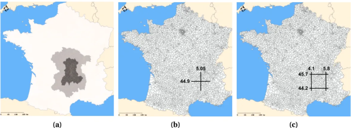
The study area modeled with SimVillages is the French department of Cantal (
Fig-ure 4), which had 158,723 inhabitants gathered in 260 municipalities in 1990. The model has for its starting point the year 1990 and the model results are evaluated in 1999 and 2006 (years corresponding to the population census conducted by the French Statistical
Institute, INSEE2). A simulation on a desktop computer takes about a minute. A
com-plete description of the model is available inHuet et al.(2012a) and the parametrization
is detailed inHuet et al.(2012b) (available inAppendix A).
Figure 4: Map to locate the Cantal departement in metropolitan France.
Structure of thesis
This thesis is divided into four chapters. The first two are dedicated to the initializa-tion of the SimVillages model. The third presents a statistical model aimed at estimating the number of jobs in proximity services. In the last one, we propose an algorithm using a Bayesian approach for estimating the posterior distribution of the unknown model parameters.
During my PhD, I implemented and validated the algorithm proposed byGargiulo
et al.(2010) that requires only aggregated data to create a synthetic population of the
6 Introduction
Auvergne French region in 1990. InLenormand and Deffuant(2012), presented in
Chap-ter 1, we compare this sample-free algorithm and a sample-based method, called
Itera-tive Proportional Updating (IPU), proposed byYe et al.(2009) for generating a synthetic
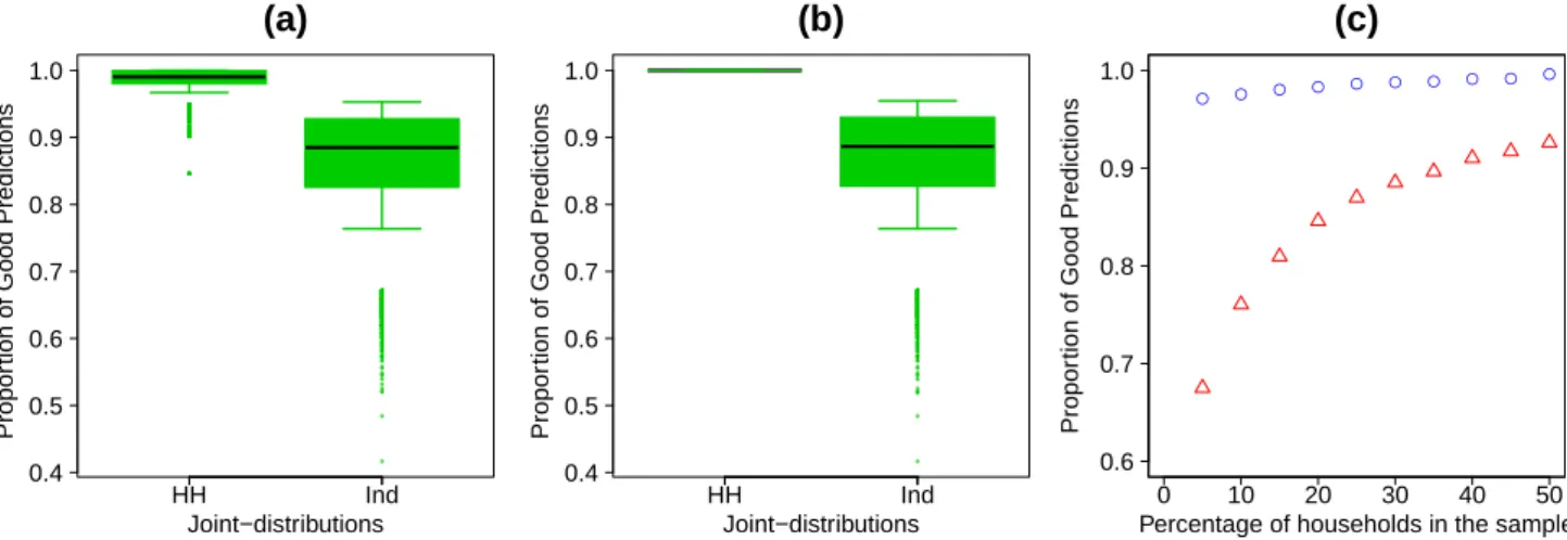
population, organized in households, from various statistics. We generate a reference population for the Auvergne region including 1310 municipalities and measure how both methods approximate it from a set of statistics derived from this reference pop-ulation. We also perform a sensitivity analysis. The sample-free method better fits the reference distributions of both individuals and households. It also demands less data but it requires more pre-processing. The quality of the results for the sample-based method is highly dependent on the quality of the initial sample.
In order to finalize the synthetic population and to create a socio-economic link with the 1310 Auvergne municipalities we needed to assign a place of work to each individual working outside his municipality of residence. The network of municipalities formed by these journeys to work is called a commuting network. Since detailed data was unavail-able in 1990 it was necessary to develop an algorithm to generate commuting networks
from aggregated data. This model was proposed inGargiulo et al.(2012) (available in
Appendix B). The model takes as input the number of commuters coming in and out of each municipality and it builds the network progressively, allocating commuters one by one in the different flows. This allocation is made according to probabilities that in-crease with the number of commuters coming to the destination, and dein-crease with the distance between the origin and destination. Then the model was adapted to 34 regions
of France (Lenormand et al., 2012b). In this paper, available in Appendix C, we
pro-pose a generalization of the model including an artificial entity representing the popu-lation located outside the considered region (offering the commuters the possibility to work outside of the region) and we propose a comparison between an exponential and
a power function to model the effect of the distance. InLenormand et al.(2012c),
pre-sented inChapter 2, we generate commuting networks on 80 case studies from different
regions of the world (Europe and United-States) at different scales (e.g. municipalities, counties, regions). We show that the single parameter of the model follows a law that depends only on the scale of the geographic units (municipality, canton, county). We show that our model significantly outperforms two other approaches proposing a
uni-versal commuting model (Balcan et al.,2009;Simini et al.,2012), particularly when the
geographic units are small (e.g. municipalities).
For the SimVillages model we have also developed a statistical model estimating the number of jobs in proximity services in a municipality. First, we have tried to estimate in a municipality the presence or absence of local services and also the number of jobs
in these different services depending on the characteristics of the municipality (see
Ap-pendix D). Despite interesting results, this work is weakened by a strong difficulty: it requires to distinguish between local and non-local services in the data and we did not
find any rigorous method to perform this task. InLenormand et al.(2012a), presented
inChapter 3, we use a minimum requirement approach (Ullman and Dacey,1960) to derive the number of jobs in proximity services per inhabitant in French rural munici-palities. We first classify the municipalities according to their time distance in minutes by car to the municipality where the inhabitants go most frequently to obtain services
Structure of thesis 7
(called MFM). For each set corresponding to a range of time distance to MFM, we per-form a quantile regression estimating the minimum number of service jobs per inhabi-tant which we interpret as an estimation of the number of proximity jobs per inhabiinhabi-tant. We observe that the minimum number of service jobs per inhabitant is smaller in small municipalities. Moreover, for municipalities of similar sizes, when the distance to the MFM increases, the number of jobs in proximity services per inhabitant increases.
To calibrate the SimVillages model, inLenormand et al.(2012d) (available in
Chap-ter 4) we proposed an approximate Bayesian computation (ABC) algorithm using
im-portance sampling (for a complete review of ABC methods seeMarin et al.(2012)). The
sampling methods applied to ABC are derived from traditional sampling methods and they are considered as the most efficients of the ABC methods in terms of computation time. This new approximate Bayesian computation algorithm aims at minimizing the number of model runs for reaching a given quality of the posterior approximation. We performed a sensitivity analysis of the parameters of our algorithm and we compared it to the three competing algorithms found in the recent literature. When applied to a toy example and to the SimVillages model, our algorithm is two to eight times faster than the three other algorithms in reaching at least the same quality of results.
To conclude, we summarize the results obtained and we present perspectives and open questions.
C
HAPTER1
Generating a Synthetic Population of
Individuals in Households:
Sample-Free vs Sample-Based
Methods
Contents
1.1 Introduction. . . . 10
1.2 Details of the chosen methods. . . . 11
1.2.1 Sample-free method. . . 11 1.2.2 The sample-based approach. . . 13
1.3 Generating a synthetic population of reference . . . . 13
1.3.1 Generation of the individuals . . . 15 1.3.2 Generation of the households. . . 15 1.3.3 Distributions for affecting individual into household. . . 15
1.4 Comparing sample-free and sample-based approaches . . . . 16
1.4.1 Fitting accuracy measures . . . 18 1.4.2 Sample-free approach . . . 18 1.4.3 Iterative Proportional Updating . . . 19
1.5 Discussion . . . . 21
References. . . . 22
Abstract. We compare a sample-free method proposed byGargiulo et al.(2010) and
a sample-based method proposed byYe et al.(2009) for generating a synthetic
tion, organised in households, from various statistics. We generate a reference popula-tion for a French region including 1310 municipalities and measure how both methods approximate it from a set of statistics derived from this reference population. We also perform sensitivity analysis. The sample-free method better fits the reference distribu-tions of both individuals and households. It is also less data demanding but it requires more pre-processing. The quality of the results for the sample-based method is highly dependent on the quality of the initial sample.
Manuscript:
Lenormand, M. and Deffuant, G. (2012). Generating a Synthetic Population of
Individ-uals in Households: Sample-Free vs Sample-Based Methods. arXiv:1208.6403v1 (Sub-mitted in Journal of Artificial Societies and Social Simulation).
10 Chapter 1. Generating a Synthetic Population of Individuals
1.1
Introduction
For two decades, the number of microsimulation models, simulating the evolution of large populations with an explicit representation of each individual, has been con-stantly increasing with the computing capabilities and the availability of longitudinal data. When implementing such an approach, the first problem is initialising properly a large number of individuals with the adequate attributes. Indeed, in most of the cases, for privacy reasons, exhaustive individual data are excluded from the public domain. Aggregated data at various levels (municipality, county,...), guaranteeing this privacy, are hence only available in general. Sometimes, individual data are available on a sample of the population, these data being chosen also for guaranteeing the privacy (for instance omitting the individual’s location of residence). This paper focuses on the problem of generating a virtual population with the best use of these data, especially when the goal is generating both individuals and their organisation in households.
Two main methods, both requiring a sample of the population, aim at tackling this problem:
• The synthetic reconstruction method (SR) (Wilson and Pownall, 1976). These
methods generally use the Iterative Proportional Fitting (Deming and Stephan,
1940) and a sample of the target population to obtain the joint-distributions of
interest (Beckman et al.,1996;Huang and Williamson,2002;Guo and Bhat,2007;
Arentze et al.,2007;Ye et al.,2009). Many of the SR methods match the observed and simulated households joint-distribution or individual joint-distribution but
not simultaneously. To circumvent these limitations Guo and Bhat(2007);
Ar-entze et al.(2007);Ye et al.(2009) proposed different techniques to match both household and individual attributes. Here, we focus on the Iterative Proportional
Updating developed byYe et al.(2009).
• The combinatorial optimization (CO). These methods create a synthetic popula-tion by zone using marginals of the attributes of interest and a sub-set of a sample
of the target population for each zone (for a complete description seeVoas and
Williamson(2000);Huang and Williamson(2002)).
Recently, sample-free SR methods appeared (Gargiulo et al.,2010;Barthelemy and
Toint,2012). These methods can be used in the usual situations where no sample is available and one must only use distributions of attributes (of individuals and house-holds). Hence, they overcome a strong limit of the previous methods. It is therefore important to assess if this larger scope of the sample-free method implies a loss of ac-curacy compared with the sample-based method.
The aim of this paper is contributing to this assessment. With this aim, we
com-pare the sample-based IPU method proposed byYe et al.(2009) with the sample-free
approach proposed byGargiulo et al.(2010) on an example.
In order to compare the methods, the ideal case would be to have a population with complete data available about individuals and households. It would allow us to mea-sure precisely the accuracy of each method, in different conditions. Unfortunately, we
Details of the chosen methods 11
do not have such data. In order to put ourseleves in a similar situation, we generate a virtual population and then use it as a reference to compare the selected methods as in
Barthelemy and Toint(2012).
In theSection 1.2we formally present the two methods. In theSection 1.3we present
the comparison results. Finally, we discuss our results.
1.2
Details of the chosen methods
1.2.1 Sample-free method
We consider a set of n individuals X to dispatch in a set of m households Y in order
to obtain a set of filled households P. Each individual x is characterised by a type txfrom
a set of q different individual types T (attributes of the individual). Each household y is
characterised by a type uy from a set of p different household types U (attributes of the
household). We define nT = {ntk}1≤k ≤qas the number of individuals of each type and
nU= {nul}1≤l ≤pas the number of households of each type. Each household y of a given
type uy has a probability to be filled by a subset of individuals L, then the content of the
household equals L, which is denoted c(y ) = L. We use this probability to iteratively fill
the households with the individuals of X .
P(c (y ) = L|uy) (1.1)
The iterative algorithm used to dispach the individuals into the households
accord-ing to theEquation 1.1is described inAlgorithm 1.1. The algorithm starts with the list of
individuals X and of the households Y , defined by their types. Then it iteratively picks
at random a household, and from its type andEquation 1.1, derives a list of
individ-ual types. If this list of individindivid-ual types is available in the current list of individindivid-uals X , then this filled household is added to the result, and the current lists of individuals and households are updated. This operation is repeated until one of the lists X or Y is void, or a limit number of iterations is reached.
Algorithm 1.1 The general iterative algorithm INPUT: X and Y
OUTPUT: P
Set P= ∅
while Y6= ∅ do
Pick at random y from Y
Pick at random L with a probability defined inEquation 1.1
if L⊂ X then P← P ∪ L Y ← Y \{y } X← X \L end if end while
12 Chapter 1. Generating a Synthetic Population of Individuals
In the case of the generation of a synthetic population, we can replace the selection of the list L by the selection of the individuals one at a time by order of importance in
the household. In this caseEquation 1.2replacesEquation 1.1.
P(x1∈ y |uy)×
P(x2∈ y |uy, x1∈ y )×
P(x3∈ y |uy, x1∈ y ,x2∈ y )×
...
(1.2)
The iterative approach algorithm associated with this probability is described in
Al-gorithm 1.2. The principle is the same as previously, it is simply quicker. Instead of generating the whole list of individuals in the household before checking it, one gener-ates this list one by one, and as soon as one of its member cannot be found in X , the iteration stops, and one tries another household.
Algorithm 1.2 The iterative algorithm INPUT: X and Y
OUTPUT: P
Set P= ∅
while Y 6= ∅ do
Pick at random y from Y
Pick at random x1with a probability P(x1∈ y |uy)
Pick at random x2with a probability P(x2∈ y |uy, x1∈ y )
Pick at random x3with a probability P(x3∈ y |uy, x1∈ y ,x2∈ y )
... if{x1, x2, x3, ...} ⊂ X then P← P ∪ {x1, x2, x3, ...} Y← Y \{y } X← X \{x1, x2, x3, ...} end if end while
In practice this stochastic approach is data driven. Indeed, the types T and U are defined in accordance with the data available and the complexity to extract the
dis-tribution of theEquation 1.2increases with nT and nU. The distributions defined in
Equation 1.2are called distributions for affecting individual into household. In concrete
applications, it occurs that one needs to estimate nT, nU and the probability
distribu-tions presented inEquation 1.2. This estimation implies that theAlgorithm 1.2can not
converge in a reasonable time because of the stopping criterion (Y 6= ∅). This stopping
criterion is equivalent to an infinite number of "filling" trials by households. In this case, we can replace the stopping criterion by a maximal number of iterations by households and then put the remaining individuals in the remaining households using relieved dis-tributions for affecting individual into household.
In a perfect case where all the data are available and the time infinite, the algorithm would find a perfect solution. When the data are partial and the time constrained, it
Generating a synthetic population of reference 13
is interesting to assess how this method manages to make the best use of the available data.
1.2.2 The sample-based approach
In this approach, proposed byYe et al.(2009), starts with a sample Ps of P and the
purpose is to define a weight wi associated with each individual and each househld
of the sample in order to match the total number of each type of individuals in X and households in Y to reconstruct P. The method used to reach this objective is the
It-erative Proportional Updating (IPU). The algorithm proposed inYe et al.(2009) is
de-scribed inAlgorithm 1.3. In this algorithm, for each type of households or individuals
j the purpose is to match the weighted sum w sj with the estimated constraints ej with
an adjustement of the weights. wi is the weight of household i in the weighted sample
and ej is an estimation of the total number of households or individuals j in P. This
estimation is done separetely for each individual and household type using a standard IPF procedure with marginal variables. When the match between the weighted sample and the constraint become stable, the algorithm stops. The procedure then generates
a synthetic population by drawing at random the filled households of Ps with
probabil-ities corresponding to the weights. This generation is repeated several times and one chooses the result with the best fit with the observed data.
Table 1.1: The Iterative Proportional Updating Table. The light grey table represents the
fre-quency matrix D showing the household (HH) type U and the frefre-quency of different individual (Ind.) types T within each filled households for the sample Ps. The dimension of D is|Ps|×(p +q),
where|Ps| is the cardinal number of the sample Ps, q the number of individual types and p the
number of household types. An element di jof D represents the contribution of filled household
i to the frequency of individual/household type j .
Filled HH
ID HH Type uuu111 · · ·· · ·· · · HH Type uuuppp Ind. Type ttt111 · · ·· · ·· · · Ind. Type tttqqq Weight 1 1 1 d11 · · · d1q d1q+1 · · ·· · ·· · · d1q+p www111 · · · · · · · · · ·· · ·· · · |Ps| |Ps| |Ps| d|Ps|1 · · · d|Ps|q d|Ps|q+1 · · · d|Ps|q+p www|P|P|Psss||| WS w sw sw s111 · · ·· · ·· · · w sw sw sppp w sw sw spp+1p+1+1 · · ·· · ·· · · w sw sw sppp+q+q+q E eee111= ˆ= ˆ= ˆnnnuuu111 · · ·· · ·· · · eeeppp= ˆ= ˆ= ˆnnnuuuppp eeeppp+1+1+1= ˆ= ˆ= ˆnnnttt111 · · ·· · ·· · · eeeppp+q+q+q= ˆ= ˆ= ˆnnntttqqq δδδ δδδ111 · · ·· · ·· · · δδδppp δδδppp+1+1+1 · · ·· · ·· · · δδδp+qpp+q+q Filled HH
ID HH Type uuu111 · · ·· · ·· · · HH Type upuupp Ind. Type ttt111 · · ·· · ·· · · Ind. Type tqttqq Weight
1 1 1 d11 · · · d1q d1q+1 · · ·· · ·· · · d1q+p www111 · · · · · · · · · ·· · ·· · · |Ps| |Ps| |Ps| d|Ps|1 · · · d|Ps|q d|Ps|q+1 · · · d|Ps|q+p www|P|P|Psss||| WS w sw sw s111 · · ·· · ·· · · w sw sw sppp w sw sw sppp+1+1+1 · · ·· · ·· · · w sw sw sppp+q+q+q E eee111= ˆ= ˆ= ˆnnnuuu111 · · ·· · ·· · · eeeppp= ˆ= ˆ= ˆnnnuuuppp eeeppp+1+1+1= ˆ= ˆ= ˆnnnttt111 · · ·· · ·· · · eeeppp+q+q+q= ˆ= ˆ= ˆnnntttqqq δδδ δδδ111 · · ·· · ·· · · δδδppp δδδppp+1+1+1 · · ·· · ·· · · δδδppp+q+q+q
1.3
Generating a synthetic population of reference for the
com-parison
Because we cannot access any population with complete data available about indi-viduals and households, we generate a virtual population and then use it as a reference
14 Chapter 1. Generating a Synthetic Population of Individuals
Algorithm 1.3 Iterative Proportional Updating algorithm INPUT: Ps,ε
OUTPUT: P
Set P= ∅
Generate D∈ M|Ps|×(p +q)(R) described by the light grey table inTable 1.1
Estimate nTand nUusing the standard IPF procedure and store the resulting estimate
into a vector E = (ej)1≤j ≤p +q as inTable 1.1
for i= 1 to |Ps| do Set wi= 1 end for for j = 1 to p +q do Compute s wj = P|Pi=1s|di jwi Computeδj =|s wej−ej| j end for Computeδ =p+q1 Ppj=1+qδj Setδmin = δ Set∆ = ε + 1 while∆ > ε do Setδprev = δ for j= 1 to p +q do for i= 1 to |Ps| do if di j6= 0 then wi=w sej jwi end if end for Compute s wj = P|Pi=1s|di jwi end for Computeδ =p+q1 Ppj=1+qδj ifδ < δmin then
Set Wopt = (wi)1≤i ≤|Ps|
δ = δmin end if
∆ = |δ − δprev|
Generating a synthetic population of reference 15
We start with statistics about the population of Auvergne (French region) in 1990 using the sample-free approach presented above. The Auvergne region is composed of 1310 municipalities, 1,321,719 inhabitants gathered in 515,736 households. In average the municipalities had about 1000 inhabitants with a minimum of 25 and a maximum of 136,180.
1.3.1 Generation of the individuals
For each municipality of the Auvergne region we generate a set X of individuals with
a stochastic procedure. For each individual of the age pyramid (distribution 1 in
Ta-ble 1.2), we randomly choose an age in the bin and then we draw randomly an activity
status according to the distribution 2 inTable 1.2.
1.3.2 Generation of the households
For each municipality of the Auvergne region we generate a set Y of households
according to the total number of individual n = |X| with a stochastic procedure. We
draw at random households according to the distribution 3 inTable 1.2while the sum
of the capacities is below n and then we determine the last household to have n equal to the sum of the size of the households.
1.3.3 Distributions for affecting individual into household
Single
• The age of the individual 1 is determined using the distribution 4 (Table 1.2).
Monoparental
• The age of the individual 1 is determined using the distribution 4 (Table 1.2).
• The ages of the children are determined according to the age of individual 1 (An
individual can do a child after 15 and before 55) and the distribution 6 (Table 1.2).
Couple without child
• The age of the individual 1 is determined using the distribution 4 (Table 1.2).
• The age of the individual 2 is determined using the distribution 5 (Table 1.2).
Couple with child
• The age of the individual 1 is determined using the distribution 4 (Table 1.2).
• The age of the individual 2 is determined using the distribution 5 (Table 1.2).
• The ages of the children are determined according to the age of individual 1 and
16 Chapter 1. Generating a Synthetic Population of Individuals
Other
• The age of the individual 1 is determined using the distribution 4 (Table 1.2).
• The ages of the others individuals are determined according to the age of individ-ual 1.
Table 1.2: Data description
ID Description Level
1 Number of individuals grouped by ages Municipality
(LAU2)
2 Distribution of individual by activity statut according to
the age
Municipality (LAU2)
3 Joint-distribution of household by type and size Municipality
(LAU2)
4 Probability to be the head of household according to the
age and the type of household
Municipality (LAU2) 5
Probability of having a couple according to the differ-ence of age between the partners (from"-16years" to "21years")
National level
6
Probability to be a child (child=live with parent) of
household according to the age and the type of house-hold
Municipality (LAU2)
To obtain a synthetic population P with households Y filled by individuals X we use theAlgorithm 1.2where we approximate theEquation 1.2with the distributions 4, 5 and 6 inTable 1.2. We put no constraint on the number of individuals in the age pyramid, hence the reference population does not give any advantage to the sample-free method.
1.4
Comparing sample-free and sample-based approaches
The attributes of both individuals and households are respectivily described in
Ta-ble 1.3andTable 1.4. The joint-distributions of both the attributes for individuals and
households give respectively the number of individuals of each individual type nT =
{ntk}1≤k ≤q and the number of households of each household type nU= {nul}1≤l ≤p. In
this case, q = 130 and p = 17. It’s important to note that p is not equal to 6 · 5 = 30
because we remove from the list of household types the inconsistent values like for ex-ample single households of size 5. We do the same for the individual types (removing for example retired individuals of age comprised betweeen 0 and 5).
Comparing sample-free and sample-based approaches 17
Table 1.3: Individual level attributes
Attribute Value Age [0,5[ [5,15[ [15,25[ [25,35[ [35,45[ [45,55[ [55,65[ [65,75[ [75,85[ 85 and more
Activity Statut Student
Active Inactive
Family Statut Head of a single household
Head of a monoparental household
Head of a couple without children household Head of a couple with children household Head of an other household
Child of a monoparental household Child of a couple with children household Partner
Other
Table 1.4: Household level attributes
Attribute Value Size 1 individual 2 individuals 3 individuals 4 individuals 5 individuals
6 and more individuals
Type Single
Monoparental
Couple without children Couple with children Other