Fast and Accurate Near-Field Measurement Method using Sequential Spatial Adaptive Sampling (SSAS) Algorithm
Texte intégral
Figure
Documents relatifs
L’accès à ce site Web et l’utilisation de son contenu sont assujettis aux conditions présentées dans le site LISEZ CES CONDITIONS ATTENTIVEMENT AVANT D’UTILISER CE SITE WEB.
An adaptive sampling method using Hidden Markov Random Fields for the mapping of weed at the field scaleM. Mathieu Bonneau, Sabrina Gaba, Nathalie Peyrard,
Since the proposed method in Chapter 5 using the Hierarchical Kinematic Covariance (HKC) descriptor has shown its low latency in terms of observational latency and computational
Abstract—With the global search method of adaptive genetic algorithm (GA), an improved methodology is proposed to identify the equivalent radiating dipoles of real sources on
In this paper, we present a method to improve the probe correction accuracy by an inverse filtering approach that takes into account the statistical characteristics of
In contrast to previous hierarchical radiosity methods, two distinct link types are defined: point- polygon links which are used to gather illumination at vertices, and
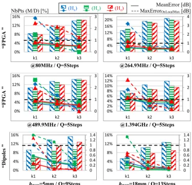
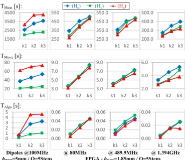
6 presents the comparison between full sampling at d=0.5mm and optimized sampling using adaptive algorithm for the three magnetic field components (Hx, Hy and Hz) at three
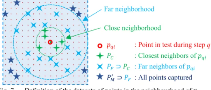
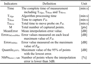
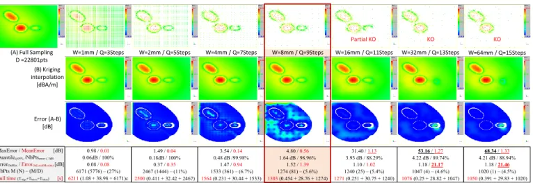
The orientation retained in this paper is to reduce the number of measurement points by capturing only points which bring the most information selected by a
