A compound unit method for incorporating
ordered compounds into lattice models of alloys
The MIT Faculty has made this article openly available. Please share
how this access benefits you. Your story matters.
Citation Kalidindi, Arvind R. and Christopher A. Schuh. “A Compound Unit
Method for Incorporating Ordered Compounds into Lattice Models of Alloys.” Computational Materials Science 118 (June 2016): 172–179 © 2016 Elsevier B.V.
As Published https://doi.org/10.1016/j.commatsci.2016.02.039
Publisher Elsevier
Version Author's final manuscript
Citable link http://hdl.handle.net/1721.1/116381
Terms of Use Creative Commons Attribution-NonCommercial-NoDerivs License
1
A compound unit method for incorporating ordered compounds into lattice models of alloys
Arvind R. Kalidindia, Christopher A. Schuha,*
a Department of Materials Science and Engineering, Massachusetts Institute of Technology, Cambridge, MA 02139, USA.
*Corresponding author at: [email protected].
2
Abstract
Lattice models can be a basic tool for alloy design, due to their ability to capture the most important thermodynamic and kinetic phenomena of a wide-range of alloys at a low computational cost. However, in order to correctly treat ordered precipitates at off-stoichiometric compositions requires multi-body potentials, and these can be challenging to calibrate to known alloy behaviors. Here we introduce a simple means of capturing the multi-body terms needed to treat ordered compounds in a lattice model based on defining “compound units”. This approach is particularly designed for, and easily calibrated in, cases where the structure and formation energy of equilibrium compounds are already known. This is accomplished by defining a compound unit that derives its energy from the formation energy of the compound as an a priori input. The method is illustrated for a binary alloy with D03 and B2 stable compounds.
Highlights
• A method for incorporating known ordered compounds into a lattice model is proposed. • The method maintains the simplicity and broad applicability of the pairwise model. • A compound unit is used to capture the compound’s structure and formation energy. • Monte Carlo simulations show that this method produces proper two-phase behavior.
Graphical Abstract
5 at.% 10 at.% 15 at.% 20 at.% 25 at.%
5 at.% 10 at.% 15 at.% 20 at.% 25 at.%
Pairwise Model at 0K
3
1. Introduction
Lattice models provide a convenient framework for studying the evolution and stability of alloy microstructures [1-15]. These models typically focus on the mesoscale behavior of the system, describing the state of the alloy on a fixed lattice, with an interatomic potential that expresses the relative preference for different arrangements of species on the lattice. A pairwise potential is often used because of its simplicity for implementation and easy adaptability for conducting rapid surveys across many material systems [1-4,16-20]. The pairwise potential for a binary alloy can generally be written as:
𝐻𝐻 = � 𝐽𝐽(𝑘𝑘)(1 − δ 𝜎𝜎i𝜎𝜎j) {i,j}
(1)
The summation is conducted over all pairs of lattice sites, where σi = 1 for a solvent atom and -1 for a solute atom located at lattice site i, and δis a Kronecker delta, which is 1 for like bonds (solvent-solvent (AA) and solute-solute (BB)) and 0 for solute-solvent bonds (AB). 𝐽𝐽(𝑘𝑘) is the pairwise interaction parameter describing the difference in pairwise bond energy, E, between like and unlike pairs at a neighbor distance of k: 𝐽𝐽(𝑘𝑘) = 𝐸𝐸𝐴𝐴𝐴𝐴(𝑘𝑘)−(𝐸𝐸𝐴𝐴𝐴𝐴
(𝑘𝑘)+𝐸𝐸 𝐵𝐵𝐵𝐵(𝑘𝑘))
2 . By varying 𝐽𝐽(𝑘𝑘) many different alloy systems can be represented using this general description.
When considering only nearest-neighbor interactions (k = 1), a shortcoming of the pairwise potential for modeling negative enthalpy of mixing alloys becomes apparent. For a positive enthalpy of mixing alloy (J(1) > 0), the internal energy can be minimized by forming separate solute and solvent phases, and thus at 0K the thermodynamic equilibrium state consists of two phases that are immiscible in one another. In a negative enthalpy of mixing alloy (J(1) < 0), thermodynamically it is expected that an ordered compound will be formed to minimize internal energy such that at 0K the equilibrium state again consists of two phases that satisfy the zero entropy requirement of the third law of thermodynamics. The pairwise model does not produce this result for negative enthalpy of mixing alloys, instead predicting a disordered alloy state (solid solution) to be thermodynamically stable. Moreover, this limitation is inherent to the pairwise potential, and thus exists regardless of whether the equilibrium state is determined via the cluster variation method [7-9] or a Monte Carlo simulation [1,6].
4
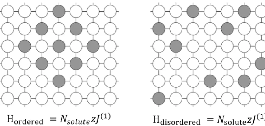
This anomalous behavior can be attributed to the insufficient description of ordering using a pairwise potential, which is illustrated in Figure 1 for the case of a two-dimensional square lattice. In this schematic, one system contains an ordered compound, while the second system is disordered. According to Equation 1, both of these systems have the same internal energy since each solute is bonded to only solvent atoms in both situations, which is also the lowest energy state possible for the system. Because the second system is disordered, it has higher entropy and is therefore found to be stable at all finite temperatures.
The repercussions of this shortcoming are not limited to the 0K equilibrium. In a pairwise model, ordering only occurs when the solute concentration is large enough to impose a geometrical constraint, e.g. when a disordered phase requires forming solute-solute bonds at an energetic cost. For example, the nearest neighbor model exhibits an equiatomic compound in the 2D square lattice because at this stoichiometry the only way to attain all solute-solvent bonds is to form an ordered phase. While the above discussion mainly focuses on the nearest neighbor model to simplify the explanation, this behavior is expected to be present at absolute zero for any pairwise model with negative interaction parameters [1,7-9]. The inability to capture accurate ordering tendencies limits the usefulness of such a description for designing alloys, where it is often desirable to study the
Figure 1. The schematic shows two solute arrangements, ordered (on left) and disordered (on right). The internal energies calculated by Equation 1 in the nearest neighbor approximation are equivalent in both cases, making ordered phases unstable at off-stoichiometric concentrations (Nsolute is the number of solutes and z is the coordination number).
5
precipitation of an ordered compound at off-stoichiometric compositions, and in systems where ordering has additional energetic implications beyond merely the geometric ones.
The standard route to better incorporate an alloy’s ordering tendency is to include the interactions of multiple atoms, and thus allow ordered states to access a lower internal energy [21-25]. A general formulation for introducing the multi-body terms can be written as:
𝐻𝐻 = � 𝐽𝐽𝑖𝑖𝜎𝜎𝑖𝑖 𝑠𝑠𝑖𝑖𝑠𝑠𝑠𝑠𝑠𝑠𝑠𝑠𝑠𝑠 + � 𝐽𝐽𝑖𝑖𝑖𝑖𝜎𝜎𝑖𝑖𝜎𝜎𝑖𝑖 𝑝𝑝𝑝𝑝𝑖𝑖𝑝𝑝𝑠𝑠 + � 𝐽𝐽𝑖𝑖𝑖𝑖𝑘𝑘𝜎𝜎𝑖𝑖𝜎𝜎𝑖𝑖𝜎𝜎𝑘𝑘 𝑠𝑠𝑝𝑝𝑖𝑖𝑝𝑝𝑠𝑠𝑠𝑠𝑠𝑠𝑠𝑠 … (2)
where the J terms are now called effective cluster interactions. A typical procedure for predicting the bulk phase diagrams of different alloy systems is to calculate compound formation energies using density functional theory, and then using these to infer reasonable effective cluster interactions (called the Structure Inversion Method or Connolly-Williams method [21]). Generally, this requires consideration of 30-50 possible ordered compounds in order to determine a set of 10-100 interaction parameters that are deemed the most important for the interaction potential.
This method of including multi-body terms has been useful for developing bulk phase diagrams of alloys [26-29]. Increasingly, however, lattice models are being extended outside of classical bulk thermodynamic behavior, for instance to study the effects of interfaces [16-18,31-35]. In such cases, while using a cluster expansion to define the interatomic potential may still be feasible, it is not optimal because (i) the stability of compounds in bulk systems is already known [30], and thus “predicting” the stable compounds through simulation is unnecessary and (ii) the multi-body terms are calculated for each alloy system and thus too specific to probe a large number of alloy combinations and often not easily extendable to non-bulk environments. In some of our group’s work on nanostructured alloys we have found a need for a lattice-based method that can be rapidly calibrated to known bulk thermodynamics and then used to explore, e.g., driven processing through ballistic mixing [34] or deposition [35], or simply to explore the space of accessible structures in nanostructured systems [18,36-38]. It is our purpose in this paper to present such a method that overcomes the limitations of the pairwise model in describing negative enthalpy of mixing systems, specifically for cases where the structure and formation energy of equilibrium compounds are already known, and a full cluster expansion would be redundant.
6
2. Compound Unit Model
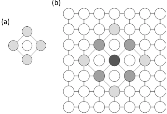
In order to permit stable compounds in a pairwise model, a distinction has to be drawn between solute-solvent bonds in a solid solution and those in an ordered phase. Rather than add multiple higher order terms as in Equation 2, we directly include an ordered compound with known structure and formation energy into a nearest-neighbor pairwise formalism by identifying its structure through a “compound unit”. A compound unit is defined here as a repeating group of atoms from which the entire superstructure of the compound can be formed. For example, we may define the compound unit shown in Figure 2a to identify the compound shown in Figure 1. Many potential compound units may be defined – the selection of appropriate compound units is discussed in Section 2.1, but the key feature of the unit is that when it appears in the structure, it will be assigned a lower enthalpy than what the pairwise potential would return, and which is related to the compound formation energy. If a compound unit, α, is found in the lattice, the energy is instead calculated based on an additional interaction parameter for the compound, Jα, which can be expressed as:
𝐽𝐽α = 𝑁𝑁α𝛥𝛥𝐻𝐻𝑓𝑓𝑓𝑓𝑝𝑝𝑓𝑓− � 𝐽𝐽(𝑘𝑘)(1 − δ𝜎𝜎i𝜎𝜎j) {𝑖𝑖,𝑖𝑖}𝑖𝑖𝑖𝑖 α
fα (3)
where Δ𝐻𝐻𝑓𝑓𝑓𝑓𝑝𝑝𝑓𝑓 is the formation energy of the compound per atom, which is multiplied by the effective number of atoms in the compound unit, Nα. The second term in this expression removes the pairwise contribution to energy of the compound unit (fa is the fraction of the bond that is contained in a particular compound unit), so that its energy is solely described by the formation energy of the compound. For a compound to be enthalpically preferable to a solid solution, Jα should be negative to account for the additional enthalpic benefit of ordering.
The pairwise potential is appended to include an enthalpic benefit for compounds: 𝐻𝐻 = � 𝐽𝐽(𝑘𝑘)(1 − δ 𝜎𝜎i𝜎𝜎j) {𝑖𝑖,𝑖𝑖} + � 𝐽𝐽α𝑀𝑀α {α} (4)
The contribution of compound unit energies is calculated by counting the number of units of a particular compound in the system, Mα, and applying the enthalpic benefit, Jα, for each compound unit being considered. This similarly applies to calculating the energy of an individual atom: the energy is calculated entirely from pairwise interactions if none of the environment around the atom resembles a compound unit, but if the atom is part of a compound unit then that portion of its
7
energy is replaced by the compound unit energy. This is illustrated in Figure 2b, where the interior atom of the compound has its complete energy described by the compound unit energy, as opposed to atoms on the edges and corners which respectively have one-half and one-quarter of their energies described by the compound unit energy, with the remainder calculated from pairwise bonds.
2.1 Selection of Compound Units
Subdividing the environment around an atom into an appropriate compound unit and counting these during a simulation is an important aspect of our method. To illustrate the selection of a compound unit, the D03 (25 at.% stoichiometry) and B2 (50 at.% stoichiometry) compounds in the body-centered cubic system are considered.
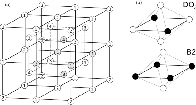
The superstructure of these compounds is conveniently represented by describing the occupancy of the four interpenetrating face-centered cubic sublattices in a body-centered cubic structure, as shown in Figure 3a. The D03 compound exists when one of the face-centered cubic sublattices is occupied by solute, and the other three are occupied by solvent, thus fulfilling the 25 at.% stoichiometry. The B2 compound exists when two non-adjacent face-centered cubic sublattices are occupied by solutes, and solvent atoms occupy the other two. Convenient compound units for each of these two compounds are shown in Figure 3b, with example corresponding lattice
(a)
(b)
Figure 2. (a) Shows a possible definition of a compound unit for the ordered compound pictured in Figure 1, where dark atoms are solute. (b) Shows a schematic of how the energy of an atom is calculated in the compound unit model, where darker atoms have a larger compound unit contribution to their energy.
8
sites shaded in Figure 3a. The compound units are effectively solute-centric as they can be considered to divide the environment around a solute atom into 1/12th partitions (N𝑖𝑖,𝛼𝛼𝑠𝑠𝑓𝑓𝑠𝑠𝑝𝑝𝑠𝑠 = 12), where each unit consists of two first nearest neighbors, two second nearest neighbors, and one of the twelve third nearest neighbors of the solute. The necessary size of the compound unit is determined based on the compound superstructure, where in this case third nearest neighbors were required for the D03 compound since this is the neighbor distance of solute in this compound.
Part of the consideration in determining a suitable compound unit is the ease with which the simulation method will be able to find the equilibrium state. For example, one choice of a compound unit would be to consider the full environment around a central atom out to third nearest neighbors in all directions. In this scenario, no energetic benefit would be applied until all of the second and third nearest neighbors of the compound fell into place. Since this is not a common occurrence, a Monte Carlo simulation is more prone to being trapped in a metastable solid solution due to the kinematic difficulty of forming a compound unit, even if it would decrease the free energy to form compound units. Thus, choosing a compound unit that is more readily formed
(a) (b)
Figure 3. (a) A schematic of the compound superstructure for D03 and B2 compounds in body-centered cubic binary alloys, with numbers signifying different interpenetrating FCC sublattices. Convenient compound units for D03 and B2 are shown in (b), with solute in black. Shaded atoms in (a) illustrate the compound unit within the superstructure.
1 1 1 1 1 1 1 1 1 1 1 1 1 2 2 2 2 2 2 2 2 2 2 2 2 2 2 3 3 3 3 4 4 4 4
DO
3B2
9
stochastically by Monte Carlo events, accomplished in this case by defining a compound unit that includes only the one necessary third nearest neighbor, is desirable to achieve ergodic sampling and find the true thermodynamic equilibrium state.
From the perspective of a pairwise bonding scheme, the inclusion of these compound unit energies is a targeted way to incorporate the formation energies of known compounds to replicate bulk thermodynamic behavior. On the other hand, this can also be viewed as a simplification of the multi-body potential in Equation 2. The value of the structural inversion method for incorporating ordered compounds is that the potential is trained on a set of ordered compounds constructed by density functional theory, and thus consequent simulations with this potential can reveal which compounds are found at equilibrium. In our present method, by contrast, we assume knowledge of the relevant equilibrium ordered compounds and thus rather than performing a full cluster expansion this method includes a select few energy terms to produce proper ordering behavior while maintaining the convenience of a pairwise description for the remainder of the physics in the model.
3. Case Study
The thermodynamic equilibrium of an alloy described by the compound unit model was determined using a lattice-based Monte Carlo simulation. A lattice was constructed with a fixed composition and a random distribution of solutes. In each Monte Carlo event, a random solute and solvent atom from anywhere within the lattice were swapped to create a new configuration in the phase space, and this transition was accepted according to the Metropolis algorithm (the transition was always accepted if the energy of the new configuration was lower, and was accepted with a probability, 𝑒𝑒−𝛥𝛥𝛥𝛥k𝑇𝑇, if the new energy was larger by ΔE, where k is the Boltzmann constant and T is the temperature). While the ordering term in Equation 4 was not written as a sum over lattice sites, the ordering contribution to the change in energy from a swap was determined quickly by counting the number of compound units containing the swapped atoms that were created or disrupted by the swap and multiplying by the appropriate compound interaction parameters.
Monte Carlo simulations were conducted for a binary, body-centered cubic alloy with stable D03 and B2 compounds. Two sets of calculations were conducted using this Monte Carlo
10
setup. In the control simulations, the system was described purely using pairwise bond energies, considering up to second nearest neighbor bonds with interaction parameters of J(1) = -32.4 meV/bond and J(2) = -16.2 meV/bond, which are known to produce stable D03 and B2 compounds [39]. In the second set, the compound unit model was used, considering nearest neighbor pairwise bonds, still with an interaction parameter of J(1) = –32.4 meV/bond, and with compound unit interaction parameters, JD03 = -16.1 meV/unit and JB2 = -10.3 meV/unit, for the compound units in Figure 3b. These compound unit energies were selected in order to produce D03 and B2 compounds with the same formation energy as in the pairwise model, where the formation energies of the two compounds are -89 meV/atom and -145 meV/atom, respectively. The values of the interaction energies were verified by constructing each compound at stoichiometry and ensuring that the total energy of the system was equal to the formation energy of the ordered compound. A three-dimensionally periodic simulation of 64,000 atoms at a temperature of 2,500 K and was equilibrated for 50,000 Monte Carlo steps (1 step consists of 64,000 swap attempts). Subsequently the temperature is repeatedly lowered by 50 K and equilibrated for 10,000 Monte Carlo steps at each new temperature to determine the equilibrium state down to 0 K. Since at each temperature the equilibrated structure from the previous, higher temperature state is used as the initial state, this method produces reasonable predictions of low temperature equilibrium structures. The simulations were conducted for solute concentrations ranging from 1 to 50 at.%, with additional simulations conducted in increments of 10K within 100K of the critical temperature to attain a higher resolution.
3.1 Simulations at 0K
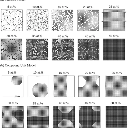
The pairwise potential cannot accurately capture ordering in two-phase fields, and the addition of a compound unit term is a purposeful mend to this problem. Figure 4 shows the solute atoms in the (100) plane of equilibrated structures with and without the compound unit term at different compositions. At the 25 at.% and 50 at.% stoichiometries, the D03 and B2 compounds are the equilibrium phases in both cases. However, deficiencies in the pairwise model are already evident; in Figure 4a at 25 at.%, two antiphase boundaries are observed and indicated with arrows. These defects should not be present at equilibrium in a single phase compound, and appear because they are trapped in this simulation. This difficulty in achieving long range order is a common problem when studying compounds in the Ising model with a pairwise potential [1,40]. However,
11
in the compound unit approach, antiphase boundaries are more energetic and not easily trapped, which yields the correct equilibrium microstructure as shown in Figure 4b at 25 at.%.
The more serious deficiencies of the pairwise model appear at off-stoichiometric compositions, where faceted precipitates in a two-phase equilibrium are thermodynamically expected at 0K. The equilibrated structures in Figure 4a have non-zero entropies, as evidenced by the large degeneracy of the equilibrium states, which is attributed to the phenomena explained in Figure 1. At the stoichiometric composition, the equilibrium is a single-phase compound that is forced to form by geometry, and it does not require a non-zero interfacial energy. At slightly
off-(a) Pairwise Model
(b) Compound Unit Model 5 at.% 10 at.%
40 at.%
30 at.% 45 at.% 50 at.%
15 at.% 20 at.% 25 at.%
35 at.%
Figure 4. Equilibrium states computed at 0K via a Monte Carlo simulation under (a) the pairwise model and (b) the compound unit model. Only solute atoms are shown in the image, on a single (100) plane of the simulation cell.
12
stoichiometric compositions, local ordering is observed via this same constraint, but a single consolidated phase is not preferred energetically because there is no energetic penalty associated with forming an interface between the compound and solvent atoms. At low concentrations, this leads to a solid solution as there are many sites where solute can reside and still achieve ideal first and second nearest neighbor coordination.
In contrast, and shown in Figure 4b, the compound unit model produces equilibrium structures with the expected two-phase equilibrium at off-stoichiometric compositions at 0K. Firstly, the addition of compound units fixes the energetics such that the ground state of the alloy is now two, separated phases at 0K. Secondly, this formulation makes it convenient for Monte Carlo simulations to find the correct equilibrium state even at low temperatures since each atom at the interface possesses an interfacial energy; the system thus correctly coarsens into a single precipitate, and can avoid producing anti-phase boundaries.
3.2 Order-Disorder transitions
The more realistic occurrence of ordering in the compound unit model not only satisfies the third law of thermodynamics, but also captures reasonable order-disorder behavior, which is not present at low compositions in the pairwise model.
A natural set of order parameters arises from the compound unit formulation because each solute atom in the system has a certain number of compound units of which it is a member. For example, a solute atom in solution would not be a part of any compound units, a solute atom in the compound phase should have a full coordination of compound units (in our BCC example, this is 12), and any level of coordination in between corresponds to different degrees of order (for instance at phase boundaries or local ordering in solution). Formally, this set of short-range order parameters can be written as:
𝜂𝜂𝑓𝑓α =N 1
solute � 𝛿𝛿𝑁𝑁j α,𝑓𝑓 j
for 𝑚𝑚 = 0 to N𝑖𝑖,α𝑠𝑠𝑓𝑓𝑠𝑠𝑝𝑝𝑠𝑠 (5)
where 𝜂𝜂𝑓𝑓α is the order parameter describing solute atoms that are part of m compound units of phase α. Here, the summation runs over only lattice sites containing a solute atom. 𝑁𝑁jα is the number of compound units of phase α around the solute atom at site ‘j’, and Nsolute is the number of solutes in the system. This general set of m order parameters could be particularly useful for
13
describing how the ordering changes through the inclusion of non-bulk behavior, for instance due to the presence of grain boundaries and surfaces, which is a topic of some of our future work. For the purposes of the present study, we limit our attention to 𝜂𝜂12α for both the D03 and B2 compounds, which signifies the fraction of solutes in a completely ordered local state. The 𝜂𝜂12α order parameter in particular is chosen as it behaves most like a long-range order parameter; it can only have a value close to unity if a large single-phase region exists in the material.
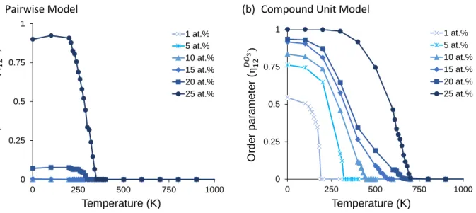
Figure 5 shows the value of the order parameter, 𝜂𝜂12D03, as a function of temperature for different compositions at and below 25 at.% for both the pairwise and compound unit models. In the pairwise model (Figure 5a), the order parameter is only markedly greater than zero for solute concentrations above 15 at.%, which matches what was observed in the equilibrium microstructures in Figure 4a where larger clusters of the D03 compound are found starting at 20 at.%. In contrast, the compound unit model (Figure 5b) has non-zero values for the order parameter at 0K for all compositions below 25 at.%, though the value of the order parameter at 0K only reaches unity at the stoichiometry of the compound, where the system is in a single-phase, fully ordered state (it does not reach unity in the pairwise model due to the presence of anti-phase boundaries). When the ordered phase is in equilibrium with a second phase, the order parameter will be less than unity as some of the solute atoms reside at the interface and are not fully ordered.
(a) Pairwise Model (b) Compound Unit Model
Figure 5. The D03 order parameter with respect to system temperature at compositions {1,5,10,15,20,25} at.% for (a) the pairwise model and (b) the compound unit model.
Temperature (K) O rder par am et er ( 0 0.25 0.5 0.75 1 0 250 500 750 1000 1 at.% 5 at.% 10 at.% 15 at.% 20 at.% 25 at.% O rder par am et er ( Temperature (K) 0 0.25 0.5 0.75 1 0 250 500 750 1000 1 at.% 5 at.% 10 at.% 15 at.% 20 at.% 25 at.%
14
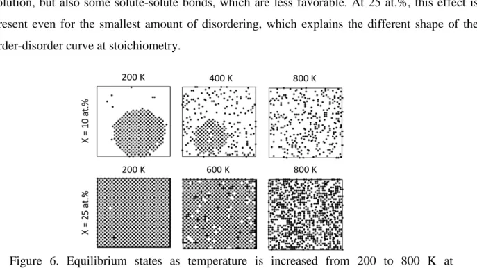
In all cases in the compound unit model, as the temperature increases, the ordering decreases, with a sharp drop approaching the phase transition. Figure 6 shows the equilibrium states at compositions of 10 and 25 at.% during this disordering processes. As expected, at non-zero temperatures, each phase exhibits some solubility of the second phase, and as the temperature increases the amount of the ordered phase decreases until it disappears above the phase transition temperature. Interestingly, as the composition increases from 10-20 at.%, the drop in the order parameter (Figure 5b) becomes less sharp, and approaches an order parameter of zero more gradually. Because 𝜂𝜂12α is not a true long range order parameter, the shape of this curve at the transition does not characterize the transition as being either first or second order. Instead, this seems to be due to compositions closer to stoichiometry being constrained in their ability to disorder – in order for it to disorder fully, it requires not only forming solute-solvent bonds in solution, but also some solute-solute bonds, which are less favorable. At 25 at.%, this effect is present even for the smallest amount of disordering, which explains the different shape of the order-disorder curve at stoichiometry.
3.3 Phase Diagrams
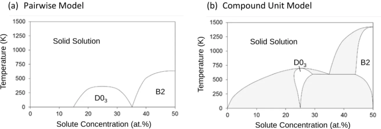
The 𝜂𝜂12D03 and 𝜂𝜂12B2 order parameters were used to construct phase diagrams of both the pairwise and compound unit models, shown in Figure 7, with two-phase regions shaded. The critical temperature of a phase transition was determined by identifying the temperature at which
800 K X = 10 a t.% X = 25 a t.% 400 K 200 K 600 K 200 K 800 K
Figure 6. Equilibrium states as temperature is increased from 200 to 800 K at compositions of 10 and 25 at.%. Only solute atoms are shown in the image, with atoms
15
an order parameter exhibits a discontinuity in slope, and was corroborated with visual evidence of phase changes in the equilibrium microstructures.
There are a few important differences between the two phase diagrams. At low concentrations, the compound unit model produces the expected two-phase equilibrium with the A-rich solid solution phase. The lack of this two-phase region in the pairwise model was the principle reason for incorporating compound units, and the phase diagram demonstrates that this approach fixes the anomalous thermodynamic behavior in the pairwise model. Similarly, there is a two-phase region that exists between the D03 and B2 phases in the compound unit model that is absent in the pairwise model. Other pairwise models simulating a system with D03 and B2 compounds produce a second order phase transition between the D03 and B2 phases [7,8], which would also violate the third law of thermodynamics, as one or both phases would have to have a non-zero solubility at 0K. Thus, the presence of this two-phase region also seems to be an improvement made by the inclusion of compound unit energies.
The critical temperature for disordering is also lower for the compounds in the pairwise model than in the compound unit model, since only geometric considerations lead to ordering, whereas in the compound unit model both geometric and chemical interactions favor the ordered phases. The adherence of the phase diagram produced by the compound unit model to basic thermodynamic principles provides confidence that this approach is a viable alternative to a full
(a) Pairwise Model (b) Compound Unit Model
Figure 7. Phase diagrams in (a) the pairwise model and (b) the compound unit model calculated via Monte Carlo. Phase transitions are denoted with solid lines, and two-phase regions are shaded.
T em per at ur e ( K )
Solute Concentration (at.%)
D03 B2 Solid Solution T em per at ur e ( K )
Solute Concentration (at.%) Solid Solution
B2
16
multi-body expansion for incorporating bulk ordering thermodynamics into lattice models of alloys.
3.4 Application to Non-Bulk Systems
The compound unit method’s main benefit is its ability to account for an alloy’s ordering tendency without adding substantial complexity to the model. This is particularly useful when simulating non-bulk systems, where the added complexity of the system can be compounded by a complicated interatomic potential. To demonstrate such a scenario, we added an interface into the Monte Carlo simulations, and described the tendency for solute segregation to the interface using an interaction parameter, 𝐽𝐽int, to prescribe the energies of bonds across the interface: 𝐽𝐽int = 𝐸𝐸ABint− (𝐸𝐸AAint+𝐸𝐸BBint)
2 , where 𝐸𝐸AAint = 𝐸𝐸BBint. Segregation of solute to the interface is favored when 𝐽𝐽int < 𝐽𝐽(1), because under this condition forming solute-solvent bonds at the interface reduces the energy of the system more than forming solute-solvent bonds in the bulk. The enthalpy of segregation can be related to the interaction parameters as Δ𝐻𝐻seg = 4�𝐽𝐽(1)− 𝐽𝐽int�, with ΔHseg having a positive value when grain boundary segregation is favored and the coefficient accounts for the number of bonds across the interface for an atom located at the interface .
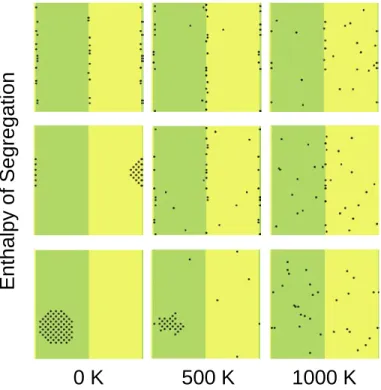
Simulations were conducted using the bulk energies from the single crystal studies for different positive enthalpies of segregation to the interface (Figure 8). Three distinct regimes are found. At low enthalpies of segregation, a compound forms at low temperatures and disorders into a solid solution. At high enthalpies of segregation, segregation to the interfaces is the lowest energy state, and disorders into a solid solution. At intermediate enthalpies of segregation, there are two transitions: first the compound disorders into an interface-segregated state, which then disorders into a solid solution.
17
With the inclusion of the interface, the solute elements now have three basic options: either dissolve into a solid solution, form into an ordered compound, or segregate to the interface. The competition between these options depends on the bond energies, temperature, composition, and interfacial area. Establishing the relationship between these inputs and the equilibrium microstructure is generally challenging, and conventional methods such as the structural inversion method do not provide a simple means of tuning the formation energy of the compound, enthalpy of mixing, or enthalpy of interfacial segregation to explore this alloy design space. Using the compound unit model, the energy inputs can be readily tuned and related to bulk thermodynamic properties, and the resulting thermodynamic behaviors can be explored.
Figure 8. Equilibrium states for a system with an interface for different enthalpies of segregation to the interface (50, 250, and 300 meV/atom from bottom to top) and at different temperatures. All simulations were conducted with 1 at.% solute and with periodic boundary conditions (so the left and right sides of the simulation cell plane are interfaces as well).
E
nt
hal
py
of
S
egr
egat
ion
1000 K
500 K
0 K
18
4. Conclusions
Lattice models are a convenient tool for developing a phenomenological understanding of the thermodynamics and kinetics of alloys, and the pairwise potential has long been useful for rapid surveys across the alloy design space. However, the pairwise potential is not able to capture compound formation in a thermodynamically consistent way, and this has limited the use of lattice models and in particular the pairwise potential lattice model for studying alloys where ordering is important, such as in negative enthalpy of mixing systems. The compound unit method is a simple patch to the pairwise model that for the most part maintains the simplicity of the pairwise description, but adds an energetic benefit when the local environment around an atom resembles a stable compound in the system. This model is designed to be useful for systems where the bulk thermodynamics, and thus the structure and formation energy of stable compounds, are already known, and the goal is to study non-bulk behavior, such as the influence of defects, interfaces, and processing conditions on a material’s equilibrium structure.
Acknowledgements—This work was supported by the U.S. Army Research Office under grant
W911NF-14-1-0539. ARK would like to acknowledge the support of a National Science Foundation Graduate Research Fellowship.
19
References
[1] K. Binder, D.P. Lindau, Phase diagrams and critical behavior in Ising square lattices with nearest- and next-nearest-neighbor interactions, Phys. Rev. B 21 (1980) 1941.
[2] K. Binder, Ordering of the face-centered-cubic lattice with nearest-neighbor interaction, Phys. Rev. Lett. 45 (1980) 811-814.
[3] K. Binder, J.L. Lebowitz, M.K. Phani, M.H. Kalos, Monte Carlo study of the phase diagrams of binary alloys with face centered cubic lattice structure, Acta Metall. 29 (1981) 1655-1665. [4] M.K. Phani, J.L. Lebowitz, M.H. Kalos, C.C. Tsai, Monte Carlo study of an ordering alloy on an fcc lattice, Phys. Rev. Lett. 42 (1979) 577-580.
[5] J.M. Sanchez, D. de Fontaine, Ising model phase-diagram calculations in the fcc lattice with first- and second-neighbor interactions, Phys. Rev. B 25 (1982) 1759.
[6] L. Guttman, Monte Carlo computations on the Ising model: The body-centered cubic lattice, J. Chem. Phys. 34 (1961) 1024-1036.
[7] H. Ackermann, G. Inden, R. Kikuchi, Tetrahedron approximation of the cluster variation method for b.c.c. alloys. Acta Metall. 37 (1989) 1-7.
[8] C. Colinet, G.Inden, R. Kikuchi, CVM calculation of the phase diagram of b.c.c. Fe-Co-Al. Acta Metalll. 41 (1993) 1109-1118.
[9] L.T.F. Eleno, C.G. Schon, CVM calculation of the b.c.c. Co-Cr-Al phase diagram. Calphad 27 (2003) 335-342.
[10] G. Ceder, A derivation of the Ising model for the computation of phase diagrams, Comp. Mat. Sci. 1 (1993) 144-150.
[11] B. Sadigh, P. Erhart, A. Stukowski, A. Caro, E. Martinez, L. Zepeda-Ruiz, Scalable parallel Monte Carlo algorithm for atomistic simulations of precipitation in alloys, Phys. Rev. B 85 (2012) 184203.
[12] K. Yaldram, K. Binder, Monte Carlo simulation of phase separation and clustering in the ABV model, J. Stat. Phys. 62 (1991) 161-175.
20
[13] Z. Mao, C.K. Sudbrack, K.E. Yoon, G. Martin, D.N. Seidman, The mechanism of
morphogenesis in a phase-separating concentrated multicomponent alloy, Nature Mat. 6 (2007) 210-216.
[14] P.S. Sahini, D.J. Srolovitz, G.S. Grest, M.P. Anderson, S.A. Safran, Kinetics of ordering in two dimensions. II. Quenched systems, Phys. Rev. B 28 (1983) 2705.
[15] E.A. Holm, C.C. Battaile, The computer simulation of microstructural evolution, JOM, 53 (2001) 20-23.
[16] P. Bellon, R.S. Averback, Nonequilibrium roughening of interfaces in crystals under shear: Application to ball milling, Phys. Rev. Lett. 74 (1995) 1819-1822.
[17] B. Yang, M. Asta, O.N. Mryasov, T.J. Klemmer, R.W. Chantrell, The nature of A1-L10 ordering transitions in alloy nanoparticles: A Monte Carlo study, Acta Mater. 54 (2006) 4201-4211.
[18] T. Chookajorn, C.A. Schuh, Thermodynamics of stable nanocrystalline alloys: A Monte Carlo analysis, Phys. Rev. B (2014) 064102.
[19] J. Erlebacher, M.J. Aziz, A. Karma, N. Dimitrov, K. Sieradzki, Evolution of nanoporosity in dealloying, Nature 410 (2001) 450-453.
[20] F. Lanzini, R. Romero, Thermodynamics of atomic ordering in Cu-Zn-Al: A Monte Carlo study, Comp. Mat. Sci. 96 (2015) 20-27.
[21] J.W. Connolly, A.R. Williams, Density-functional theory applied to phase transformations in transition metal alloys, Phys. Rev. B 27 (1983) 5169.
[22] J.M. Sanchez, F. Ducastelle, D. Gratias, Generalized cluster description of multicomponent systems, Physica A 128 (1984) 334-350.
[23] M. Asta, C. Wolverton, D. de Fontaine, H. Dreyssé, Effective cluster interactions from cluster-variation formalism. I., Phys. Rev. B 44 (1991) 4907.
[24] D.B. Laks, L.G. Ferreira, S. Froyen, A. Zunger, Efficient cluster expansion for substitutional systems, Phys. Rev. B 46 (1992) 12587.
21
[25] A. van de Walle, G. Ceder, Automating first-principles phase diagram calculations, J. Phase Equilib. 23 (2002) 348-359.
[26] S.H. Wei, L.G. Ferreira, A. Zunger, First-principles calculation of temperature-composition phase diagrams of semiconductor alloys, Phys. Rev. B 41 (1990) 8240.
[27] K. Terakura, T. Oguchi, T. Mohri, K. Watanabe, Electronic theory of the alloy phase stability of Cu-Ag, Cu-Au, Ag-Au. Phys. Rev. B 35 (1987) 2169.
[28] V. Ozolins, C. Wolverton, A. Zunger, Cu-Au, Ag-Au, Cu-Ag, and Ni-Au intermetallics: First-principles study of temperature-composition phase diagrams and structures, Phys. Rev. B 57 (1998) 6427.
[29] M. Asta, R. McCormack, D.D de Fontaine, Theoretical study of alloy phase stability in the Cd-Mg system, Phys. Rev. B 48 (1993) 748.
[30] S. Curtarolo, W. Setyawan, S. Wang, J. Xue, K. Yang, et. al., AFLOWLIB.ORG: A distributed materials properties repository from high-throughput ab initio calculations, Comp. Mat. Sci. 58 (2012) 227-235.
[31] W. Schweika, D.P Landau, K. Binder, Surinduced ordering and disordering in face-centered-cubic alloys: A Monte Carlo study, Phys, Rev. B 53 (1996) 8937.
[32] M. Müller, K. Albe, Lattice Monte Carlo simulations of FePt nanoparticles: Influence of size, composition, and surface segregation on order-disorder phenomena, Phys. Rev. B 72 (2005) 094203.
[33] R.V. Chepulskii, W.H. Butler, Temperature and particle-size dependence of the equilibrium order parameter of FePt alloys, Phys. Rev. B 72 (2005) 134205.
[34] Z.C. Cordero, C.A. Schuh, Phase strength effects on chemical mixing in extensively deformed alloys, Acta Mater. 29 (2015) 123-136.
[35] S. Ruan, C.A. Schuh, Kinetic Monte Carlo simulations of nanocrystalline film deposition, J. Appl. Phys. 107 (2010) 073512.
[36] T. Chookajorn, C.A. Schuh, Nanoscale segregation behavior and high-temperature stability of nanocrystalline W–20at.% Ti, Acta Mater. 73 (2014) 128-138.
22
[37] T. Chookajorn, M. Park, C.A. Schuh, Duplex nanocrystalline alloys: Entropic nanostructure stabilization and a case study on W–Cr, J. Mater. Res. 30 (2015) 151-163.
[38] A.R. Kalidindi, T. Chookajorn, C.A. Schuh, Nanocrystalline materials at equilibrium: A thermodynamic review, JOM, 67 (2015) 2834-2843.
[39] S.M. Allen, J.W. Cahn, Ground state structures in ordered binary alloys with second neighbor interactions, Acta. Metall. 20 (1972) 423-433.
[40] U. Gahn, Ordering in face-centered cubic binary crystals confined to nearest-neighbour interactions–Monte Carlo calculations, J. Phys. Chem. Solids 47 (1986) 1153-1169.