Productive Capacity of Biodiversity: Crop Diversity and Permanent Grasslands in Northwestern France

HAL Id: hal-02925099

https://hal.inrae.fr/hal-02925099

Submitted on 26 Feb 2021

HAL is a multi-disciplinary open access archive for the deposit and dissemination of sci-entific research documents, whether they are pub-lished or not. The documents may come from teaching and research institutions in France or abroad, or from public or private research centers.

L’archive ouverte pluridisciplinaire HAL, est destinée au dépôt et à la diffusion de documents scientifiques de niveau recherche, publiés ou non, émanant des établissements d’enseignement et de recherche français ou étrangers, des laboratoires publics ou privés.

Distributed under a Creative Commons Attribution - NonCommercial - ShareAlike| 4.0 International License

Productive Capacity of Biodiversity: Crop Diversity and

Permanent Grasslands in Northwestern France

François Bareille, Pierre Dupraz

To cite this version:

François Bareille, Pierre Dupraz. Productive Capacity of Biodiversity: Crop Diversity and Permanent Grasslands in Northwestern France. Environmental and Resource Economics, Springer, 2020, 77 (2), pp.365-399. �10.1007/s10640-020-00499-w�. �hal-02925099�

1

Productive capacity of biodiversity: crop diversity and permanent grasslands in

1

northwestern France

2 3

François Bareille a*, Pierre Dupraz b 4

a _{Economie Publique, INRAE, Agro Paris Tech, Université Paris-Saclay, Thiverval-Grignon,}

5

France 6

b _{SMART-LERECO, INRAE, Rennes, France}

7 8 E-mail: francois.bareille@inrae.fr 9 10 11 12 13 14 15 16 Acknowledgements 17

The authors thank the three anonymous reviewers for their suggestions. The authors thank 18

Sylvain Cariou for his help with data management. This research was funded by the Horizon 19

2020 program of the European Union (EU) under grant agreement no. 633838 (PROVIDE 20

project, http://www.provide-project.eu/). It is completed with the support of the French 21

National Research Agency (ANR-16-CE32-0005, Soilserv, 2016 – 2020). This article does not 22

necessarily reflect the view of the EU and in no way anticipates the European Commission’s 23

future policy. 24

2

Abstract: Previous studies on the productive capacity of biodiversity emphasized that greater

26

crop diversity increases crop yields. We examined the influence of two components of 27

agricultural biodiversity − farm-level crop diversity and permanent grasslands − on the 28

production of cereals and milk. We focused on productive interactions between these two 29

biodiversity components, and between them and conventional inputs. Using a variety of 30

estimators (seemingly unrelated regressions and general method of moments, with or without 31

restrictions) and functional forms, we estimated systems of production functions using a sample 32

of 3,960 mixed crop-livestock farms from 2002-2013 in France. The estimates highlight that 33

increasing permanent grassland proportion increased cereal yields under certain conditions and 34

confirmed that increasing crop diversity increases cereal and milk yields. Crop diversity and 35

permanent grasslands can substitute each other and be a substitute for fertilizers and pesticides. 36

Keywords: Agriculture; Biodiversity; Ecosystem services; Pesticides; Productivity.

37 38

1. Introduction

39

Modern human activities have degraded biodiversity (MEA, 2005). Converting natural areas to 40

agricultural land is considered the main driver of the decrease in biodiversity (Díaz et al., 2020). 41

In addition, the decrease in the number of crops grown has amplified this issue (Kleijn et al., 42

2009). This trend has raised questions about the ability to combine intensive agriculture and 43

biodiversity. Protecting biodiversity, however, is crucial because biodiversity contributes to 44

ecosystem functioning, which ultimately influences the provision of many ecosystem services 45

(ES) that are valued by societies, in particular by farmers (Hooper et al., 2005; MEA, 2005). 46

Supporting and regulating ES (e.g. nutrient cycles, biological control) have been 47

increasingly recognized as inputs for agriculture (Zhang et al., 2007). Several economic studies 48

have analyzed effects of these ES on the production of crop farms. To this end, they estimated 49

3 production functions that used biodiversity indicators as inputs (e.g. Di Falco et al., 2010).1 50

These biodiversity indicators, calculated as functions of proportions of agricultural land-use 51

types, usually indicate the degree of habitat diversity within the studied agroecosystems. Even 52

though the indicators reflect only a small portion of the full concept of biodiversity, they are 53

correlated with species diversity and richness (Burel and Baudry, 2003) and can thus be 54

considered as proxies of productive ES (i.e., ES with properties of agricultural inputs). For 55

example, higher on-farm crop diversity is correlated with greater soil structure (Mäder et al., 56

2002), pollination (Kennedy et al., 2013) and biological control (Letourneau et al., 2011). 57

Biodiversity indicators thus correspond to an observable but inherently imperfect description 58

of an ecosystem, which supports a vector of several productive ES that can be provided to 59

farms. We refer to the capacity of an ecosystem to provide productive ES based on its 60

observable characteristics as the “biodiversity productive capacity”. 61

Previous studies on the biodiversity productive capacity have emphasized that crop 62

diversity increases mean agricultural yields and profits, while decreasing their variance (e.g. 63

Di Falco and Chavas, 2006; Donfouet et al., 2017; Noack et al., 2019; van Rensburg and 64

Mulugeta, 2016). This information is useful for policymakers because it highlights that high 65

yields are compatible with diversified landscapes. These studies have focused, however, on a 66

single biodiversity component, usually intraspecific or interspecific crop diversity,2 considering 67

crops as the main habitats within many agroecosystems and revealing how narrowly 68

biodiversity is usually defined. However, crop-oriented agroecosystems usually have lower 69

habitat heterogeneity than many others, which often include diverse alternative landscape 70

elements, including semi-natural elements. These semi-natural elements are usually considered 71

1 _{This method is often used in ecosystem services valuation studies (Perrings, 2010). Another method consists of}

stochastic frontier analysis, such as by Omer et al. (2007), Amsler et al. (2017) and Ang et al. (2018).

2 _{Interspecific diversity refers to diversity among crop species, while intraspecific diversity refers to diversity}

4 as good-quality habitats for many species (Díaz et al., 2020). Semi-natural areas may also 72

contribute to agricultural production via the flow of productive ES supported by the species 73

they host. For example, Klemick (2011) found that upstream forest fallows have productive 74

spillover effects on crops. Tilman et al. (2001) and Schaub et al. (2020) concluded that grassland 75

diversity increases forage yields. Although these studies focused on semi-natural areas, they 76

still considered only one biodiversity component, ignoring interactions between the diverse 77

components of agroecosystems. Natural sciences suggest, however, that such interactions do 78

exist. For example, several species involved in the biological control of crop pests dwell in 79

semi-natural areas (Aviron et al., 2005). 80

The present study aimed to extend the knowledge of biodiversity productive capacity 81

by (i) assessing the productivity of crop diversity and permanent grasslands (the latter being a 82

well-known example of semi-natural areas) for cereals and milk and (ii) characterizing 83

productive interactions between these two biodiversity components and between them and 84

conventional variable inputs. Our study thus contributes to debates about the form of the 85

functional relation between biodiversity and economic value (Paul et al., 2020). This knowledge 86

is useful for policymakers since it may hinder implementation of certain policy measures to 87

promote biodiversity conservation and/or decrease applications of polluting inputs. 88

Assuming that farmers maximize their very short-term profit, we estimated a primal 89

model with two yield functions (cereals and milk) and two biodiversity habitats (crop 90

interspecific diversity and permanent grasslands) on an unbalanced panel of farms from the 91

French Farm Accountancy Data Network (FADN) from 2002-2013. To infer effects of 92

permanent grasslands on cereal yields (or those of crop diversity on milk yields), we limited 93

our sample to mixed crop-livestock farms that produced both milk and cereals. This type of 94

farming is typical in northwestern France, which has the largest proportion of permanent 95

5 grasslands in France’s lowland regions (Desjeux et al., 2015).3 The very short-term profit-96

maximizing framework uses the time-sequence of the farmers’ decisions with, first, choices of 97

land use in autumn and, second, choices of variable input applications during the growing 98

season to assume that the farmers optimize only the variable inputs, taking the land use and 99

related biodiversity indicators as givens. The system of yield equations was estimated using a 100

variety of estimators from panel econometrics to account for (i) unobserved heterogeneity, (ii) 101

autocorrelation between the two equations and (iii) potential endogeneity issues with variable 102

input applications. We also tested several functional forms of the yield functions, which allowed 103

us to specify the interactions sequentially. We found that (i) crop diversity is an input for cereals 104

and milk, (ii) permanent grasslands are an input for cereals when crop diversity is low, (iii) crop 105

diversity and permanent grasslands can substitute each other and (iv) can be substitutes for 106

pesticides and mineral fertilizers. 107

Next, we present the case study region and the biodiversity indicators used. We then 108

detail the empirical strategy (section 3), present the results (section 4) and discuss them (section 109

5). 110

2. Habitat diversity in northwestern France

111

2.1. Mixed crop-livestock farming in northwestern France

112

Due to its cool oceanic climate, agriculture in northwestern France has naturally developed 113

towards animal production (Figure 1). Currently, its three regions − Bretagne, Basse-114

Normandie and Pays-de-la-Loire − together produce ca. 75% of pigs, 60% of eggs and 60% of 115

milk in France, while still producing ca. 20% of cereals. Most farms have several crops and/or 116

animal-production activities, which makes mixed crop-livestock farming the dominant type of 117

6 farming in these regions. Mixed crop-livestock farming is concentrated mainly in western 118

France (Chatellier and Gaigné, 2012).4 119

The interweaving of these activities has created diverse landscapes composed of a 120

mixture of arable and semi-natural areas. In particular, dairy cattle production helps maintain 121

permanent grasslands and a typical “bocage” landscape composed of hedgerows (Thenail, 122

2002). The diversity of land use provides a diversity of habitats for several species involved in 123

agricultural production (e.g. carabid beetles), but this diversity induces complex spatial 124

interdependencies in ecological processes. For example, Martel et al. (2019) found that 125

hedgerow density increased the density of carabid beetles only in landscapes with low crop 126

diversity. In addition, from 2007 (the beginning of the European Union’s (EU’s) Land Parcel 127

Identification System in the Common Agricultural Policy (CAP)) to 2010, northwestern France 128

experienced a rapid decrease in semi-natural areas and an increase in crop diversity on arable 129

land (Desjeux et al., 2015). The region has conserved the highest density of permanent 130

grasslands in lowland regions of France. 131

2.2. Biodiversity indicators

132

Given the characteristics of northwestern France, we selected two biodiversity components: 133

crop diversity (noted 𝐵_𝑖1𝑡 for farm i in year t) and permanent grasslands (noted 𝐵_𝑖2𝑡 for farm i 134

in year t). We measured them using two indicators based on land use. First, we measured 𝐵𝑖1𝑡

135

using the Shannon index (Baumgärtner, 2006), an indicator commonly used to measure crop 136

diversity (Donfouet et al., 2017). It has the advantage of (i) correcting for both species richness 137

and evenness of their proportional abundances, (ii) being insensitive to sample size and (iii) 138

being well suited to measure habitat diversity (Mainwaring, 2001). Other indices (e.g. count 139

4 _{We excluded southwestern France from our analysis since it has a notably smaller area of permanent grasslands}

7 index) do not usually correct for evenness (Baumgärtner, 2006). Specifically, the Shannon 140

index is a measure of entropy based on proportions of land-use types. We calculated it using 141

micro-scale data, in which 𝑎_𝑖𝑗𝑡 was the area of output j at the farm scale i. Since we assessed 142

crop diversity instead of overall land-use diversity, we corrected the index for the area of 143

permanent grassland 𝑎_𝑖𝐽𝑡. Formally, we calculated B_1t as: 144 𝐵_𝑖1𝑡= − ∑ 𝑎𝑖𝑗𝑡 𝐴_𝑖𝑡 1 −𝑎_𝐴𝑖𝐽𝑡 𝑖𝑡 ln ( 𝑎𝑖𝑗𝑡 𝐴_𝑖𝑡 1 −𝑎_𝐴𝑖𝐽𝑡 𝑖𝑡 ) 𝐽−1 𝑗=1 145

where 𝐴_𝑖𝑡 was the utilized agricultural area (UAA) of the farm i in year t. We calculated crop 146

diversity using all crops defined in the FADN (41 annual crops including forages, i.e. maize 147

and temporary grasslands, plus orchards, but without permanent grasslands, i.e. J–1=42). 148

According to the Shannon index, 𝐵_𝑖1𝑡 = 0 for a whole farm in monoculture and increases as 149

crop diversity increases. Landscape ecologists have highlighted that biodiversity levels increase 150

as 𝐵_𝑖1𝑡 increases (Burel and Baudry, 2003). The productivity of 𝐵_𝑖1𝑡 captures the productivity 151

of ES such as the preservation of soil quality (Mäder et al., 2002) and biological control 152

(Letourneau et al., 2011). Crop diversity’s influence on soil structure explains how it may 153

interact with fertilizer productivity, while its influence on biological control explains how it 154

may interact with the application of pesticides. 155

We calculated the indicator for permanent grasslands (𝐵_𝑖2𝑡) simply as the proportion of 156

permanent grasslands in the UAA of farm i (i.e. 𝐵_𝑖2𝑡= 𝑎_𝑖𝐽𝑡⁄𝐴_𝑖𝑡). Using land-use proportions 157

directly as biodiversity indicators make sense when the land-use type considered differs 158

significantly in quality from the other types (Burel and Baudry, 2003), which is likely true for 159

permanent grasslands (Steffan-Dewenter et al., 2002). The literature highlights that 𝐵_𝑖2𝑡 160

provides suitable habitat for pollinators (Steffan-Dewenter et al., 2002; Ricketts et al., 2008) or 161

for insects involved in biological control (Martel et al., 2019). More generally, the proportion 162

8 of permanent grasslands is also correlated with other permanent semi-natural landscape 163

elements, such as hedgerows (Thenail, 2002), which may have positive effects on milk and crop 164

yields, such as (i) providing wind breaks, (ii) providing habitats for insects involved in 165

biological control, (iii) influencing hydrological flow, (iv) decreasing erosion and (v) 166

contributing to microclimates (Baudry et al., 2000). Potential effects of permanent grasslands 167

and other related landscape elements on hydrological flows, erosion and biological control also 168

indicate that 𝐵_𝑖2𝑡 may interact with productivities of fertilizers and pesticides. 169

3. Empirical strategy

170

In this section, we first present the econometric strategy used to estimate the productivity of 171

crop diversity and permanent grasslands within a system of yield functions (for cereals and 172

milk). Section 3.2. introduces the alternative functional forms that we use for the yield 173

functions. Section 3.3. presents the descriptive statistics of the sample. 174

3.1. Econometric strategy

175

We have considered a population of farms I that produce milk and cereals, each farm identified 176

by the subscript 𝑖 (𝑖 ∈ [1, … , 𝐼]). Estimation consisted of a system of yield equations (vector 𝒚_𝒊𝒕 177

with the yield 𝑦_𝑖𝑗𝑡 = 𝑌_𝑖𝑗𝑡⁄𝑎_𝑖𝑗𝑡 for cereals (j=1) and milk (j=2), where 𝑌_𝑖𝑗𝑡 is the production of 178

output j on farm i in year t and 𝑎_𝑖𝑗𝑡 the corresponding area) that depends on (i) the two 179

biodiversity indicators (𝑩𝒊𝒕, including 𝐵𝑖1𝑡 and 𝐵𝑖2𝑡); (ii) conventional agricultural inputs,

180

including variable inputs (𝑿_𝒊𝒕, namely mineral fertilizers, pesticides, seeds and fuel in year t for 181

milk and cereals; and cow feed, health and reproduction expenses for milk) and the quasi-fixed 182

input levels (𝒁𝒊𝒕, namely capital, labor and total UAA (𝐴𝑖𝑡) in year t); and (iii) additional control

9 variables (𝑪_𝒊𝒕, including weather data and available organic fertilizer (manure) area in year t).5

184

The two yield equations constituted the following system: 185

{𝑦𝑖1𝑡 = 𝑓1(𝑩𝒊𝒕, 𝑿𝒊𝒕, 𝒁𝒊𝒕, 𝑪𝒊𝒕) + 𝜀𝑖1𝑡

𝑦_𝑖2𝑡= 𝑓₂(𝑩_𝒊𝒕, 𝑿_𝒊𝒕, 𝒁_𝒊𝒕, 𝑪_𝒊𝒕) + 𝜀_𝑖2𝑡 (1)

186

where 𝑓1(∙) and 𝑓2(∙) are the estimated production functions for cereals and milk, respectively,

187

and 𝜀_𝑖1𝑡 and 𝜀_𝑖2𝑡 are the respective error terms. The error terms captured the unspecified 188

variability in yields, especially the unobserved heterogeneity in the farm population (e.g. 189

farmers’ skills and preferences, soil quality). Much of this heterogeneity was considered to be 190

fixed over time, so the error terms were broken down into 𝜀_𝑖𝑗𝑡 = 𝑢_𝑖𝑗+ 𝑣_𝑗𝑡 for 𝑗 = {1; 2}.6

191

Introducing individual fixed effects 𝑢_𝑖𝑗 allowed for control of fixed characteristics of farms that 192

otherwise might have biased estimation of productivities of the biodiversity indicators (e.g. 193

exogenous soil quality). We chose to estimate system (1) using panel econometric estimators, 194

especially the within transformation (e.g. Baltagi, 2008), to remove 𝑢𝑖𝑗. The 𝑣𝑗𝑡, which are the

195

white noise that remains, are assumed to be distributed symmetrically around zero. 196

We estimated system (1) using seemingly unrelated regressions (SUR). Indeed, since 197

the farms considered were multi-output and thus likely to have jointness in production 198

technologies, the error terms of the two equations were likely correlated (Zellner, 1962).7 A 199

well-known example of jointness is fertilization of cereals with organic fertilizers. Likewise, 200

cereals can be consumed on-farm as a substitute for forage or purchased cow feed. More 201

generally, any allocable (limiting) input that is marginally used more for one production is, by 202

definition, used less for another. We called Model 1 the estimation of the within transformation 203

of system (1) with SUR. 204

5 _{Organic fertilizer (manure) is a crucial control variable since it is correlated with permanent grassland area.}

Excluding it from the estimation would have overestimated the productivity of permanent grasslands.

6 _{A random individual effect could have been specified, but the Durbin-Wu-Hausman test indicated that an}

individual fixed effect was preferable.

10 However, contrary to data from random experiments (e.g. Tilman et al., 2001; Schaub 205

et al., 2020), the observed yields in our sample were not independent from the regressors. In 206

particular, the data-generating process resulted from a profit maximization (or other 207

optimization process). Formally, farmers modify input levels in response to input and output 208

prices to the extent that the variable input uses depend on the yields the farmers target. This 209

dependence can lead to endogeneity bias in the SUR estimation, which calls for an instrumental 210

variable approach. 211

To choose the appropriate instruments, consider a risk-neutral farmer who maximizes 212

her annual profit 𝜋𝑖𝑡. Given input price 𝒘𝒕, she produces agricultural goods 𝒀𝒊𝒕 sold at price 𝒑𝒕.

213

We assumed that farmers maximize their profits in the very short term: 𝒁_𝒊𝒕 and 𝑩_𝒊𝒕 are not

214

adjusted and farmers optimize only the variable inputs 𝑿_𝒊𝒕 (Asunka and Shumway, 1996). This 215

assumption differs from previous studies, which usually instrumented biodiversity indicators, 216

implicitly assuming that farmers optimize 𝑩𝒊𝒕, but did not instrument any other inputs (e.g. Di

217

Falco and Chavas, 2008; Di Falco et al., 2010; Donfouet et al., 2017). There is, however, much 218

evidence that farmers do optimize inputs, in particular variable inputs (e.g. McFadden, 1978). 219

This implies that some explanatory variables are likely be correlated with the error terms. If 220

uncorrected, this endogenous bias would spread to the other parameters estimated, including 221

those measuring the productivity of biodiversity. Appendix 1 presents the decomposition of the 222

profit maximization in a two-stage optimization process in which (i) farmers’ land-use 223

decisions 𝒂_𝒊𝒕 (and thus the related biodiversity indicators) are determined in the first stage based 224

on (ii) the expected margins of the outputs, which depend on the productivity of the inputs 225

(including 𝑩_𝒊𝒕, 𝑿_𝒊𝒕 and 𝒁_𝒊𝒕) and the expected prices of outputs 𝐸(𝒑_𝒕) and variable inputs 𝐸(𝒘_𝒕). 226

Following Carpentier and Letort (2012), we assumed that farmers have rational expectations of 227

input prices (𝐸(𝒘_𝒊𝒕) = 𝒘_𝒊𝒕) but have naïve expectations of output prices (𝐸(𝑝_𝑖𝑗𝑡) = 𝑝_{𝑖𝑗𝑡−1}). 228

However, because the first stage (land-use decisions) occurs ca. 3-6 months before the second 229

11 stage (variable input applications),8 expectations of variable input prices may differ between 230

the two stages (due to new information), which may lead to differences between expected and 231

realized gross margins. This difference in expected and realized margins justified the 232

instrumentation of the variable input applications. Specifically, we estimated the within 233

transformation of system (1) using the general method of moments (GMM) in Model 2, 234

instrumenting variable input applications with observed output prices in year t-1 and observed 235

variable input prices in year t. We also used decoupled subsidies and milk quotas as additional 236

instruments to capture heterogeneity in the farms’ economic environment. Since farmers are 237

price-takers, and milk quotas have never been tradable in France but are instead allocated 238

administratively, our prices and policy instruments were exogenous from the farmer’s 239

viewpoint and should have been correlated with variable input applications (Appendix 1). We 240

also instrumented total labor by including the labor of farm partners, which is fixed in the short 241

term and can thus be considered exogenous. The GMM has the additional advantage of 242

correcting for potential heteroscedasticity. 243

An additional problem arising in our data was that they contained only variable input 244

purchases at the farm scale (and not for each output; e.g. Bareille and Letort, 2018). Specifying 245

output-specific yield functions may thus have required additional technology assumptions 246

about the allocation of the inputs among the outputs. For example, variable input applications 247

can be considered to be rival among products because one unit of an input allocated to a given 248

product cannot be applied to another. However, some of the input may also benefit other 249

products if there is some jointness among the production processes. Therefore, we used two 250

approaches to represent allocation of variable inputs between cereals and milk (see Appendix 251

8 _{In France, the first stage (land-use decisions) usually occurs in autumn, while the second stage (variable input}

12 2 for the theoretical relations that justify them). In the first approach, we considered variable 252

inputs as allocable inputs and applied the corresponding rivalry property to derive optimal 253

conditions of variable input allocation. These conditions led to a set of restrictions on the 254

variable input productivities: the ratio of marginal productivities of cereals to milk must be 255

equal for all variable inputs. We used this property for all shared variable inputs (mineral 256

fertilizers, pesticides, seeds and fuel) to restrict parameters in Model 3 (SUR estimation) and 257

Model 4 (GMM estimation). Thus, Models 3 and 4 corresponded to Models 1 and 2 with 258

additional parameter restrictions, respectively. In the second approach, we simply modeled the 259

variable inputs as non-allocable inputs (Baumol et al., 1988), which implied that variable inputs 260

were the source of unspecified output complementarities and were available to all outputs at 261

the farm level. This specification led to direct estimation of the within transformation of system 262

(1), which consisted simply of Model 1 (SUR) and Model 2 (GMM). Choosing between the 263

two approaches is an empirical issue. 264

Finally, for all four models, we made no assumptions about the allocation of 𝒁𝒊𝒕 and 𝑩𝒊𝒕

265

among the outputs, since they were non-allocable inputs (Baumol et al., 1988), but considered 266

some unspecified degree of non-rivalry among outputs. Agricultural economists often use this 267

approach for 𝒁𝒊𝒕 (e.g. Carpentier and Letort, 2012). The possible non-rivalry of 𝑩𝒊𝒕 among

268

outputs seemed consistent, since ecological processes can have many spillover effects. Models 269

1 and 2 were compared to illustrate the usefulness of controlling for the endogeneity of variable 270

input applications. Models 1 and 3 were compared to illustrate the utility of adding structure to 271

the system to allocate the observed (farm-scale) variable input applications between cereals and 272

milk. We expected Model 4 to be the best model since it controlled for both variable input 273

endogeneity and allocation issues. 274

13

3.2. Alternative functional forms of the production functions

275

A variety of functional forms can be assumed for 𝑓₁(∙) and 𝑓₂(∙) in Models 1-4. We estimate 276

the models using several forms, which we introduce below. We first used log-linear production 277

functions, which other studies have used to estimate the productivity of crop diversity (e.g. 278

Noack et al., 2019).9 In addition, the log-linear function is usually considered the best functional 279

form for mitigating heteroscedasticity and limiting unobserved heterogeneity biases 280

(Wooldridge, 2015). Specifically, we estimated: 281 { log(𝑦𝑖1𝑡) = 𝛼1+ ∑2𝑙=1𝛽𝑙1𝐵𝑖𝑙𝑡+ ∑ 𝛾𝑘1 𝑋𝑖𝑘𝑡 𝐴𝑖𝑡 4 𝑘=1 + ∑ 𝛿𝑚1 𝑍𝑖𝑚𝑡 𝐴𝑖𝑡 2 𝑚=1 + 𝜌1𝐴𝑖𝑡+ ∑4𝑛=1𝜃𝑘1𝐶𝑖𝑛𝑡+ 𝑢𝑖1+ 𝑣1𝑡 log(𝑦𝑖2𝑡) = 𝛼2+ ∑2𝑙=1𝛽𝑙2𝐵𝑖𝑙𝑡+ ∑ 𝛾𝑘2 𝑋𝑖𝑘𝑡 𝐴𝑖𝑡 6 𝑘=1 + ∑ 𝛿𝑚2 𝑍𝑖𝑚𝑡 𝐴𝑖𝑡 2 𝑚=1 + 𝜌2𝐴𝑖𝑡+ ∑4𝑛=1𝜃𝑘2𝐶𝑖𝑛𝑡+ 𝑢𝑖2+ 𝑣2𝑡 (2) 282

The parameter set (𝛼₁, 𝜷_𝒍𝟏, 𝜸_𝒌𝟏, 𝜹_𝒎𝟏, 𝜌₁, 𝜽_𝒌𝟏) was used to estimate effects of the independent 283

variables on cereal yields. In it, 𝜷𝒍𝟏 represents the vector of productivity of crop diversity and

284

permanent grassland for cereals (i.e. the productive capacity of the two biodiversity 285

components). We considered four variable inputs for cereals: mineral fertilizer (k=1), pesticides 286

(k=2), seeds (k=3) and fuel (k=4). The two fixed inputs m were available labor and farm capital. 287

It had 11 control variables 𝐶_𝑖𝑛𝑡: nine climatic variables and two variables for organic 288

fertilization (manure production per ha from cattle or from other livestock).10 We calculated the 289

proxies for organic fertilization using an equation of the French Ministry of Agriculture, based 290

on the number of animal units at the farm scale (CORPEN, 2006). 291

The parameter set (𝛼₂, 𝜷_𝒍𝟐, 𝜸_𝒌𝟐, 𝜹_𝒎𝟐, 𝜌₂, 𝜽_𝒌𝟐) was used to estimate effects of the 292

independent variables on milk yields. In it, 𝜷𝒍𝟐 represents the productive capacity of the two

293

biodiversity components. We included the productivities of 𝑩𝒊𝒕 and the four first variable inputs

294

9 _{Most studies on the productivity of biodiversity have used log-log production functions (e.g., Di Falco and}

Zoupanidou, 2017). However, because approximately one-third of our observations had no permanent grassland, we could not estimate this function without transforming the data.

10 _{The nine annual climatic variables are total rainfall, days of rain, total snowfall, days of snowfall, wind speed,}

14 for milk because of their potential positive impacts on forage production (i.e. greater forage 295

production should increase milk yields). To them, we added purchased feed (k=5) and health 296

and reproduction expenses (k=6). Milk yields depended indirectly on the number of cows 297

through the addition of the variable for cattle manure production per ha. Because we estimated 298

the within transformation of system (2), the constants 𝛼₁ and 𝛼₂ captured the average technical 299

progress. 300

Assuming that variable inputs were non-allocable inputs, Models 1 and 2 estimated 301

system (2) directly using the SUR and GMM estimators, respectively. For Models 3 and 4, we 302

added the following restrictions on variable input productivities between cereals and milk (see 303 Appendix 3): 304 𝛾11⁄𝛾12= 𝛾21⁄𝛾22 (Restriction 1) 305 𝛾21⁄𝛾22= 𝛾31⁄𝛾32 (Restriction 2) 306 𝛾31⁄𝛾32= 𝛾41⁄𝛾42 (Restriction 3) 307

We compared in Section 4.1 performances of the four models that estimated the within 308

transformation of system (2) using the log-linear production functions. We also used the 309

following log-quadratic production functions: 310 { log(𝑦𝑖1𝑡) = 𝛼1+ ∑2𝑙=1𝛽𝑙1𝐵𝑖𝑙𝑡+ ∑𝑙=12 𝛽𝑙𝑙1𝐵𝑖𝑙𝑡2 + 𝛽121𝐵𝑖1𝑡𝐵𝑖2𝑡+ ∑ 𝛾𝑘1 𝑋_𝑖𝑘𝑡 𝐴𝑖𝑡 4 𝑘=1 + ∑ 𝛿𝑚1 𝑍_𝑖𝑚𝑡 𝐴𝑖𝑡 2 𝑚=1 + 𝜌1𝐴𝑖𝑡+ ∑4𝑛=1𝜃𝑘1𝐶𝑖𝑛𝑡+ 𝑢𝑖1+ 𝑣1𝑡 log(𝑦𝑖2𝑡) = 𝛼2+ ∑2𝑙=1𝛽𝑙2𝐵𝑖𝑙𝑡+ ∑𝑙=12 𝛽𝑙𝑙2𝐵𝑖𝑙𝑡2 + 𝛽122𝐵𝑖1𝑡𝐵𝑖2𝑡+ ∑ 𝛾𝑘2 𝑋𝑖𝑘𝑡 𝐴_𝑖𝑡 6 𝑘=1 + ∑ 𝛿𝑚2 𝑍𝑖𝑚𝑡 𝐴_𝑖𝑡 2 𝑚=1 + 𝜌2𝐴𝑖𝑡+ ∑4𝑛=1𝜃𝑘2𝐶𝑖𝑛𝑡+ 𝑢𝑖2+ 𝑣2𝑡 (3) 311

where the additional 𝜷 parameters represent the productivity of the two biodiversity 312

components for milk and cereals at the second orders. In particular, 𝛽121 and 𝛽122 represent the

313

cross-productivity of crop diversity with permanent grasslands. The log-quadratic production 314

functions can capture interesting properties of the biodiversity productive capacity. Indeed, 315

while previous studies found that crop diversity has a decreasing return to scale for cereal 316

production (e.g. Di Falco and Chavas, 2006), they ignored its form for milk production. We 317

also found no information about the form of the productivity of permanent grasslands for milk 318

15 and cereals in the literature. More importantly, we ignored how the two biodiversity 319

components interact, i.e., whether they are substitutes or complements foreach other (whether 320

𝛽121 and 𝛽122 are positive or negative). Studies from the natural sciences (e.g., Martel et al.,

321

2019) suggest that landscapes with few semi-natural habitats require greater complexity of the 322

crop mosaic to achieve a level of biological control similar to that in that landscapes with many 323

semi-natural habitats. Assuming a positive effect of biological control on both milk and cereals, 324

this observation would suggest that the two biodiversity components are substitute inputs. We 325

aimed to verify this relation by estimating the within transformation of system (3) with Models 326

1, 2, 3 and 4. 327

As mentioned, several studies from the natural sciences suggest that biodiversity 328

productive capacities may interact with applications of mineral fertilizers and/or pesticides (e.g. 329

Letourneau et al., 2011). Some economic studies have already assessed these interactions. For 330

example, Bareille and Letort (2018) found that higher crop diversity requires application of 331

smaller amounts of fertilizers and pesticides to reach the same yields (i.e. that crop diversity 332

leads to input-savings). To our knowledge, however, no study has assessed technical relations 333

between biodiversity productive capacity and variable inputs when estimating production 334

functions. We thus estimated the following system: 335 { log(𝑦𝑖1𝑡) = 𝛼1+ ∑2𝑙=1𝛽𝑙1𝐵𝑖𝑙𝑡+ ∑ 𝛾𝑘1 𝑋_𝑖𝑘𝑡 𝐴𝑖𝑡 4 𝑘=1 + ∑ ∑ 𝛽𝑙𝑘1 𝛾 𝐵𝑖𝑙𝑡 𝑋_𝑖𝑘𝑡 𝐴𝑖𝑡 2 𝑘=1 2 𝑙=1 + ∑ 𝛿𝑚1 𝑍_𝑖𝑚𝑡 𝐴𝑖𝑡 2 𝑚=1 + 𝜌1𝐴𝑖𝑡+ ∑4𝑛=1𝜃𝑘1𝐶𝑖𝑛𝑡+ 𝑢𝑖1+ 𝑣1𝑡 log(𝑦𝑖2𝑡) = 𝛼2+ ∑2𝑙=1𝛽𝑙2𝐵𝑖𝑙𝑡+ ∑ 𝛾𝑘2 𝑋_𝑖𝑘𝑡 𝐴𝑖𝑡 6 𝑘=1 + ∑ 𝛿𝑚2 𝑍_𝑖𝑚𝑡 𝐴𝑖𝑡 2 𝑚=1 + 𝜌2𝐴𝑖𝑡+ ∑4𝑛=1𝜃𝑘2𝐶𝑖𝑛𝑡+ 𝑢𝑖2+ 𝑣2𝑡 (4) 336

where the four additional 𝜷_𝟏𝜸parameters represent interactions between the two biodiversity 337

components with mineral fertilizers and pesticides for cereals.11 We were not aware of any 338

studies that justified productive interactions of biodiversity components with seeds or fuel. To 339

our knowledge, seeds and fuel should be insensitive to the productive ES supported by the two 340

11 _{We attempted to add similar interactions for milk production, but performances of the models decreased}

16 biodiversity components. Because of these new interactions in system (4), the three restrictions 341

no longer held; thus, we estimated the within transformation of system (4) using only Models 1 342

and 2. 343

Finally, we estimated the most general model, which combined systems (3) and (4): 344 { log(𝑦𝑖1𝑡) = 𝛼1+ ∑2𝑙=1𝛽𝑙1𝐵𝑖𝑙𝑡+ ∑𝑙=12 𝛽𝑙𝑙1𝐵𝑖𝑙𝑡2 + 𝛽121𝐵𝑖1𝑡𝐵𝑖2𝑡+ ∑ 𝛾𝑘1 𝑋𝑖𝑘𝑡 𝐴_𝑖𝑡 4 𝑘=1 + ∑ ∑ 𝛽_𝑙𝑘1𝛾 𝐵𝑖𝑙𝑡 𝑋_𝑖𝑘𝑡 𝐴_𝑖𝑡 2 𝑘=1 2 𝑙=1 + ∑ 𝛿𝑚1 𝑍_𝑖𝑚𝑡 𝐴_𝑖𝑡 2 𝑚=1 + 𝜌1𝐴𝑖𝑡+ ∑4𝑛=1𝜃𝑘1𝐶𝑖𝑛𝑡+ 𝑢𝑖1+ 𝑣1𝑡 log(𝑦𝑖2𝑡) = 𝛼2+ ∑2𝑙=1𝛽𝑙2𝐵𝑖𝑙𝑡+ ∑𝑙=12 𝛽𝑙𝑙2𝐵𝑖𝑙𝑡2 + 𝛽122𝐵𝑖1𝑡𝐵𝑖2𝑡+ ∑ 𝛾𝑘2 𝑋𝑖𝑘𝑡 𝐴_𝑖𝑡 6 𝑘=1 + ∑ 𝛿𝑚2 𝑍𝑖𝑚𝑡 𝐴_𝑖𝑡 2 𝑚=1 + 𝜌2𝐴𝑖𝑡+ ∑4𝑛=1𝜃𝑘2𝐶𝑖𝑛𝑡+ 𝑢𝑖2+ 𝑣2𝑡 (5) 345

Given the interactions between the biodiversity components and variable inputs, the three 346

restrictions did not hold. We thus estimated the within transformation of system (5) using only 347

Models 1 and 2. The many interactions of the biodiversity components in system (5) were 348

expected to highlight the main productive effects of crop diversity and permanent grasslands. 349

350

Figure 1. Location of municipalities in northwestern France that contained farms in the sample.

351

Six municipalities are not displayed in order to maintain statistical anonymity. 352

17

3.3. Data description

353

Data came from the FADN for the three regions of northwestern France from 2002-2013. The 354

FADN is a bookkeeping survey performed each year by the French Ministry of Agriculture 355

with a rotating panel of farms. Each country in the EU must perform a similar survey to assess 356

effects of past and future CAP reforms. We considered that the set of financial supports 357

remained relatively homogenous during the sample period, since data from 2002 were used 358

only for price expectations. Farms in the sample faced only the 2008 CAP reform, whose most 359

notable changes were the removal of fallow obligations, gradual increase in milk quotas and 360

further decoupling of CAP payments. We selected mixed crop-livestock farms that produced 361

milk and cereals; they represented 76% of the FADN farms that produced milk in these regions. 362

The rotating panel sample was composed of 3,960 observations, which corresponded to 999 363

different farms observed for a mean of 3.96 years. The observations were located in ca. 250 364

municipalities each year (out of the ca. 4,000 municipalities in these regions), illustrating their 365

wide spatial distribution (Figure 1). 366

Since the FADN does not include prices of inputs, we calculated a quantity index for 367

each input using each farm’s purchases and mean regional prices for the three regions (base 100 368

in 2010). We deflated prices and subsidies by the national consumption price index. Cereals 369

consisted of soft wheat, durum wheat, rye, spring barley, winter barley, escourgeon, oats, 370

summer crop mix, grain maize, seed maize, rice, triticale, non-forage sorghum and other crops. 371

We calculated cereal yields in constant euros using a Paasche index based on the mean price of 372

each cereal in 2010. For milk, we used the prices that each farm had received. We also added 373

annual climatic variables (data not shown). 374

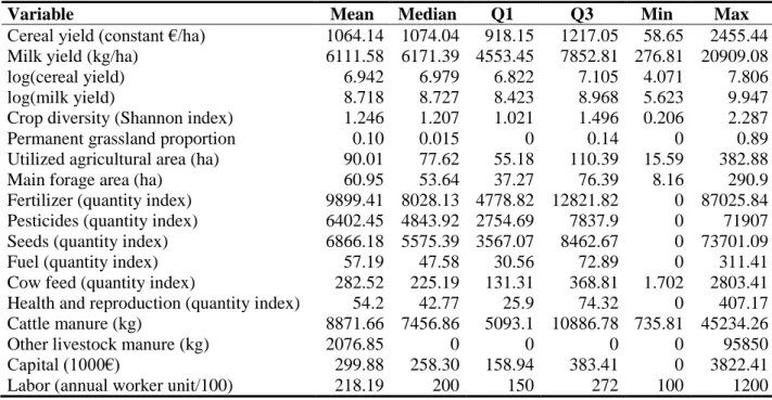
Table 1 presents the descriptive statistics for the farms in the sample. Since the FADN 375

excludes small farms, the average sampled farms had a UAA of 90 ha, which is somewhat 376

18 larger than the French mean. The biodiversity indicators had wide ranges. For example, the 377

maximum value of the crop diversity index was 11 times as large as the minimum value (0.206, 378

which indicates a trend to monoculture). Permanent grasslands were also distributed extremely 379

unequally: 30% of the observations had no permanent grasslands (𝐵𝑖2𝑡= 0). Consequently, we

380

performed a sensitivity analysis in Section 4.3 in which 𝐵𝑖2𝑡 equaled the proportion of

381

permanent grasslands in the UAA of (i) the municipality (LAU2 region),12 _{(ii) district (LAU1}

382

region) or (iii) province (NUTS3 region) of each farm i. Finally, milk and cereals were the most 383

profitable products, providing a mean of 57% and 10% of total revenue, respectively. Some 384

farms had other activities, especially pig production (11% of farms). 385

Table 1. Descriptive statistics of farms (N=3,960)

386

Variable Mean Median Q1 Q3 Min Max

Cereal yield (constant €/ha) 1064.14 1074.04 918.15 1217.05 58.65 2455.44

Milk yield (kg/ha) 6111.58 6171.39 4553.45 7852.81 276.81 20909.08

log(cereal yield) 6.942 6.979 6.822 7.105 4.071 7.806

log(milk yield) 8.718 8.727 8.423 8.968 5.623 9.947

Crop diversity (Shannon index) 1.246 1.207 1.021 1.496 0.206 2.287

Permanent grassland proportion 0.10 0.015 0 0.14 0 0.89

Utilized agricultural area (ha) 90.01 77.62 55.18 110.39 15.59 382.88

Main forage area (ha) 60.95 53.64 37.27 76.39 8.16 290.9

Fertilizer (quantity index) 9899.41 8028.13 4778.82 12821.82 0 87025.84

Pesticides (quantity index) 6402.45 4843.92 2754.69 7837.9 0 71907

Seeds (quantity index) 6866.18 5575.39 3567.07 8462.67 0 73701.09

Fuel (quantity index) 57.19 47.58 30.56 72.89 0 311.41

Cow feed (quantity index) 282.52 225.19 131.31 368.81 1.702 2803.41

Health and reproduction (quantity index) 54.2 42.77 25.9 74.32 0 407.17

Cattle manure (kg) 8871.66 7456.86 5093.1 10886.78 735.81 45234.26

Other livestock manure (kg) 2076.85 0 0 0 0 95850

Capital (1000€) 299.88 258.30 158.94 383.41 0 3822.41

Labor (annual worker unit/100) 218.19 200 150 272 100 1200

4. Results

387

4.1. Log-linear specifications

388

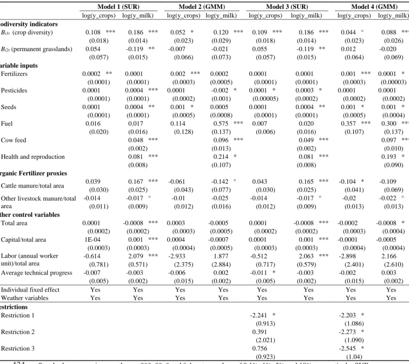
Table 2 presents the estimation of system (2) using Models 1-4. We find that crop diversity 389

(𝐵_𝑖1𝑡) increased both cereal and milk yields in the four models. Permanent grasslands (𝐵_𝑖2𝑡) 390

12 _{LAUs (Local Administrative Units) are building blocks of the NUTS (Nomenclature of Territorial Units for}

19 had no significant effect on cereal yields, which indicates that it had little or heterogeneous 391

productive spillover effects on arable land. The productivity of 𝐵_𝑖1𝑡 estimated by Models 1 and 392

3 (SUR estimates) was twice that estimated by Models 2 and 4 (GMM estimates), which 393

suggested endogenous bias in Models 1 and 3 but also partly supported our assumption that 394

farmers adjust variable input applications given the biodiversity levels. At least, it showed that 395

the instrumentation of the variable inputs disentangled some correlations between them and 396

𝐵𝑖1𝑡. However, Models 1 and 3 highlighted that 𝐵𝑖2𝑡 decreased milk yields.13 Interestingly, the

397

effect became null with Models 2 and 4 once we instrumented the variable input allocations. 398

The lower estimated productivities of 𝐵_𝑖1𝑡 and 𝐵_𝑖2𝑡 in these models highlighted that variable 399

inputs and biodiversity levels were correlated. 400

While productivities of the biodiversity components were our parameters of interest, the 401

literature provided little information about their signs or amplitudes (at least for 𝐵_𝑖2𝑡). In 402

contrast, much more is known about productivities of variable inputs, which are theoretically 403

non-negative (e.g. Carpentier and Letort, 2012). We used this information to discriminate 404

among the four models. Model 1 estimated that all productivities of variable inputs were 405

positive or null, but as mentioned, the estimated productivities of the biodiversity components 406

were likely overestimated due to endogenous biases in variable inputs. Correcting for this issue, 407

Model 2 provides sensibly higher estimates for the productivities of variable inputs (and, thus, 408

lower biodiversity productive capacities).14 The single questionable issue was that the 409

13 _{This result was not surprising: milk-producing farms with a larger proportion of permanent grasslands are}

usually considered the most extensive (Ryschawy et al., 2012).

14 _{Equations of the variable input applications instrumented with prices and subsidies showed R² = 0.16-0.34}

(results available upon request). Price ratios had significant effects and expected signs. In addition, we tested the assumption of short-term optimization by estimating the influence of the other exogenous variables on crop diversity. Ordinary-least-square estimation showed R² = 0.03 in the within form (results available upon request), which suggested little endogenous bias in crop diversity and tended to support the assumption of very short-term optimization.

20 productivity of pesticides for milk was negative,15 perhaps because variable inputs should have 410

been specified as allocable inputs instead of non-allocable inputs.Indeed, for Model 4, the three 411

restrictions added to the productivities of variable inputs differed significantly from zero at the 412

5% level (i.e. they do act as binding constraints). Consequently, all productivities of variable 413

inputs estimated by Model 4 were positive or null, which was consistent with theory. Most 414

importantly, the different specifications for variable inputs did not influence estimates of 415

biodiversity productive capacities (compare Models 2 and 4). Model 3 had similar 416

characteristics but did not correct the endogeneity. Because Model 4 suggests productivities 417

consistent with theory and accounts for endogeneity, we select it as the preferred model. 418

Finally, all fixed inputs had null productivity except UAA, which decreased milk yields: the 419

total area captured the lower per-ha milk yields of extensive farms. The null productivity of 420

other fixed inputs highlighted the difficulty in measuring them accurately. Increasing quantities 421

of cattle manure decreased crop yields, but manure from other livestock had non-significant 422

effects (at the 5% level). This result suggests inefficient management of cattle manure, perhaps 423

because of legislative restrictions on application of organic fertilizers. Specifying alternative 424

organic fertilizer proxies did not influence the significance or the sign of the productivity of 425

𝐵_𝑖1𝑡 or the variable input productivities. Finally, all climatic variables influenced cereal yields 426

significantly (data not shown). In contrast, only total snowfall and minimum, maximum and 427

mean temperatures influenced milk yields. Omitting weather data led to negative productivities 428

of certain variable inputs, highlighting that applications of variable inputs are influenced by the 429

weather. The estimations of Models 1-4 without the individual fixed effects also led to negative 430

15 _{Addition of an interaction variable between pesticide application and a trend highlighted that pesticide}

productivities were positive at the beginning of the period but negative at the end (Appendix 4). This result may have been due to a change in pesticide quality: farmers applied different types of pesticides during the period, and the pesticides that remained by the end may have been less effective. Since milk yields increased over the period, this may have been a temporal conjuncture confound.

21 productivities. The addition of weather variables and individual fixed effects thus decreased the 431

unobserved heterogeneity, removing some endogenous biases. 432

Table 2. Estimates of system (2) with log-linear production functions (Models 1-4) (N=3,960).

433

Model 1 (SUR) Model 2 (GMM) Model 3 (SUR) Model 4 (GMM)

log(y_crops) log(y_milk) log(y_crops) log(y_milk) log(y_crops) log(y_milk) log(y_crops) log(y_milk)

Biodiversity indicators

Bi1t (crop diversity) 0.108 *** 0.186 *** 0.052 * 0.120 *** 0.109 *** 0.186 *** 0.044 ° 0.088 ***

(0.018) (0.014) (0.023) (0.029) (0.018) (0.014) (0.023) (0.026)

Bi2t (permanent grasslands) 0.054 -0.119 ** -0.007 -0.021 0.055 -0.119 ** 0.012 -0.020

(0.057) (0.015) (0.066) (0.073) (0.057) (0.015) (0.064) (0.069) Variable inputs Fertilizers 0.0002 ** 0.0001 0.002 *** 0.0002 0.0001 0.0001 0.001 *** 0.0001 * (0.0001) (0.0001) (0.0003) (0.0005) (0.0001) (0.0001) (0.0003) (0.00003) Pesticides 0.0001 0.0004 *** 0.0001 -0.002 * 0.0001 * 0.0003 * 0.0001 0.0001 (0.0001) (0.0001) (0.0002) (0.001) (0.00005) (0.0002) (0.0002) (0.0002) Seeds 0.0001 0.0004 ** 0.001 * 0.0005 0.0001 0.0004 ** 0.001 * 0.001 * (0.0001) (0.0001) (0.0005) (0.0008) (0.0001) (0.0001) (0.0005) (0.0004) Fuel 0.016 0.017 0.114 0.575 *** 0.007 0.020 0.357 *** 0.300 *** (0.020) (0.016) (0.128) (0.137) (0.006) (0.016) (0.107) (0.137) Cow feed 0.048 *** 0.096 *** 0.049 *** 0.097 *** (0.002) (0.013) (0.002) (0.010)

Health and reproduction 0.081 *** 0.214 * 0.081 *** 0.193 *

(0.008) (0.107) (0.008) (0.090)

Organic Fertilizer proxies

Cattle manure/total area 0.039 0.167 *** -0.061 -0.142 ° 0.043 0.165 *** -0.104 * -0.109

(0.030) (0.025) (0.043) (0.077) (0.030) (0.025) (0.041) (0.069)

Other livestock manure/total area

-0.014 -0.017 ° -0.01 -0.025 -0.014 -0.017 ° -0,02 -0.022 °

(0.011) (0.009) (0.012) (0.016) (0.012) (0.009) (0.013) (0.013)

Other control variables

Total area 0.0001 -0.0008 *** 0.0003 -0.0005 0.0001 -0.0008 *** -0.0002 -0.0008 *

(0.0002) (0.0002) (0.0003) (0.0005) (0.0002) (0.0002) (0.0003) (0.0004)

Capital/total area 1E-04 0.001 *** 0.0004 -0.0007 0.0001 0.001 *** -0.0001 -0.0005

(0.0003) (0.0003) (0.0004) (0.0005) (0.0003) (0.0003) (0.0004) (0.0004)

Labor (annual worker unit)/total area

-0.614 2.079 *** -2.933 1.877 -0.512 2.063 *** -2.898 2.166

(0.781) (0.571) (2.375) (2.884) (0.717) (0.579) (2.401) (2.610)

Average technical progress -0.007 -0.003 -0.006 0.002 -0.011 * -0.003 -0.002 0.003

(0.005) (0.002) (0.015) (0.002) (0.005) (0.002) (0.015) (0.002)

Individual fixed effect Yes Yes Yes Yes Yes Yes Yes Yes

Weather variables Yes Yes Yes Yes Yes Yes Yes Yes

Restrictions Restriction 1 -2.241 * -2.203 * (0.913) (1.086) Restriction 2 0.391 -2.273 * (2.021) (1.090) Restriction 3 0.756 -2.545 * (0.923) (1.04)

Standard errors are in parentheses; ***, **, * and ° denote p-values of 0.1%, 1%, 5% and 10%, respectively. SUR

434

= seemingly unrelated regressions, GMM = general method of moments.

435 436 437

22

4.2. Models with alternative functions

438

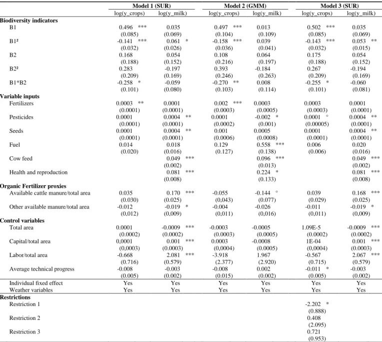
Table 3 presents results of the estimation of Model 4 for system (3) when we added alternative 439

interaction terms for the biodiversity indicators (Appendix 4 presents results of system (3) with 440

Models 1-3). Table 3 includes two degraded forms of system (3) in which either the squared or 441

cross terms of the biodiversity indicators were removed (noted system (3’) and system (3’’), 442

respectively). Second-order parameters of the productivity of 𝐵_𝑖1𝑡 were non-significant for milk 443

once interaction terms were added (system (3)). Adding them even decreased the precision of 444

the estimate of the first-order productivity of milk, except when the squared terms were 445

removed (system (3’’) in Table 3). The results for cereals were more informative. In the most 446

general form, 𝐵_𝑖1𝑡 had a negative return to scale but did have positive productivity at the average 447

point (system (3) in Table 3). The estimates of 𝐵_𝑖2𝑡 and 𝐵_𝑖2𝑡2 were both positive but non-448

significant. The drop in the interaction term between 𝐵_𝑖1𝑡 and 𝐵_𝑖2𝑡 suggested, however, that 449

𝐵𝑖2𝑡 had increasing return to scale (system (3’) in Table 3); in other words, the productivity of

450

𝐵𝑖2𝑡 for cereals was positive when permanent grassland proportions were high (specifically,

451

when 𝐵_𝑖2𝑡 > 0.248, representing ca. 15% of the sample). 452

Finally, the first-order productivity of 𝐵_𝑖2𝑡 was positive for cereals once the squared 453

terms were removed (system (3’’) in Table 3). More interestingly, the two biodiversity 454

indicators interacted negatively with each other for cereal yields, suggesting that they were 455

substitute inputs (systems (3) and (3’’)). 𝐵_𝑖2𝑡 increased cereal yields only when its marginal 456

productivity (0.261-0.217*𝐵_𝑖1𝑡 – system (3’’)) was positive (i.e. when 𝐵_𝑖1𝑡 < 1.20). Based on 457

the distribution of 𝐵𝑖1𝑡, 𝐵𝑖2𝑡 increased cereal yields for 46% of the observations. Similarly, 𝐵𝑖1𝑡

458

increased cereal yields for 89% of the observations (when 𝐵_𝑖2𝑡< 0.35). At the average level of 459

𝐵_𝑖2𝑡, increasing 𝐵_𝑖1𝑡 from an area equally distributed among three crops (𝐵_𝑖1𝑡=1.099) to an area 460

equally distributed among four crops (𝐵_𝑖1𝑡=1.386) increased cereal yields by 2.3% and milk 461

yields by 2.6%. In contrast, 𝐵𝑖2𝑡 did not influence cereal and milk yields at the average level of

23 𝐵_𝑖1𝑡, but it did increase cereal yields at low levels of 𝐵_𝑖1𝑡. When 𝐵_𝑖1𝑡=1, an increase in 𝐵_𝑖2𝑡 463

from 0.1 to 0.2 increased cereal yields by 0.4%, which is relatively small compared to the 464

productivity of 𝐵_𝑖1𝑡. 465

466

Table 3. GMM estimates with log-quadratic production functions (Model 4) (N=3,960)

467

Model 4 – System (3) Model 4 – System (3’) Model 4 – System (3’’)

log(y_crops) log(y_milk) log(y_crops) log(y_milk) log(y_crops) log(y_milk)

Biodiversity indicators Bi1t 0.467 *** -0.043 0.330 *** -0.030 0.077 ** 0.096 ** (0.104) (0.103) (0.094) (0.100) (0.026) (0.028) (Bi1t)² -0.149 *** 0.052 -0.111 ** 0.046 (0.036) (0.038) (0.034) (0.038) Bi2t 0.111 0.051 -0.298 * 0.015 0.261 * 0.042 (0.214) (0.183) (0.138) (0.142) (0.123) (0.13) (Bi2t)² 0.385 -0.075 0.602 ** -0.073 (0.246) (0.224) (0.227) (0.222) Bi1t * Bi2t -0.261 ** -0.040 -0.217 * -0.069 (0.103) (0.108) (0.093) (0.11) Variable inputs Fertilizers 0.001 *** 0.001 ** 0.001 *** 0.001 ** 0.001 *** 0.001 ** (0.0003) (0.0003) (0.0003) (0.0003) (0.0003) (0.0003) Pesticides 0.0001 0.0001 0.0001 0.0001 0.0001 0.0001 (0.0003) (0.0002) (0.0003) (0.0002) (0.0003) (0.0002) Seeds 0.0006 0.0006 0.001 ° 0.001 * 0.001 ° 0.001 * (0.0005) (0.0004) (0.0005) (0.0004) (0.0005) (0.0004) Fuel 0.348 ** 0.293 ** 0.37 ** 0.311 ** 0.34 ** 0.276 ** (0.108) (0.102) (0.108) (0.102) (0.108) (0.09) Cow feed 0.101 *** 0.097 *** 0.099 *** (0.010) (0.010) (0.010)

Health and reproduction 0.205 * 0.207 * 0.193 *

(0.093) (0.091) (0.091)

Organic Fertilizer proxies

Available cattle manure/total area -0.097 * -0.118 ° -0.112 ** -0.102 -0.094 * -0.115 °

(0.041) (0.070) (0.041) (0.070) (0.041) (0.070)

Other available manure/total area -0.013 -0.023 ° -0.018 -0.023 -0.016 -0.022

(0.013) (0.014) (0.013) (0.014) (0.013) (0.013)

Control variables

Total area 0.0002 -0.0009 * 0.0002 -0.0008 ° -2.50E-4 -9.15E-4 *

(0.0002) (0.0004) (0.0002) (0.0004) (2.65E-4) (4.16E-4)

Capital/total area -0.0001 -0.0006 -0.0001 -0.0006 -0.0001 -0.0006

(0.0004) (0.0005) (0.0004) (0.0005) (0.0004) (0.0005)

Labor (annual worker unit)/total area

-3.720 2.372 -2.907 2.149 -3.57 2.45

(2.406) (2.676) (2.420) (2.658) (2.42) (2.63)

Average technical progress -0.006 0.003 -0.007 0.003 -0.002 0.002

(0.015) (0.002) (0.015) (0.002) (0.015) (0.002)

Individual fixed effect Yes Yes Yes Yes Yes Yes

Weather variables Yes Yes Yes Yes Yes Yes

Restrictions Restriction 1 -2.227 * -2.249 * -2.109 * (1.109) (1.112) (1.045) Restriction 2 -2.362 * -2.406 * -2.170 * (1.097) (1.117) (1.044) Restriction 3 -2.419 * -2.551 * -2.310 * (1.045) (1.073) (0.959)

Standard errors are in parentheses; ***, **, * and ° denote p-values of 0.1%, 1%, 5% and 10%, respectively.

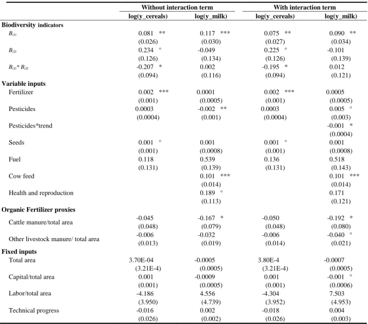
24 When we added interaction terms between variable inputs and biodiversity indicators 469

for cereals, the parameters were less significant for Model 1 (SUR; Appendix 6) and Model 2 470

(Table 4) than for the previous models, but all of the interaction terms were significantly 471

negative (except between fertilizers and 𝐵𝑖2𝑡 in system (5); Table 4).16 This result suggested

472

that the productive capacities of the two biodiversity components were substitute inputs for 473

fertilizers and pesticides. Taking the estimated parameters from system (4), on average, a 10% 474

increase in 𝐵𝑖1𝑡decreased fertilizer and pesticide productivities for cereals by 3.6% and 3.3%

475

respectively. Similarly, a 10% increase in 𝐵_𝑖2𝑡decreased fertilizer and pesticide productivities 476

by 0.6% and 0.9%, respectively. The first-order productivities of the biodiversity indicators 477

remained significant. At average points, productivities of 𝐵_𝑖1𝑡 and 𝐵_𝑖2𝑡 in systems (4) and (5) 478

were consistent with those of systems (2) and (3), confirming that different specifications of 479

variable input allocation did not influence the results. Like for system (2), the productivity of 480

pesticide for milk was negative for systems (4) and (5), but as explained, we could not use the 481

parameter restrictions; the only correction possible was to add an interaction term with a trend, 482

as for system (2) (Appendix 4). 483

484

16 _{Recall that systems (4) and (5) can be estimated only using Models 1 and 2 due to the interaction terms between}

25

Table 4. GMM estimates of systems (4) and (5) (Model 2) (N=3,960)

485

Model 2 – System (5) Model 2 – System (4)

log(y_crops) log(y_milk) log(y_crops) log(y_milk)

Biodiversity indicators Bi1t -0.056 0.105 0.929 *** 0.113 *** (0.039) (0.102) (0.248) (0.025) (Bi1t)² 0.577 ** 0.002 2.804 *** 0.063 (0.203) (0.037) (0.589) (0.054) Bi2t 2.090 * 0.164 (0.839) (0.184) (Bi2t)² -0.964 -0.254 (0.758) (0.210) Bi1t * Bi2t -0.314 0.025 (0.235) (0.106) Variable inputs Fertilizers 0.007 ** 0.0001 0.007 ** 0.0001 (0.002) (0.0004) (0.002) (0.0004) Fertilizers*Bi1t -0.004 * -0.004 * (0.002) (0.002) Fertilizers*Bi2t -0.002 -0.011 *** (0.003) (0.003) Pesticides 0.023 *** -0.002 * 0.013 ** -0.002 * (0.004) (0.001) (0.004) (0.001) Pesticides*Bi1t -0.013 ** -0.006 * (0.003) (0.003) Pesticides*Bi2t -0.022 * -0.030 *** (0.007) (0.008) Seeds 0.001 0.002 ** 0.001 0.002 ** (0.001) (0.0007) (0.001) (0.0007) Fuel 0.009 0.443 *** 0.190 0.441 *** (0.156) (0.128) (0.157) (0.128) Cow feed 0.069 *** 0.068 *** (0.013) (0.012)

Health and reproduction 0.261 ** 0.236 **

(0.087) (0.084)

Organic Fertilizer proxies

Available cattle manure/total area -0.081 -0.066 0.037 -0.053

(0.055) (0.071) (0.058) (0.069)

Other available manure/total area 0.008 -0.018 0.019 -0.018

(0.006) (0.016) (0.019) (0.016) Control variables Total area 0.0003 -0.0004 -0.0003 -0.0006 (0.0005) (0.0005) (0.0005) (0.0005) Capital/total area -0.0008 -0.0002 -0.0003 -0.0004 (0.0006) (0.0005) (0.0005) (0.0005) Labor/total area -0.607 0.469 -8.440 1.863 (6.067) (4.895) (6.079) (4.892)

Average technical progress 0.001 0.002 0.001 0.002

(0.002) (0.002) (0.002) (0.002)

Individual fixed effect Yes Yes Yes Yes

Weather variables Yes Yes Yes Yes

Standard errors are in parentheses; ***, **, * and ° denote p-values of 0.1%, 1%, 5% and 10%, respectively.

486 487

4.3. Sensitivity analysis for permanent grasslands

488

The choice of indicators depends greatly on the data available. Using the FADN database 489

required us to rely on indicators calculated at the farm scale; however, landscape ecologists 490

suggest that the scale at which these indicators are calculated matters (Burel and Baudry, 2003). 491

26 Although Donfouet et al. (2017) emphasized that the scale at which 𝐵_𝑖1𝑡 was calculated had no 492

significant influence on the assessment of the productivity of 𝐵𝑖1𝑡 in previous studies, we were

493

not aware of such evidence 𝐵_𝑖2𝑡. We thus tested whether the scale at which the permanent 494

grassland proportion was measured had an influence by estimating system (2) with alternative 495

measures of 𝐵_𝑖2𝑡. Formally, we replaced 𝐵_𝑖2𝑡 with the proportion of permanent grasslands in 496

the UAA of the (i) municipality, (ii) district or (iii) province where the farmstead of i was 497

located. This sensitivity analysis had the secondary advantage that 𝐵_𝑖2𝑡 was always positive at 498

these scales, which was not the case at the farm scale (Table 1). The disadvantage was that we 499

had to decrease the number of observations from 3,960 to 2,344 since these alternative measures 500

of 𝐵_𝑖2𝑡 have been available only since 2007 in France (beginning of the Land Parcel 501

Identification System). 502

Using Model 4 to estimate system (2) with 𝐵𝑖2𝑡 measured at alternative scales revealed

503

that biodiversity productive capacity remained similar overall to that estimated at the farm scale 504

(Table 5). Although the amplitudes differed, 𝐵_𝑖1𝑡 still increased cereal and milk yields. The 505

alternative measures of 𝐵_𝑖2𝑡 did not influence estimates of the productivity of 𝐵_𝑖1𝑡. The lack of 506

effect of 𝐵𝑖2𝑡 on cereal yields also remained, but the alternative measures of 𝐵𝑖2𝑡 influenced all

507

milk yields negatively (and significantly). The proportion of permanent grasslands at the district 508

level influenced the results the most. Estimating system (2) using all alternative measures of 509

permanent grasslands at the same time, the alternative measures of permanent grasslands again 510

had no effect on the productivity of 𝐵_𝑖1𝑡 for cereals and milk (Appendix 7). We confirmed that 511

the proportion of permanent grasslands at the district level drove the negative effect on farms’ 512

milk yields. Estimates of variable input productivities had lower quality (Table 5), however, 513

than those of previous models due to the smaller sample size. 514