HAL Id: halshs-00639731
https://halshs.archives-ouvertes.fr/halshs-00639731
Submitted on 9 Nov 2011
HAL is a multi-disciplinary open access
archive for the deposit and dissemination of sci-entific research documents, whether they are pub-lished or not. The documents may come from teaching and research institutions in France or
L’archive ouverte pluridisciplinaire HAL, est destinée au dépôt et à la diffusion de documents scientifiques de niveau recherche, publiés ou non, émanant des établissements d’enseignement et de recherche français ou étrangers, des laboratoires
Existence, Optimality and Dynamics of Equilibria with
Endogenous Time Preference
Cuong Le Van, Cagri Saglam, Selman Erol
To cite this version:
Cuong Le Van, Cagri Saglam, Selman Erol. Existence, Optimality and Dynamics of Equilibria with Endogenous Time Preference. Journal of Mathematical Economics, Elsevier, 2011, 47 (2), pp.170-179. �halshs-00639731�
Existence, Optimality and Dynamics of Equilibria
with Endogenous Time Preference
Cuong Le Van
∗Cagri Saglam
†Selman Erol
‡July 2009
Abstract
To account for the development patterns that differ considerably among economies in the long run, a variety of one-sector models that incorporate some degree of market imperfections based on technolog-ical external effects and increasing returns have been presented. This paper studies the dynamic implications of, yet another mechanism, the endogenous rate of time preference depending on the stock of capital, in a one-sector growth model. The planner’s problem is presented and the optimal paths are characterized. We show that development or poverty traps can arise even under a strictly convex technology. We also show that even under a convex-concave technology, the optimal path can exhibit global convergence to a unique stationary point. The multipliers system associated with an optimal path is proven to be the supporting price system of a competitive equilibrium under external-ity and detailed results concerning the properties of optimal (equilib-rium) paths are provided. We show that the model exhibits globally monotone capital sequences yielding a richer set of potential dynamics than the classic model with exogenous discounting.
Keywords: Endogenous time preference; Optimal growth; Competi-tive equilibrium; Multiple steady-states
JEL Classification Numbers: C 61; D90; O41
∗PSE, CNRS, University Paris 1, CES, France. e-mail: [email protected]
†Department of Economics, Bilkent University, Turkey. e-mail: [email protected] ‡Department of Economics, Bilkent University, Turkey. e-mail: [email protected]
1
Introduction
The optimal capital accumulation models have been at the core of the theory of economic growth and dynamics. Based on the dynamic consumption and saving decisions of the economic agents driven by intertemporal utility trade-offs between current and future consumption, the key components of these models turn out to be the rate of time preference and the technology. The classical optimal growth models and much of the subsequent literature on growth focus on the convex structures of the technology and preferences that guarantee the monotonical convergence of the sequence of optimal stocks towards a unique steady state. Such a structure however imply that the model cannot be used to understand the development patterns that differ considerably among countries in the long run (see Quah, 1996; Barro, 1997; Barro and Sala-i-Martin, 1991).
To account for these non-convergent growth paths, a variety of one-sector optimal growth models that incorporate some degree of market im-perfections based on technological external effects and increasing returns have been presented. Within a model of capital accumulation with convex-concave technology, Dechert and Nishimura (1983), Mitra and Ray (1984) have characterized optimal paths and prove the existence of threshold effect that generates development or poverty traps (see Azariadis and Stachurski, 2005, for a recent survey). In these models, economies with low initial capi-tal stocks or incomes converge to a steady state with low per capita income, while economies with high initial capital stocks converge to a steady state with high per capita income. Indeed, the introduction of increasing returns also makes it possible for private returns to the accumulation of capital stock to be complementary with the aggregate stock leading to indeterminacies or continuum of equilibria (e.g., Benhabib and Perli, 1994; Benhabib and Farmer, 1996; see Nishimura and Venditti, 2006 for extensive bibliography). A general tendency in these studies with multiple steady states, inde-terminacy or continuum of equilibria is that they are mostly devoted to the analysis of the technology component leaving the time preference essentially unaltered with an exogenously fixed geometric discounting. In this paper, yet the other mechanism, the endogeneity of time preference will be put for-ward to explain theoretically why the differences in per capita output levels among countries persist in the long run.
Considering the preferences of the agents to be recursive, the early con-tributions on the theory of endogenous time preference postulate that an
agent’s discount rate depends on the level of present and future consump-tion (e.g., Uzawa, 1968; Lucas and Stokey, 1984; Epstein, 1987; Obstfeld, 1990). These models nearly exclusively assume an increasing marginal im-patience so that the agents get more impatient as they grow richer. Such a specification ensures stable optimal capital sequences that converge to a unique steady state independent of the initial conditions. However, recent work both theoretically (e.g., Becker and Mulligan, 1997; Stern, 2006) and empirically (e.g., Lawrence, 1991; Samwick, 1998; Frederick et al., 2002) propose that the agents get more patient as they grow richer and impose that the discount rate depends closely upon the stock of wealth (see Hamada and Takeda, 2009, for a recent survey). By considering discount factor as a function of consumption, Mantel (1998) studies the impact of decreas-ing rate of time preference on optimal growth path of an economy with a primary focus on the monotonicity properties of optimal consumption and investment. Stern (2006), along the lines of Becker and Mulligan (1997), let individuals spend resources to increase the appreciation of the future. He provides numerical examples of multiple steady states and a conditionally sustained growth path.
In this paper we adapt the classic optimal growth model to include an endogenous rate of time preference depending on the stock of capital and analyze the implications on the equilibrium dynamics. To do so, the plan-ner’s problem is first presented and the optimal paths are characterized. We show that development or poverty trap can arise even under a strictly con-vex technology. In other words, we prove that there exists a critical value of initial stock, in the vicinity of which, small differences lead to perma-nent differences in the optimal path. On the other hand, we also show that even under a convex-concave technology, the optimal path can exhibit global convergence to a unique stationary point. Later, the multipliers system as-sociated with an optimal path is proven to be the supporting price system of a competitive equilibrium under externality and detailed results concerning the properties of optimal (equilibrium) paths are provided. We show that the model exhibits globally monotone capital sequences yielding a richer set of potential dynamics than the classic model with exogenous discounting.
The key feature of our analysis is to consider that the rate of time pref-erence decreases with the stock of wealth in contrast with exogenously fixed discount factor assumed in standard models. Accordingly, the lower the stock of capital , the higher the sacrifice of postponing present consumption in exchange for future consumption. An important aspect of our model is
that while allowing variation in the rate of time preference, at the same time it maintains time consistency. A remarkable feature of our analysis is that it does not rely on particular parameterization of the exogenous functions involved in the model, rather, it provides a more flexible framework in re-gards to the discounting of time, keeps the model analytically tractable and uses only general and plausible qualitative properties.
The rest of the paper is organized as follows. Section 2 describes the model and provides the dynamic properties of optimal paths. Section 3 presents the existence of a competitive equilibrium with externality and studies the equilibrium dynamics. Some more technical proofs are given in Appendix.
2
Model
The model differs from the classic optimal growth model by the assump-tions on discounting. Rather than assuming that the level of discount on future utility is an exogenous parameter, we assume that it is endogenous depending on the path of capital stock. Formally, the model is stated as follows: max {+1}∞=0 ∞ X =0 Ã Y =1 () ! () (P) subject to ∀ + +1≤ () ∀ ≥ 0 ≥ 0 0≥ 0 given,
We make the following assumptions regarding the properties of the discount, utility and the production functions.
Assumption 1 : R+ → R++ is continuous, differentiable, strictly
in-creasing and satisfies sup0 () = 1 sup00() +∞
Assumption 2 : R+ → R+ is continuous, twice continuously
differen-tiable and satisfies (0) = 0 Moreover, 0 0 (strictly increasing), 00 0 (strictly concave) and 0(0) = +∞ (Inada condition).
Assumption 3 : R+ → R+ is continuous, twice continuously
For any initial condition 0 ≥ 0 when x = (0 1 2 ) is such that
0 ≤ +1 ≤ () for all we say it is feasible from 0 and the class
of all feasible accumulation paths is denoted by Π (0) It may be easily
verified that if 0
0
0 then Π (0) ⊂ Π
³
00´ A consumption sequence c = (0 1 ) is feasible from 0 ≥ 0 when there exists x ∈ Π (0) with
0 ≤ ≤ () − +1 and the class of consumption sequences feasible from
0 is denoted byP(0)
Noting that the constraints will be binding at the optimum as utility and the discount function is strictly increasing, we introduce the function defined on the set of feasible sequences as
(x) = ∞ X =0 Ã Y =1 () ! ( () − +1) (1)
The preliminary results are summarized in the following Lemma which has a standard proof (see Le Van and Dana, 2003; Duran and Le Van, 2002 and Stokey and Lucas, 1989).
Lemma 1 If 0(0) ≤ 1 let − = 0 If 0(0) 1 let − be the largest point 0 such that () = . Then,
(a) For any x ∈ Π (0) we have ≤ (0) for all where (0) =
maxn0−
o
(b) Π (0) is compact in the product topology defined on the space of
sequences x
(c) is well defined and it is continuous over Π (0) with respect to the
product topology.
It can be easily observed that (a) follows from the existence of a maxi-mum level of sustainable capital stock. Such a point,− exists since 0(∞) 1 With this bound and Tychonov theorem, (0)∞ is a compact
topolog-ical space. Π (0) is closed subset of (0)∞, hence compact. is well
defined since (0) puts also a bound on the feasible consumption and
sup0 () = 1 The continuity of follows from the continuity of
the functions together with the bound on discounting, 1
It is now clear that the initial optimal growth model is equivalent to:
max{ (x) : x ∈ Π (0)} (P0)
2.1
Existence of Optimal Paths
The existence of an optimal path follows from the fact that Π (0) is compact
con-tinuous for this product topology. The positiveness of optimal consumptions and capital stocks follows from the Inada condition.
Proposition 1 (i) There exists an optimal path x The associated optimal consumption path, c is given by
= () − +1 ∀
(ii) If 0 0, every solution (x c) to the optimal growth model satisfies
0 0 ∀ (2)
Proof: See Appendix.
2.2
Value Function, Bellman Equation, Optimal Policy
In order to characterize the behavior of the optimal paths, we will proceed by defining the value function and analyzing the properties of the optimal policy correspondence. The value function is defined by:
∀0 ≥ 0 (0) = max {+1}∞=0 ( ∞ X =0 Ã Y =1 () ! ( () − +1) ¯ ¯ ¯ ¯ ¯ ∀ 0 ≤ +1≤ () 0 ≥ 0 } (3)
The bounds on discounting together with the existence of maximum sustainable capital stock guarantee a finite value function. Under the As-sumptions (1) and (2), one can immediately show that the value function is non-negative, strictly increasing and continuous. Given these, the satisfac-tion of Bellman’s equasatisfac-tion easily follows.
Proposition 2 (i) (0) = 0, and (0) 0 if 0 0. If x is the optimal
path, then (0) = ∞ X =0 Ã Y =1 () ! ( () − +1)
(ii) is strictly increasing. (iii) is continuous.
Proposition 3 (i) satisfies the following Bellman equation: ∀0 ≥ 0 (0) = max
{((0) − ) + () () | 0 ≤ ≤ (0)} (4)
(ii) A sequence x ∈ Π (0) is an optimal solution if, and only if, it
satisfies:
∀ () = ( () − +1) + (+1) (+1) (5)
Proof: See Appendix.
The optimal policy correspondence, : R+→ R+ is defined as follows:
(0) = arg max {((0) − ) + () () | ∈ [0 (0)]}
It is important to note that although the utility function is strictly concave, the solution may not be unique as the multiplication of discount function destroys the concave structure needed for uniqueness. The non-emptiness and the closedness of the optimal correspondence and its equiv-alence with the optimal path follow easily from the continuity of the value function by a standard application of the theorem of the maximum.
Proposition 4 (i) (0) = {0}
(ii) If 0 0 and 1 ∈ (0) then 0 1 (0)
(iii) is upper semi-continuous.
(iv) A sequence x ∈Π (0) is optimal if and only if +1∈ () ∀
(v) The optimal correspondence is increasing so that if 0 00 1 ∈
(0) and 01∈ (00) then 1 01
Proof: See Appendix.
The increasingness of is crucial for the convergence of optimal paths, hence for the analysis of the long-run dynamics. In Stern (2006), assuming an endogenous time preference depending on the future-oriented resources, the increasingness of has been proven by using the strict concavity of Such a restriction on the curvature of the discount function is not necessary in our setup. Moreover, we have also proven that the optimal correspon-dence, is not only closed but also upper semi-continuous.
With the positiveness of the optimal consumptions and capital stocks, the fact that the optimal capital stocks satisfy the Euler equation easily follows.
Proposition 5 When 0 0 any solution x ∈ Π (0) satisfies the Euler
equation:
∀ 0( () − +1) =
(+1) 0( (+1) − +2)0(+1) + 0(+1) (+1) (6)
Proof: See Appendix.
In a standard optimal growth model with geometric discounting and the usual concavity assumptions on preferences and technology, the optimal policy correspondence, is single valued and the properties of the optimal path is easily found by using the first order conditions together with enve-lope theorem by differentiating the value function. However, in our model, the objective function includes multiplication of a discount function. This generally destroys the usual concavity argument which is used in the proof of the differentiability of value function and the uniqueness of the optimal paths (see Benveniste and Scheinkman, 1979; Araujo, 1991). Indeed, incor-porating an endogenous time preference depending on the future-oriented resources, even with strict concavity assumed for the discount function, the differentiability, hence the uniqueness of the optimal paths are left as open questions in Stern (2006).
To this end, we shall prove that the value function is differentiable almost everywhere and there exists a unique optimal path from almost everywhere without any assumption on the curvature of . In doing so, one may easily refer to the Clarke generalized gradients (see Askri and Le Van, 1998). How-ever, for the sake of comparability with the tools used in standard optimal growth models, we proceed with proofs analogous to those in Le Van and Dana (2003).
Proposition 6 (i) Left derivative of exists at every 0 0 and −0(0) =
0( (0) − (0))0(0) where (0) = min (0)
(ii)Right derivative of exists at every 0 0 and +0(0) = 0( (0) −
Θ(0))0(0) where Θ(0) = max (0)
Proof: See Appendix.
Now we are able to see the relation between differentiability of the value function and the uniqueness of the optimal path. Notice that, given 0 if
from the above proposition, we see that −0(0) = +0(0) hence is
dif-ferentiable at 0 and vice-versa. This analysis obviously can be generalized
to any period other than 0 These allow us to claim that the optimal correspondence is single valued and differentiable almost everywhere. Proposition 7 (i) If x is an optimal path from 0 then is differentiable
at any ≥ 1 If x is an optimal path from 0 there exists a unique
optimal path from for any ≥ 1
(ii) is differentiable at 0 0 if and only if there exists a unique
optimal path from 0
(iii) is differentiable almost everywhere, i.e., the optimal path is unique for almost every 0 0
(iv) is differentiable almost everywhere. Proof: See Appendix.
We have proved that the optimal correspondence is single valued and differentiable almost everywhere. In addition to this, we have also shown that there exists a unique optimal path from almost any initial capital stock. These results will prove to be crucial in analyzing the dynamic properties of the optimal paths.
2.3
Dynamic Properties of the Optimal Paths
A point is an optimal steady state if = () so that the stationary sequence x = ( ) solves the problem: max{ (x) : x ∈ Π ()} If is different from zero, then the associated optimal steady state consumption must be strictly positive from Inada condition. Hence, from Euler equation (6), this steady state will solve:
0( () − ) = () 0( () − )0() + 0() () (7) By Proposition 3, we know that the stationary plan every period equal to is optimal from if and only if it satisfies
() = ( () − ) + () () (8) Following from (7) and Euler equation (8), this steady state will satisfy:
( () − ) = [1 − ()][1 − ()
0()]
We will now prove that the endogenous rate of time preference preserves the monotonicity of the optimal paths and provide the condition under which the convergence to an optimal steady state is guaranteed.
Proposition 8 The optimal capital stocks path x from 0 is monotonic.
Proof: Since is increasing, if 0 1 we have 1 2 By induction,
+1 ∀ If 1 0 using the same argument yields +1 ∀
Now if 1 = 0 then 0 ∈ (0) Recall that the optimal path is unique
after = 1 Since 0 ∈ (0) = 0 ∀
It is important to note that the monotonicity of the optimal paths has been proved without any assumption on the curvature of neither the produc-tion nor the discount funcproduc-tion. It is already well known that in multi-sector nonclassical optimal growth models, one can easily refer to lattice program-ming and Topkis theorem in order to prove that the optimal paths are monotonic if the planner’s criterion function is supermodular (see Amir, et al., 1991). However, following this approach in a model with time preference depending on the future-oriented resources, Stern (2006) assumes a strictly concave discount function.
As a monotone real valued sequence will either diverge to infinity or converge to some real number, the fact that optimal capital sequences are monotone proves to be crucial in analyzing the dynamic properties and the long-run behavior of our model.
Proposition 9 If sup00() 1−_
for some small enough, then any
optimal path converges to zero.
Proof: Let the optimal path x converge to 0. Then, by considering the Euler equation as → ∞, we obtain
( () − ) 0( () − ) = [1 − ()][1 − ()0()] 0() ≥ 1 − _ 0 sup [1 − _ sup00()]
where sup0 ≡ sup00() Note that (0)0 =
(0)2−00
(0)2 0 i.e.
0 is
increasing. Let = arg max0( () − ) Accordingly, it is clear that
( () − ) 0( () − ) ≥ ( () − ) 0( () − ) ≥ 1 − _ 0 sup [1 − _ sup00()]
Defining = sup0 1− _ ( ()−) 0( ()−) sup00() ≥ 1−_
when the optimal path
converges to 0 Thus, sup00() 1−_
implies that the optimal path
converges to zero.
In a classic optimal growth model, if 0(0) ≤ 1
then the optimal path
converges to zero. As we consider the endogenous nature of time preference and allow for nonconvexities in the production technology, we have slightly deviated from this condition. However, it must be noted that the interval for sup00() that guarantees the convergence to zero will always be a subset of
µ 0−1
¶
and this can not be improved in an essential way.
We will now present the condition under which the convergence to an optimal steady state is guaranteed and analyze the behavior of the optimal paths when we would have unique or multiple optimal steady states. Proposition 10 Assume 0 0 Let inf0 () =
−
If 0(0) 1
−
then the optimal path converges to an optimal steady state 0.
Proof: Since (·) is increasing,
−
= (0) Note that (0) (·) is a continu-ous function and 0(0)(0) 1 Assume that x is an optimal path and it converges to zero. Since 0 is continuous, there exists such that implies 0()() 1
If x is an optimal path then it satisfies the Euler equation. Hence, for every in particular, for we have:
0( () − +1) = 0( (+1) − +2)(+1)0(+1) + 0(+1) (+1) 0( (+1) − +2)(+1)0(+1) 0( (+1) − +2) implying that 0( () − +1) 0( (+1) − +2) and () − +1 (+1) − +2
Then, we obtain that:
0 () − lim
→0 () − = 0
leading to a contradiction.
Since the sequence x is monotonic, it converges to some 0. The upper semi-continuity of the correspondence implies ∈ ()
With convex technology and exogenously fixed time preference rate in a standard optimal growth model, if 0(0) 1 then there exists a unique (non-zero) steady state to which all optimal paths converge independently of their initial state. In our model, thanks to the existence of the maxi-mum sustainable level of capital stock, when 0(0) 1
−
the optimal path converges monotonically towards an optimal steady state. This condition can easily be recast as 0(0) + by defining the rate of interest by
1(1 + ) =
−and the function by () = () + (1 − ) where is the
production function and is the rate of depreciation of capital. Accordingly, in our model, when the cost of investment is low, the optimal capital stocks converge to an optimal steady state.
We will now consider the optimal path dynamics in the long run and show that our model can support unique optimal steady state with global convergence and multiplicity of optimal steady states with local convergence. Indeed, we will show that our model exhibits global convergence even under convex-concave technology and multiplicity of optimal steady states even under convex technology due to the endogenous nature of time preference. Case 1 (Global Convergence)Assume 0 0 Let inf0 () =
−
and 0(0) 1
−
Consider the case where there exists a unique solution to (9). By Proposition 10, we know that the optimal paths can not converge to 0 Then, any optimal path converges to the unique optimal steady state , irrespective of their initial state.
The answer to this question will enable us to show whether an econ-omy with wealth dependent endogenous discounting can exhibit threshold dynamics even under a convex technology as well.
Case 2 (Local Convergence) Assume 0 0 Let inf0 () = −
and 0(0) 1
−
We will now consider the case where we have multiple solu-tions to the steady-state equation (9). The stationary sequences associated with these steady states may or may not be optimal. A natural question is then whether these solutions will constitute the long-run equilibrium in the optimal growth model. Consider the case where we have exactly two optimal steady states, , for the sake of simplicity. Suppose that is unstable.
Given the existence of a maximum sustainable capital stock, as any optimal path from 0 has to converge to an optimal steady state, there will be
another steady state larger than a contradiction. Hence, is locally
stable. It is also impossible to have unstable, since the optimal paths can
not converge to 0 However, note that whenever both of these optimal steady states turn out to be saddle-point stable, that would imply the existence of a critical stock and the emergence of threshold dynamics.
The following proposition provides the formal analysis of the local con-vergence under two optimal steady states.
Proposition 11 Given that the high and the low optimal steady states are respectively and , there exists ∈ ( ) such that any optimal path x
starting from 0 converges to if 0 and converges to if 0
Proof: Take any initial capital levels and let the corresponding optimal paths be y z Since the optimal correspondence is increasing,
hence lim→∞ ≤ lim→∞Thus, if z converges to so does y If
y converges to so does z. Let ∗1 = sup{| the optimal path from
converges to } and ∗2= inf{| the optimal path from converges to }
Clearly from the above argument, ∗1 = ∗2 Then, posing ∗ = ∗1 = ∗2 completes the proof.
Actually, the existence of critical value is recognized since the papers by Clark (1971), Majumdar and Mitra (1982), Dechert and Nishimura (1983) in discrete time and Skiba (1978) and Askenazy and Le Van (1999) in continu-ous time horizon. It is important to note that all of these studies are devoted to the analysis of the technology component leaving the time preference es-sentially unaltered with an exogenously fixed geometric discounting. They assume a specific convex-concave technology under which the low steady state turns out to be unstable and high steady state turns out to be stable so that an optimal path converges either to zero or to the high steady state. However, we show that even under strictly concave production function, the economy can exhibit a "trap" so that a critical value of the initial stock will exist, in the vicinity of which, small differences will lead to permanent differences in the optimal path. An optimal path converges either to the low or the high steady states which turn out to be saddle-point stable. Com-pared to the optimal growth models with exogenous time preference, this introduces a fundamental difference in the optimal path dynamics.
We must make one point very clear. Our results are general in the sense that it does not assume any specific functional forms for the production and the discount functions. Stern (2006), incorporating an endogenous time preference depending on the future-oriented resources, analyzes a series of numerical examples that also exhibit multiplicity of steady states with mere local convergence. In order to provide a better exposition of our analysis, following Stern (2006), we will specify functional forms in an example and show that our model supports multiplicity of optimal steady states with local convergence.
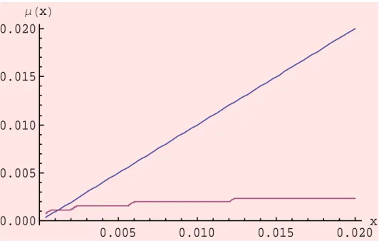
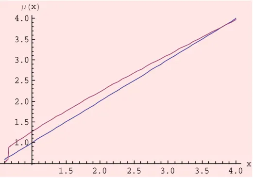
Example 1 Suppose that () = + (1 − ) () = 1−1− and () = −−(+) where 0 { } 0 { } 1 0 and − 1 Check that , , satisfy the assumption sets. We employ the fol-lowing set of coefficients:
= 05 = 03 = 015 = 05 = 097 = 25 = 1 = 09 It turns out that the maximum sustainable capital stock − is 55843, and there exist three solutions to (9). The precise values are, = 00012,
= 05865 and = 38106. In order to determine which of these are
indeed optimal steady states we analyze the optimal policy by making use of Bellman’s operator. Figure 1 shows the optimal policy for iterations of the Bellman operator on the zero function and indicates that and are
saddle point stable optimal steady states. Figure 2, 3 and 4 present the de-tailed picture of the optimal policy in the neighborhood of the and
respectively. In contrast with Stern (2006), even though is a solution of
the stationary Euler equation (9), Figure 1 strongly indicates that it is not an optimal steady state. In the light of our analysis, for any initial capital stock level lower than a critical stock, the system will face a development trap, enforcing convergence to a very low capital level ≈ 00012, even
under a strictly concave production function.
3
Existence of a Competitive Equilibrium with
Ex-ternality
From now on, we will assume that the production function is strictly concave. We first define the concepts of equilibrium with externality and competitive equilibrium. Suppose we are given a sequence of capital ˜x =
(0 ˜1 ˜ ) ∈ [0 (0)]∞ and the associated sequence of discount
fac-tors ˜ = ( ˜1 ˜ ) where ˜ = (˜) ∀ ≥ 1 Given this fixed sequence
˜ ∈ ∙ − ¯ ¸∞
consider the following problem:
max x ∞ X =0 Ã Y =1 ˜ ! ( () − +1) (PE) subject to ∀ 0 ≤ +1≤ () 0 0 given
The solution x = (0 1 ) to this problem depends on ˜, hence ˜x
We write x = ³
˜ ´
= ( (˜x)) and hence x = Φ (˜x) An equilibrium with externality is a sequence of capital stock x∗ = (0 ∗1 ∗ ) such that
x∗= Φ (x∗) A list of sequences (x∗ c∗ p∗ ∗) is a competitive equilibrium
with externality of this economy if the following are satisfied: a) c∗ ∈ ∞+ x∗∈ ∞+ p∗∈¡1+\ {0}¢ ∗ ∈ R++
b) c∗ solves the consumer’s problem:
max c ∞ X =0 Ã Y =1 (∗) ! () (CP) subject to ∞ X =0 ∗≤ ∗0+ ∗
where ∗ is the maximum profit of the firm, c) x∗ solves the firm’s problem:
∗= max x ∞ X =0 ∗( () − +1) − ∗0 (PP) subject to ∀ ≥ 0 0 ≤ +1≤ () 0 0 given
d) and the markets clear at every period:
The purpose is to prove the existence of a competitive equilibrium of this intertemporal economy. To do so, we will first prove that there exists a fixed point of Φ namely an equilibrium. Later, under an additional assumption, we will show that this equilibrium is indeed a competitive equilibrium of the intertemporal economy with endogenous time preference.
The value function associated with the problem (PE) takes the following form: (0 1 2 3 ) = max x ∞ X =0 Ã Y =1 ! ( () − +1) subject to 0 ≤ +1≤ () 0 0 given
clearly satisfies the Bellman equation: ( +1 +2 ) = max
∈[0 ()][( () − ) + +1 ( +2 +3 )]
Proposition 12 The function is continuous with the topology in R for 0
and the product topology for ∈ ∙
−
¯ ¸∞
. Moreover, it is strictly concave.
Proof: Let (0 x) = ∞ X =0 Ã Y =1 ! ( () − +1)
where x ∈ Π(0). It is easy to show that is continuous in (0 x) for
the topology in R for 0 and the product topology for ( x). It is
well-known that Π(·) is a continuous correspondence from R+ into the space of
sequences endowed with the product topology (see e.g. Le Van and Dana, 2003). Since
(0 ) = max {(0 x)|x ∈ Π(0)}
from the maximum theorem, is continuous. The strict concavity of with respect to 0 follows from the strict concavity of and .
Lemma 2 The map is continuous with respect to the product topology. Proof: Standard.
Proposition 13 Φ is continuous with respect to the product topology. Proof: From the maximum theorem, the solution x is upper semi-continuous with respect to . As the solution to (PE) is unique, x is continuous with respect to . Since ˜ = (˜x), the map Φ is continuous with respect to ˜x by Lemma (2).
To attain an equilibrium, the initial sequence of discounting has to be consistent with the level that is assumed when the agent makes her sin-gle decisions. This suggests that the fixed points of Φ are candidates for equilibria.
Proposition 14 Φ has a fixed point.
Proof: Φ is a continuous mapping from [0 (0)]∞into [0 (0)]∞. Since
this one is compact for the product topology and convex, from the Schauder theorem, there exists x∗ ∈ [0 (0)]∞which satisfies x∗ = Φ(x∗).
Proposition 15 Any fixed point x∗ of Φ satisfies the Euler equation:
0( (∗) − ∗+1) = 0( (∗+1) − ∗+2)(∗+1)0(∗+1) (10) Proof: Standard.
For the rest, we assume that the function [0](·) is decreasing and [0](0) 1. Note that lim→∞[0]() 1
Proposition 16 The equilibrium with externality, namely the fixed point of Φassociated with 0 is unique.
Proof: Suppose not. Let (0 01 02 ) and (0 001 002 ) be two fixed
points with 01 001 Let the associated consumption paths be (00 01 ) and (000 001 ).
First, we will prove by induction that 0 00 for all ≥ 1 and 0 00 for all . Trivially, 00 = (0) − 01 (0) − 001 = 000 Then by (10),
0(01)[0](10) = 0(00) 0(000) = 0(001)[0](001) which implies 0(01) 0(00
1) as [0] is a decreasing function. Hence, 01 001.
Now suppose 0 00 and 0 00 for some (0) − 0+1 = 0 00 = (00) − 00+1, so 0+1 00+1 Again, by (10), 0(0+1)[0](0+1) = 0(0)
0(00) = 0(00+1)[0](+100 ) which implies 0(0+1) 0(00+1) as [0] is a decreasing function. Hence, 0
+1 00+1 and 0+1 00+1
Notice that given the discounting sequence (x0) x00is feasible and yields higher utility than x0 which is a contradiction with the optimality of x0given (x0) Therefore, equilibrium is unique.
Proposition 17 The fixed point x∗of Φ monotonically converges to a point satisfying [0]() = 1. Moreover, in case of multiplicity of such points, x∗ monotonically converges to the one closest to 0.
Proof: First, consider the case [0](·) is strictly decreasing. Let be the unique "steady state" capital stock satisfying [0]() = 1
Suppose that for some , ∗ ∗+1 and ≤ ∗+1 are satisfied. Then (10) implies 0(∗
) ≤ 0(∗+1) i.e. (∗) − ∗+1 ≥ (∗+1) − ∗+2 Hence,
∗+1 ∗+2 and +2∗ So inductively we obtain ∗+1 ∗+2 . Due to the maximum sustainable capital stock, x∗ cannot diverge so converges to a level higher than However, x∗ is a fixed point, so the
optimal path given the discounting sequence consistent with the path itself can only converge to by (10), yielding a contradiction.
Similar arguments apply for the case ∗ ∗+1 and ≥ ∗+1 at which we end up with x∗ converging to 0, which is again impossible because then (x∗) would converge to
−
and Inada condition would prevent the optimal path from converging to zero.
By the above arguments, 0 ≤ would necessarily require x∗ to
con-verge monotonically to . Otherwise, x∗either passes to the region ( ∞) or strictly decreases in the region [0 ] at least once at some point in time.
The first time it passes to the region ( ∞) would fall into the first case above, and the first time it decreases strictly would fall into the latter case above, both yielding a contradiction. The case of 0 ≥ is similar.
The proof is similar when [0](·) is decreasing rather than strictly decreasing. Let the set of points that satisfy [0]() = 1 be = [min max] The only difference now is that the fixed point from 0≤ min
converges to min, from 0 ≥ max to max, and from 0 ∈ to 0 itself,
i.e. constant over time.
The fixed point x∗ of Φ solves the problem max x ∞ X =0 Ã Y =1 (∗) ! ( () − +1)
subject to
0 ≤ +1≤ ()
0 0 given
We will now prove that such a fixed point is indeed a competitive equi-librium.
Theorem 1 Assume that 0(0)
− 1. Define ∗ = 1 ∗ = µQ =1 (∗) ¶ 0( (∗)− ∗+1) ∗ = (∗) − ∗+1 ∀ Then, (c∗ x∗ p∗ ∗) is a competitive equilib-rium with externality.
Proof: First, we prove that p∗ is in 1+\ {0}. Clearly ∗ 0 We need to
prove that P∞ =0 ∗ = P∞ =0 µ Q =1 (∗) ¶ 0( (∗) − ∗+1) is bounded. We have shown that x∗ converges to some ∈ . [0](0) 1 suggests
min 0
hence the sequence 0( (∗) − ∗+1) is bounded. Thus the sum P∞
=0
∗ exists in R+.
Since x∗ ∈ [0 (0)]∞ we get x∗ ∈ ∞+ By the constraints of the problem
(PE), ((0)) ≥ (∗) ≥ ∗+1≥ 0 Hence, ((0)) ≥ ∗ = (∗)−∗+1≥
0 i.e., c∗ ∈ ∞+
Second, we will prove that x∗ is a solution to the problem (PP). It is clear that a solution to the problem exists. Suppose that x is a solution. If x6= x∗ from the optimality of x we have:
∞ X =0 ∗( () − +1) ≥ ∞ X =0 ∗( (∗) − ∗+1)
Since is strictly concave, we obtain:
0 ≥ ∞ X =0 ∗( (∗) − ()) − ∞ X =0 ∗(∗+1− +1) ∞ X =0 ∗0(∗)(∗ − ) − ∞ X =0 ∗(∗+1− +1)
By means of Euler equation: ∞ X =0 ∗0(∗)(∗ − ) − ∞ X =0 ∗(∗+1− +1) = ∞ X =0 ∗0(∗)(∗ − ) − ∞ X =0 ∗+10(∗+1)(∗+1− +1) = ∗00(∗0)(∗0− 0) − lim →∞ ∗ +10(∗+1)(∗+1− +1)
Since 0= ∗0 clearly ∗00(∗0)(∗0−0) = 0 Note also that 0 is bounded, ∗
converges to zero, and¯¯∗+1− +1
¯
¯ is bounded by the maximum sustainable capital stock. In accordance with these, lim→∞∗+10(∗+1)(∗+1− +1) =
0. Hence, we get a contradiction, implying that x∗ solves PP.
Third, we will show that c∗ solves the consumer’s problem CP. Suppose
now that there exists another consumption path of the consumer c such that
∞ X =0 Ã Y =1 (∗) ! () ∞ X =0 Ã Y =1 (∗) ! (∗)
Since is strictly concave, we have
0 ∞ X =0 "Ã Y =1 (∗) ! ((∗) − ()) # ≥ ∞ X =0 Ã Y =1 (∗) ! 0(∗)(∗ − ) implying that ∞ X =0 Ã Y =1 (∗) ! 0(∗) ∞ X =0 Ã Y =1 (∗) ! 0(∗)∗
Indeed, we obtain that
∞ X =0 ∗ ∞ X =0 ∗∗ = ∞ X =0 ∗¡ (∗) − ∗+1¢
yielding a contradiction. Hence, c∗ solves the Consumer’s Problem.
Finally, one can easily note that the market clearing condition, ∗ + ∗+1= (∗) is satisfied.
In the light of Proposition 17, the optimal paths converge to a point ∗ with
0(∗)(∗) = 1 (11)
For simplicity, let us assume a Cobb-Douglas production technology, () = where 0 denotes the total factor productivity. Clearly,
there may exist unique, multiple or continuum of steady states in this model with endogenous time preference depending on the characteristics of the discount function.
We will now investigate the dynamics around a steady state and prove that any steady state of the system is locally determinate. To do so, consider a steady state of capital ∗ and the corresponding steady state level of con-sumption ∗. Linearizing the Euler equation: ∀ 0() = 0(+1)0(+1)(+1)
and the constraint: ∀ +1= ()− around this steady state, we obtain
" +1− ∗ +1− ∗ # = " 0(∗) −1 −0(∗)Ψ 1 + Ψ # | {z } " − ∗ − ∗ #
where Ψ = 000((∗∗))[0(∗)0(∗) + (∗)00(∗)] Let 1 and 2 be the
char-acteristic roots of We have
1+ 2 = () = 1 + 0(∗) + Ψ (12)
12 = det ( ) = 0(∗) (13)
where ( ) and det ( ) are the trace and the determinant of respectively. As 0(∗) = (1∗) 1 at least one of the characteristic roots has norm larger
than 1 implying that any steady state that is isolated from the other steady states of the system is locally determinate.
Example 2 Let () = − −(+) where 0 0 1 0
(1 − ) and −
1− 1. Note that satisfies all of our assumptions.
We will now show that ()0() is strictly decreasing. We have ¡
()0()¢0 =h³ − −(+)´−1i0
= −2h−(+)¡1 − + ( + )−1¢− (1 − )i Then, for 0 (()0())0 0 if and only if
() := exp {−( + )}£1 − + ( + )−1¤− (1 − ) 0 It is clear that is differentiable hence obtains its maximum at the bound-aries or critical points. At the boundbound-aries,
(0) = exp (−) [1 − ] − (1 − ) = (1 − ) [ exp (−) − ] = −(1 − )(0) 0 and
lim →∞() = lim→∞(1 − ) −(+) + lim →∞ −(+) ( + )−1− (1 − ) = −(1 − ) 0
At any critical point , we have 0() = 0 Accordingly, −(+)( + )−1 ∙ −¡1 − + ( + )−1¢+ 1 − (1 − ) + ¸ = 0 Hence, ¡1 − + ( + )−1¢= 1 − (1 − ) + Then we have () = −(+) ∙ 1 − (1 − ) + ¸ − (1 − )
It is clear that the expression −(+)h1 − (1 − )+ i is maximized at = 0 Therefore, we obtain that () ≤ − − (1 − ) Recall that
−
1− hence −
− (1 − ) 0 implying that at any critical point , () 0. Thus, is a negative valued function, implying that ()0() is strictly decreasing for 0. However, this also implies that ()0() is strictly decreasing everywhere.
Any discount function under which ()0() turns out to be a strictly decreasing function implies a unique steady state and global convergence. The unique steady state is both locally and globally determinate. We will now turn our attention to the examples where our model with endogenous time preference exhibits multiple steady states thus captures the evidence of no unconditional convergence of income levels across economies together with the simultaneous presence of convergence clubs. We continue to assume a Cobb-Douglas form for the production and following Stern (2006), compose a power function with the negative exponential function for the discount. Example 3 As the production function is concave, it is clear that a convex-concave can yield the existence of three steady states. In particular, we will concentrate on the following discount function:
() = (
+ ≤ − − ≥
where ∆ is a sufficiently small positive real number, 0 1 0 0 min (µ ++1− ¶ 1 1− ) and = 1 1−− ∆ = 1 1− = 1 1−1− − = 1 1−− ∆ + 1 1− + 1 1−1−
It is easy to check that under these specifications, is continuous, dif-ferentiable, and strictly increasing. Since
µ ++1− ¶ 1 1− we ob-tain that 1 − ∆ 1, implying that sup () 1 Note also that sup 0() = +∞ and inf () = (0) = 0. Therefore, is concave and satisfies all our assumptions. Since ∆ is a sufficiently small positive real number, () = 01() = 1 1− has two solutions around and
one more solution larger than Hence, there exist exactly three solutions to the steady state equation (11).
Since lim→0()0() = +∞ and lim→∞()0() = 0, when there exist three solutions to (11), it is clear ()0() will be decreasing at the highest and the lowest steady states. Note from (12) and (13) that this implies Ψ 0 so that 2 1 + det ( ) ( ) at the highest and the lowest steady states. Hence, both of these steady states turn out to be saddle-point stable and locally determinate. Then, the middle steady state is an unstable node since, otherwise would imply the existence of two more unstable steady states. Accordingly, in such an economy with three steady states, the threshold dynamics emerge where there exists a critical value of the initial capital stock below which the equilibrium path converges to the lowest steady state and above which the economy converges to the highest steady state.
Moreover, the model may even possess a continuum of steady states, and it depends on the initial condition as to which one is realized in the long run. Hence, the economy exhibits no tendency toward global convergence; an important departure with respect to the neoclassical growth model. Example 4 Consider the following discount function that consists of three parts: () = ⎧ ⎪ ⎨ ⎪ ⎩ + x a; 1 0() = 1 1− a ≤ x ≤ b; − b x.
where = 1−−, = 11−, = 2−1−, and = 1−2− One can easily check that satisfies all of our assumptions and is indeed concave. It is clear that all the elements of the interval [ ] satisfy the condition ()0() = 1, and constitute a continuum of steady states.
Remark 1 Existence of the critical value and continuum of equilibria
with strictly concave production function are peculiar to our model of en-dogenous time preference.
4
Appendix
4.1
Proof of Proposition 1
(i) Π (0) is compact for the product topology defined on the space of
se-quences x and is continuous for this product topology. Hence, an optimal path exists. Moreover, since is increasing, the constraint will be binding so that = () − +1 ∀
(ii) First, we will prove that 0 ∀ Assume the contrary. Take the
smallest such that = 0 and call it Then, −1 0 Since = 0 we
have −1 0 = = +1 = .
Consider x0 such that 0= for a sufficiently small and = 0 ∀ 6=
We have: (x0) − (x) = Ã−1 Y =1 () ! ( (−1) − ) + Ã−1 Y =1 () ! ()( ()) − Ã−1 Y =1 () ! ( (−1)) = Ã−1 Y =1 () ! [( (−1) − ) + ()(()) − ((−1))] Recall that : R+ → R++ hence (0) 0 Therefore, from Inada
Con-dition, for a sufficiently small (x0) − (x) 0, contradicting to the
optimality of x Hence, 0 ∀
Now, we will prove that 0 ∀ Assume the contrary. Clearly zero
consumption path after some period can never be optimal, because
0 ∀ and positive capital will be accumulating forever with zero utility. Hence, there exists such that −1 = 0 0 Consider x0 such that
0 = − for a sufficiently small and = 0 ∀ 6= By choosing
− −1(+1) we get x0 ∈ Π (0) Then, we have:
(x0) − (x) = Ã−1 Y =1 () ! [() + (− )(() − +1) − ()( (− ) − +1)] + 1 () ∞ X =+1 Ã Y =1 () ! ( () − +1) (() − (− ))
Note that = ()−+1 0 From Inada condition, along with
assump-tions on and for a sufficiently small (x0) − (x) 0, leading to a contradiction.
4.2
Proof of Proposition 3
(i) Since and are continuous and [0 (0)] is compact, {((0) −
) + () () | 0 ≤ ≤ (0)} attains its maximum so that the right
hand side of (4) is well defined. Now, let x ∈ Π (0) be optimal from 0
and consider the part of x that starts at = 1 namely 1x= (1 2 )
Clearly,1xis a feasible sequence from 1 yet we don’t know whether it is
optimal. We have: (0) = ( (0) − 1) + (1) ∞ X =1 ( Y =2 ())( () − +1) = ( (0) − 1) + (1) (1x) ≤ ((0) − 1) + (1) (1) ≤ max {((0) − ) + () () | 0 ≤ ≤ (0)}
The converse is as follows. For any 1 ∈ [0 (0)] let y = (1 2 3) be
the optimal path from 1 Since 1∈ [0 (0)] the sequence1y= (0 1 2 )
is feasible from 0 It is also clear that
(1) = (y) = ( (1) − 2) + (2)( (2) − 3) +
Note that1yneed not be optimal, but only feasible from 0. Therefore, we
have: (0) ≥ (1y) = ( (0) − 1) + (1)( (1) − 2) + (1)(2)( (2) − 3) + = ( (0) − 1) + (1)[( (1) − 2) + (2)( (2) − 3) + ] = ( (0) − 1) + (1) (y) = ( (0) − 1) + (1) (1) which implies (0) ≥ ((0) − 1) + (1) (1) ∀1 ∈ [0 (0)] Hence, (0) ≥ max {((0) − ) + () () | 0 ≤ ≤ (0)}
(ii) Let x ∈ Π (0) be optimal. Since x is optimal, (0) = ∞ X =0 Ã Y =1 () ! ( () − +1)
The sequence 1x = (1 2 ) is clearly feasible from 1 but it may not
be optimal. Let 2y= (1 2 3 ) be an optimal path from 1 and ∼x =
(0 1 2 3 ) Then, we have: (0) = ( (0) − 1) + (1) ( (1) − 2) + (1)(2) ( (2) − 3) + = ( (0) − 1) + (1) (1x) ≤ ((0) − 1) + (1) (2y) where ( (0) − 1) + (1) (2y) = ( (0) − 1)+(1) ( (1) − 2)+(1)(2) ( (2) − 3)+ = (∼x)
Thus, we have (∼x) ≥ (0). On the other hand, by the definition of
(∼x) ≤ (0) Hence, (∼x) = (0) Then, the inequality above turns to
equality, yielding:
(0) = ( (0) − 1) + (1) (2y)
= ( (0) − 1) + (1) (1)
By induction, similar arguments apply for all .
Now we will prove the converse. Let x ∈ Π (1) be a feasible path that
satisfy: () = ( () − +1) + (+1) (+1) ∀ Then, we have (0) = ( (0) − 1) + (1) (1) (1) (1) = (1)( (1) − 2) + (1)(2) (2) (1)(2) (2) = (1)(2)( (2) − 3) + (1)(2)(3) (3)
Recall that the maximum sustainable capital stock, = (0) puts an
as above, we obtain: (0) = X =0 Ã Y =1 () ! ( () − +1) + Ã +1 Y =1 () ! ( +1) X =0 Ã Y =1 () ! ( () − +1) + () ∞ X =0 () ( ()) = X =0 Ã Y =1 () ! ( () − +1) + ( ()) () 1 − () As → ∞ (0) ≤ ∞ X =0 Ã Y =1 () ! ( () − +1) + ( ()) 1 − () →∞lim () = ∞ X =0 Ã Y =1 () ! ( () − +1) = (x)
Also, by the definition of , we have (0) ≥ (x) Then, (0) = (x)
Hence, x is an optimal path.
4.3
Proof of Proposition 4
(i) 0 is the only element of [0 (0)]. (ii) Follows easily from (2).
(iii) We will employ Berge’s Theorem of Maximum for the proof. Let () = [0 ()] Then, is a non-empty and compact valued correspon-dence. Let ( ) = ( () − ) + () (). Clearly, ( ) is continuos in both arguments since and are continuous. Since is continuous, clearly is both upper semi-countinuous, and lower semi-continuous. Then, by the theorem of the maximum,
() = arg max{(() − ) + () () | 0 ≤ ≤ ()} = arg max{( ) | ∈ ()}
is upper semi-continuous. (iv) Follows easily from (5).
(v) 0 00 1 ∈ (0) 01 ∈ (00) Assume that 1 ≥ 01 Then,
we have: (00) (0) ≥ 1 ≥ 01 in particular, 1 ∈ [0 (00)] and
01 ∈ [0 (0)] From the optimality argument, one can easily write that:
(00) = ( (00) − 01) + (01) (01) ≥ ((00) − 1) + (1) (1)
Summing up both and cancelling out the terms including , we obtain that: ( (0) − 1) + ( (00) − 01) ≥ ((0) − 01) + ( (00) − 1)
which implies
( (0) − 1) − ((0) − 01) − ((00) − 1) + ( (00) − 01) ≥ 0 (14)
Let () = ( (00) − ) − ((0) − ) Since is strictly concave, 0 is
strictly decreasing. Moreover, since (00) (0) we have:
0( (0) − ) 0( (00) − ) ∀ ∈ [0 (00))
implying that
0() = 0( (0) − ) − 0( (00) − ) 0 ∀ ∈ [0 (00))
So, clearly 1 ≥ 01 implies (1) ≥ (01) so that
( (0) − 1) − ((0) − 01) − ((00) − 1) + ( (00) − 01) ≤ 0
Combining this inequality with (14), we find that all inequalities in between should become equalities. Hence, (1) = (01) ⇒ 1 = 01 Clearly, 1 =
0
1 implies that there exists an −
2with −2 ∈ (1) and −2 ∈ (01) Then,
inserting the corresponding optimal paths into Euler equation for period = 1, we obtain:
0( (0) − 1) = (1)0( (1) −−2)0(1) + 0(1) (1)
0( (00) − 01) = (10)0( (01) −−2)0(01) + 0(01) (01)
Thus, 00 = 0 since 1 = 01 We get a contradiction.
4.4
Proof of Proposition 5
Recall that 0 +1 () ∀ Take any and consider the path of
capital x defined as follows: = ∀ 6= + 1 and +1= ∈ , where
=¡−1(+2) ()
¢
is a well defined open interval including +1. Note
that x ∈ Π (0) From the optimality of x we have (x) ≥ (x) ∀ ∈
It is clear that: (x) ≥ (x) ⇐⇒ ∞ X =0 Ã Y =1 () ! ( () − +1) ≥ ∞ X =0 Ã Y =1 () ! ¡ () − +1¢⇐⇒ ∞ X = Ã Y =1 () ! ( () − +1) ≥ ∞ X = Ã Y =1 () ! ¡ () − +1¢
We have: ∞ X = Ã Y =1 () ! ( () − +1) ≥ Ã Y =1 () ! ( () − ) + Ã Y =1 () ! ()( () − +2) + () (+1) ∞ X =+2 Ã Y =1 () ! ( () − +1) = Ã Y =1 () ! ( () − ) + Ã Y =1 () ! ()( () − +2) + Ã Y =1 () ! (+2)() ∞ X =+2 Ã Y =+3 () ! ( () − +1)
It is important to note that:
∞ X =+2 Ã −1 Y =+3 () ! ( () − +1) = (+2) Let Ψ()≡ (() − ) + ()(() − +2) + (+2)() (+2)
Then, (x) ≥ (x) if, and only if, Ψ(+1) ≥ Ψ() Since and are
differentiable, so is Ψ. As +1∈ we have Ψ0(+1) = 0 Therefore,
0( () − +1) =
0(+1)( (+1) − +2) + (+1)0( (+1) − +2)0(+1)
+ (+2)0(+1) (+2)
Recall that, by (5), we have
(+1) − ((+1) − +2) = (+2) (+2)
so that the Euler equation: ∀ 0( () − +1) =
(+1) 0( (+1) − +2)0(+1) + 0(+1) (+1)
4.5
Proof of Proposition 6
(i) Let 0 0 1 = (0) Let 0 → 0− such that 10 20 30
0 For each take 1 ∈ (0) Since is increasing, 1 1 Since
0 → 0 ∃ such that ≥ implies 1 (0) Hence, ≥ implies
1 1 (0) (0) Now, (0) = ( (0) − 1) + (1) (1). From
the optimality of
1 and knowing that 1 ∈ [0 (0)] we get (0) ≥
( (0) − 1) + (1) (1) Subtracting (0) from (0) and considering
the concavity of along with 0 0 we obtain:
(0) − (0) ≤ ((0) − 1) − ((0) − 1) ≤ 0( (0 − 1))[ (0) − (0)] implying that (0) − (0) 0− 0 ≤ 0( (0 − 1)) (0) − (0) 0− 0 Then, taking the limit as → ∞ yields:
lim sup 0→0 (0) − (0) 0− 0 ≤ 0( (0− 1))0(0)
Note that we have used lim sup as we do not know whether the direct limit exists or not.
We will now prove the complementary part. Since is upper semi-continuous, from the sequential definition of upper semi-continuity, there exists a sequence () such that 1 converges to a point
v
1 ∈ (0). Then,
for every 0 there exists such that ≥ implies v1− 1 v
1
Recall that 10 20 30 hence 11 21 31 . Then, for every 0 implies that 1−
1 1 v
1
Hence, 1 converges to v1 In accordance with these, we have:
(0) = ( (0) − 1) + (1) (1) and 0 1 (0) ⇒ (0) ≥ ((0) − 1) + (1) (1) ⇒ (0) − (0) ≥ ((0) − 1) − ((0) − 1) ≥ 0( (0) − 1)( (0) − (0))
![[PDF] Donner des cours d'informatique en ligne | Cours informatique](data:image/gif;base64,R0lGODlhAQABAIAAAP///wAAACH5BAEAAAAALAAAAAABAAEAAAICRAEAOw==)