Joint Reconstruction of Multiple Images and Motion in MRI: Application to Free-Breathing Myocardial T2 Quantification

(1)

HAL Id: hal-01737196

https://hal.univ-lorraine.fr/hal-01737196

Submitted on 29 Apr 2021

HAL is a multi-disciplinary open access

archive for the deposit and dissemination of

sci-entific research documents, whether they are

pub-lished or not. The documents may come from

teaching and research institutions in France or

abroad, or from public or private research centers.

L’archive ouverte pluridisciplinaire HAL, est

destinée au dépôt et à la diffusion de documents

scientifiques de niveau recherche, publiés ou non,

émanant des établissements d’enseignement et de

recherche français ou étrangers, des laboratoires

publics ou privés.

MRI: Application to Free-Breathing Myocardial T2

Quantification

Freddy Odille, Anne Menini, Jean-Marie Escanyé, Pierre-André Vuissoz,

Pierre-Yves Marie, Marine Beaumont, Jacques Felblinger

To cite this version:

Freddy Odille, Anne Menini, Jean-Marie Escanyé, Pierre-André Vuissoz, Pierre-Yves Marie, et al..

Joint Reconstruction of Multiple Images and Motion in MRI: Application to Free-Breathing

Myocar-dial T2 Quantification. IEEE Transactions on Medical Imaging, Institute of Electrical and Electronics

Engineers, 2016, 35 (1), pp.197-207. �10.1109/TMI.2015.2463088�. �hal-01737196�

(2)

Abstract— Exploiting redundancies between multiple images

of an MRI examination can be formalized as the joint reconstruction of these images. The anatomy is preserved indeed so that specific constraints can be implemented (e.g. most of the features or spatial gradients should be in the same place in all these images) and only the contrast changes from one image to another need to be encoded. The application of this concept is particularly challenging in cardiovascular and body imaging due to the complex organ deformations, especially with the patient breathing. In this study a joint optimization framework is proposed for reconstructing multiple MR images together with a nonrigid motion model. The motion model takes into account both intra-image and inter-image motion and therefore can correct for most ghosting/blurring artifacts and misregistration between images. The framework was validated with free-breathing myocardial T2 mapping experiments from nine heart

transplant patients at 1.5 T. Results showed improved image quality and excellent image alignment with the multi-image reconstruction compared to the independent reconstruction of each image. Segment-wise myocardial T2 values were in good

agreement with the reference values obtained from multiple breath-holds (62.5 ± 11.1 ms against 62.2 ± 11.2 ms which was not significant with p=0.49).

Index Terms—compressed sensing, deformable registration,

multi-contrast, relaxometry, T2 mapping

*F. Odille is with U947, Inserm, Nancy, F-54000 France, IADI, Université de Lorraine, Nancy, 54000 France, and CIC-IT 1433, Inserm, Nancy, F-54000 France (e-mail: freddy.odille@inserm.fr).

A. Menini was with U947, Inserm, Nancy, F-54000 France and IADI, Université de Lorraine, Nancy, F-54000 France. She is now with the Global Research Center, General Electric, Garching, D-85748 Germany (e-mail: anne.menini@ge.com).

J.-M. Escanyé is with UMR CNRS 7036, Université De Lorraine, Nancy, F-54000 France and Pôle Imagerie, CHU de Nancy, Nancy, F54000 France (e-mail : jm.escanye@chu-nancy.fr).

P.-A. Vuissoz is with U947, Inserm, Nancy, F-54000 France, and IADI, Université de Lorraine, Nancy, F-54000 France (e-mail: pa-vuissoz@chu-nancy.fr).

P.-Y. Marie is with Pôle Imagerie, CHU de Nancy, Nancy, F54000 France, Pôle S2R, CHU de Nancy, Nancy, F-54000 France, and U1161, Inserm, Nancy, F-54000 France (e-mail: py-marie@chu-nancy.fr).

M. Beaumont is with CIC-IT 1433, Inserm, Nancy, F-54000 France, U947, Inserm, Nancy, 54000 France, IADI, Université de Lorraine, Nancy, F-54000 France, and Pôle S2R, CHU de Nancy, Nancy, F-F-54000 France (e-mail: m.beaumont@chu-nancy.fr).

J. Felblinger is with U947, Inserm, Nancy, F-54000 France, IADI, Université de Lorraine, Nancy, F-54000 France, CIC-IT 1433, Inserm, Nancy, F-54000 France, Pôle Imagerie, CHU de Nancy, Nancy, F54000 France, and Pôle S2R, CHU de Nancy, Nancy, F-54000 France (e-mail: j-felblinger@chu-nancy.fr).

I. INTRODUCTION

RI examinations consist of acquiring multiple images which often contain a large amount of redundant information. This is because the anatomy is preserved provided the patient does not move significantly between the different imaging sequences. Exploiting these redundancies can be formalized as the joint reconstruction of these images using dedicated regularization schemes. Constraints that can take advantage of the anatomical redundancy can be based, for instance, on the co-occurrence of the spatial gradients (i.e. the gradients should be located in the same place in all images) [1], [2] or on joint statistics [3] (i.e. joint entropy, mutual information etc…). The principle of joint image reconstruction has also been applied to multi-modal imaging such as the joint reconstruction of PET and MRI images [4].

The application of this concept is particularly challenging in cardiovascular and body MRI applications. All images should be perfectly aligned in order to benefit best from the redundancy constraints. Organs may be misaligned due to involuntary motion, due to physiological changes (respiratory, cardiac, peristaltic motion etc…) or due to geometric distortions caused by hardware imperfections (e.g. in echo planar imaging sequences). In addition to correcting misalignments from image to image, it is desirable to correct for ghosting/blurring artifacts caused by motion during the k-space sampling (i.e. between the acquisition of different phase encoding steps), which can affect each image individually. These two types of motion will be termed inter-image and intra-image motion in the remainder. In the case of a single image acquisition, only intra-image motion correction needs to be considered. This can be formalized as the joint optimization of the image and a nonrigid motion model [5]. Such an approach has also been applied to CT reconstruction [6].

Myocardial T2 quantification is an example application that

might benefit from a joint reconstruction framework. Myocardial T2 is altered in a number of cardiopathies

including heart transplant rejection [7]–[9]. Patient motion is commonly addressed by using a single-shot acquisition technique consisting of a breath-held T2-prepared balanced

steady-state free precession (T2-prep bSSFP) sequence with

three different echo times (TE) [10]–[13]. Such acquisitions are fast but have limited spatial resolution. Furthermore they are sensitive to artifacts because only three data points (three values of TE) are available for the two parameter exponential

Joint reconstruction of multiple images and

motion in MRI: application to free-breathing

myocardial T

₂

quantification

Freddy Odille*, Anne Menini, Jean-Marie Escanyé, Pierre-André Vuissoz, Pierre-Yves Marie, Marine

Beaumont, and Jacques Felblinger, Member, IEEE

(3)

fit of the form 𝑎 exp (−𝑇𝐸/𝑏). The latter point can be addressed by covering a wider range of TE values. However the acquisition becomes significantly longer and has to be performed during free breathing. Such an approach, combined with nonrigid image registration, has been shown to improve the accuracy of T2 measurements in [14]. Finally in order to

increase the spatial resolution, single-shot techniques have to be replaced by multi-shot ones. A black-blood fast spin echo sequence can be used in that case as in [7], [9]. This sequence provides good contrast between blood and myocardium due to the blood signal cancellation.

In this paper a framework is proposed for the joint reconstruction of multiple images and motion, which is designed for a wide range of thoracic and abdominal MRI applications. An application to free-breathing T2 quantification

is presented with the data acquisition consisting of a series of 10 fast spin echo sequences with varying effective times of echo (TEeff), resulting in 10 images with varying contrast. The

objectives of the study are (i) to evaluate the benefit of the proposed framework compared to the independent reconstruction of each image in terms of intra-image motion correction (ghosting/blurring artifact reduction) and inter-image motion correction (alignment) and (ii) to validate the method clinically by comparing the quantitative myocardial T2

values obtained from free-breathing to the conventional breath-held protocol in a population of heart-transplant patients.

II. THEORY

In this section we first review the joint reconstruction of one image and motion and then describe its extension to the joint reconstruction of N images and motion.

A. Joint reconstruction of an image and a motion model

We first consider the reconstruction of a single image which is corrupted by motion occurring during the acquisition. The reconstruction of a motion-corrected image can be formulated as a joint optimization problem where both the image and motion are unknown [5]:

Here m denotes the acquired k-space data (a vector of 𝑁𝑚 elements), 𝜌 the motion-corrected image (a vector of 𝑁_𝜌 elements) in a reference motion state and 𝑢 the displacement fields at each k-space sample time (a vector of 𝑁_𝑚𝑁_𝜌𝑁_𝑑 elements with 𝑁𝑑 the number of dimensions of the image, i.e. 𝑁𝑑= 2 or 𝑁𝑑= 3), E the forward model describing the MRI acquisition process (a matrix of size 𝑁𝑚× 𝑁𝜌); 𝑅(𝜌) and 𝑆(𝑢) are regularizers, in this study chosen to be 𝑅(𝜌) = ‖𝜌‖2 in order to get the minimal norm solution image and 𝑆(𝑢) = ‖𝛻𝑢‖2_{in order to impose spatial smoothness on the} displacement fields. In this formulation the joint reconstruction is highly underdetermined since the displacement fields need to be described at each pixel in the image and at the acquisition times corresponding to each k-space measurement. It is therefore necessary to parameterize the motion vector 𝑢.

A separable motion model has been proposed in order to

express 𝑢 as a linear combination of a small number 𝑁_𝑠 of signals obtained from motion sensors 𝑠𝑘(t) (e.g. respiratory belts, navigators…):

𝑢(𝑥, 𝑦, 𝑧, 𝑡) ≃ ∑ 𝛼𝑘(𝑥, 𝑦, 𝑧)𝑠𝑘(𝑡) 𝑁_𝑠

𝑘=1

. (2)

Assuming the motion sensor signals 𝑠𝑘(t) are known for each k-space measurement, Eq. (1) is rewritten as:

min

(𝜌,𝛼)‖𝐸(𝛼, 𝑠)𝜌 − 𝑚‖

2_{+ 𝜆𝑅(𝜌) + 𝜇 𝑆(𝛼),} ₍₃₎ where 𝛼 = [𝛼1… 𝛼𝑁_𝑠]𝑇 is a vector of 𝑁𝑠𝑁𝜌𝑁𝑑 elements. Formulation (3) can be made over-determined by repeating the acquisition a sufficient number a times, so that each k-space measurements is acquired in different motion states (i.e. with different values of 𝑠𝑘(t)), rendering the optimization with respect to 𝛼 tractable. In previous work, it was found that 2 to 3 repetitions provide satisfactory results [5], [15]. In the present work only one repetition was used for each image. Therefore the application of the conventional GRICS is expected to yield suboptimal results. The optimization in (3) is solved using Algorithm 1. This solver involves an alternating optimization (alternating between 𝜌 and 𝛼 optimization); a Gauss-Newton scheme is introduced to linearize the cost function in (3) around the current estimate of 𝛼 (i.e. each Gauss-Newton iteration searches for an optimal refinement 𝛿𝛼); a multi-resolution strategy is used to deal with the initialization of 𝛼 in case of large displacements; the conjugate gradient is used to solve the two linear least squares problems (steps 2 and 4). Algorithm 1 is also termed GRICS (generalized reconstruction by inversion of coupled systems). Detailed implementation of the operators 𝐸 and 𝐽 involved in Algorithm 1 are given in Appendix 1 and Appendix 2 respectively.

B. Joint reconstruction of multiple images and a motion model

We now consider the joint reconstruction of 𝑁𝑖 images 𝜌1… 𝜌𝑁_𝑖 and a motion model. The framework described in the previous section can be extended by grouping the min

(𝜌,𝑢)‖𝐸(𝑢)𝜌 − 𝑚‖

2_{+ 𝜆𝑅(𝜌) + 𝜇 𝑆(𝑢).}

(1)

Algorithm 1: Joint reconstruction of one image and motion (GRICS)

min 𝜌 ‖𝐸(𝛼, 𝑠)𝜌 − 𝑚‖ 2_{+ 𝜆𝑅(𝜌)} min 𝛿𝛼‖𝐸(𝛼 + 𝛿𝛼, 𝑠)𝜌 − 𝑚‖ 2_{+ 𝜇 𝑆(𝛼 + 𝛿𝛼)} = min 𝛿𝛼‖𝐽(𝛼, 𝑠, 𝜌)𝛿𝛼 − 𝜀‖ 2_{+ 𝜇 𝑆(𝛼 + 𝛿𝛼)} 𝛼 = 𝛼 + 𝛿𝛼

Input: the k-space data 𝑚; the motion sensor signals 𝑠 Output: one image 𝜌 and one motion model 𝛼

Initialize the motion model : 𝛼 = 0 for resolution level = coarse to fine for Gauss-Newton iteration = 1 to N

1. Image reconstruction 2. Compute residual error

𝜀 = 𝑚 − 𝐸(𝛼, 𝑠)𝜌

3. Motion model optimization (Gauss-Newton step with 𝐽 the corresponding Jacobian):

4. Motion model update end for

(4)

reconstruction of the 𝑁_𝑖 images and their corresponding motion models 𝛼1… 𝛼𝑁_𝑖 into a single optimization problem:

where all variables have been modified with a subindex 𝑖 referring to the acquisition of the 𝑖th

image. Formulation (4) is equivalent to reconstructing each image and its motion model independently. It needs to be modified in order to take advantage of the redundant information.

Redundancies can be exploited in two ways [16]: (i) the motion model coefficients 𝛼_𝑖 can be assumed to be constant over the examination and shared by all the images, i.e. 𝛼𝑖= 𝛼 for 𝑖 ∈ {1 … 𝑁𝑖}; (ii) the anatomical redundancies can be exploited by imposing a joint regularization term 𝑅 that is minimized when images share most information. The sharing of the motion model coefficients means that the relation between the displacement fields and the sensor values, as defined by Eq. (2), is assumed to be true during the acquisition of all the images to be reconstructed jointly. This means we are searching for the motion model coefficients that best fit the whole dataset instead of separate coefficients that best fit the acquisition of each individual image. We therefore rewrite the reconstruction as:

For the joint regularization term 𝑅 it was proposed to use a function that is minimized when spatial gradients are perfectly matched in the image series. In this study with 2D images we use a constraint similar to that in Refs [1], [16]:

𝑅(𝜌1… 𝜌𝑁_𝑖) = ∑‖W∇ρ𝑖‖2 𝑁_𝑖 𝑖=1 = ∑ ‖W𝑥 𝜕ρ𝑖 𝜕𝑥‖ 2 + ‖W𝑦 𝜕ρ𝑖 𝜕𝑦‖ 2 𝑁_𝑖 𝑖=1 , 𝑤𝑖𝑡ℎ W𝑞 = 𝑑𝑖𝑎𝑔 (max (∑ 𝛽𝑖2| 𝜕ρ_𝑖(𝑗−1) 𝜕𝑞 | 2 𝑁_𝑖 𝑖=1 , 𝜀2₎₎ −1₂ 𝑓𝑜𝑟 𝑞 ∈ {𝑥, 𝑦} . (6)

The diagonal weighting matrix 𝑊 is computed using image estimates ρ_𝑖(𝑗−1) from the previous iteration. The 𝛽𝑖 are scaling factors and are chosen so that all images have approximately the same contribution to the regularization term; here we set 𝛽𝑖 to be the mean absolute value of the image 𝜌𝑖. The threshold 𝜀 is introduced to avoid division by 0 and here it was set to be: 𝜀 = 0.01 × 𝑚𝑎𝑥(|∇ρ|).

Formulation (5) has two major advantages over (4). First it inherently deals with the ill-conditioning of the motion model

optimization step due to the sharing of the motion model coefficients. In the previous section this was dealt with by repeating the acquisition of each k-space sample at least twice (in different motion states). This is no longer necessary since the optimization with respect to 𝛼 in Eq. (5) inherently contains data acquired in different motion states and will be sufficiently well conditioned as soon as 𝑁_𝑖≥ 2. The second advantage is that the ill-conditioning of the image reconstruction step is counterbalanced by the use of the shared anatomical information. This ill-conditioning comes from the nonrigid motion operators contained in the 𝐸𝑖 matrices. This is because the columns of the 𝐸𝑖 matrices do not form a set of linearly independent equations any longer (as would happen if some parts of the k-space were left unacquired [17]). Solving for (5) is a straight-forward adaptation of Algorithm 1 and is a special case of Algorithm 2 described hereafter.

C. Joint reconstruction of multiple images, intra- and inter-image motion

The motion model 𝛼 defined in Eq. 2 provides plausible estimates of both intra- and inter-image motion. At this stage intra-image motion estimates can hardly be improved without any additional information (e.g. with more sensors, navigators or rapid images from another imaging modality). However inter-image motion can still be refined by simply applying an image registration technique to correct for the residual misalignment between the reconstructed images 𝜌𝑖. Therefore we propose to introduce additional displacement fields 𝑢̃𝑖 and their associated spatial transformation matrices 𝑇(𝑢̃𝑖) in the acquisition model, such that the images formed by 𝑇(𝑢̃𝑖)𝜌𝑖, for 𝑖 = {1 … 𝑁𝑖}, are registered. By doing so, the sharing of anatomical data through the regularization term 𝑅 will also be improved. Provided the residual motion fields 𝑢̃_𝑖 are small (see detailed derivation in Appendix 3), (5) can be rewritten as: { min (𝜌̃₁…𝜌̃_𝑁𝑖,𝛼,𝑢̃1…𝑢̃𝑁𝑖) ∑‖𝐸𝑖(𝛼, 𝑠𝑖)𝜌̃𝑖− 𝑚𝑖‖2 𝑁𝑖 𝑖=1 +𝜆𝑅( 𝑇(𝑢̃1)𝜌̃1… 𝑇(𝑢̃𝑁𝑖)𝜌̃𝑁𝑖) + 𝜇 𝑆(𝛼) 𝜌𝑖= 𝑇(𝑢̃𝑖)𝜌̃𝑖 (7)

Here we have introduced intermediate variables 𝜌̃𝑖 which represent the images corrected by the motion model (𝛼) only; now the 𝜌𝑖 denote the fully corrected images (including residual inter-image motion correction). Algorithm 2 is proposed for solving (7) and will be termed multi-image GRICS (MI-GRICS). A nonrigid image registration step is introduced prior to the image reconstruction step. A reference image has to be chosen for the registration which corresponds to choosing a reference motion state.

III. METHODS

Nine heart transplant patients were recruited for this study which was approved by the local ethics committee. Written informed consent was obtained from all patients. These patients were scanned with a 1.5T Signa HDxt system min (𝜌1…𝜌_𝑁𝑖,𝛼1…𝛼_𝑁𝑖)∑‖𝐸𝑖(𝛼𝑖, 𝑠𝑖)𝜌𝑖− 𝑚𝑖‖ 2 𝑁_𝑖 𝑖=1 + 𝜆 ∑ 𝑅(𝜌𝑖) 𝑁_𝑖 𝑖=1 + 𝜇 ∑ 𝑆(𝛼𝑖) 𝑁𝑖 𝑖=1 , (4) min (𝜌1…𝜌_𝑁𝑖,𝛼)∑‖𝐸𝑖(𝛼, 𝑠𝑖)𝜌𝑖− 𝑚𝑖‖ 2 𝑁_𝑖 𝑖=1 + 𝜆𝑅(𝜌1… 𝜌𝑁_𝑖) + 𝜇 𝑆(𝛼), (5)

(5)

(General Electric Healthcare, Milwaukee, USA). A myocardial T2 mapping protocol was used which has been

validated for detecting and predicting allograft rejection [7], [9]. The sequence was an ECG-triggered black-blood fast spin echo (FSE) and was repeated 10 times with different effective times of echo (TEeff): 10, 15, 20, 30, 40, 50 , 55, 60, 70 and 80

ms. One short-axis slice was chosen in the middle of the left ventricle and each of the 10 images was acquired during a breath-hold period (gold standard, i.e. 10 separate breath-hold periods were necessary to obtain a T2 dataset) and during free

breathing (for MI-GRICS reconstructions). The matrix size was 256x160 for breath-held sequences and 256x256 for free-breathing sequences. Images were eventually reconstructed to 512x512. Other parameters were: 10 mm slice thickness, typical field of view of 320 mm, pixel size of 1.25x2 mm² (interpolated to 0.625x0.625 mm²), echo train length=16, number of excitations 𝑁𝑒𝑥 = 1, trigger time set for acquisition in end-diastole (depending on the heart rate), repetition time TR = 2 heart beats. The MR system’s body coil was used for transmission and reception in breath-held acquisitions. For the free-breathing scans an 8-element cardiac coil array was used for signal reception. The body coil is used for the clinical diagnostic sequence in our center because the intensity weighting obtained with surface coils depends on the vendor’s calibration and coil combination algorithms which are not always sufficiently documented. For the free-breathing sequences, we used our own calculation of coil sensitivity maps from the raw data of the vendor’s calibration sequence (i.e. dividing each surface coil image by the body coil image). The coil combination was embedded in our reconstruction

framework through the use of these sensitivity maps in the acquisition model.

Physiological signals were collected using an in-house real-time system [18]. Respiration signals were provided by two pneumatic belts placed on the patient’s chest and abdomen. The system also recorded acquisition windows so that it was possible to relate each acquired k-space line to the corresponding motion signal samples. The two breathing signals as well as their first-order temporal derivatives were used as the 𝑠_𝑘(𝑡) signals (i.e. 𝑁_𝑠= 4 signals) needed by GRICS and MI-GRICS reconstructions.

Free-breathing data were reconstructed using the conventional GRICS following Algorithm 1 (independent reconstruction of each image and motion model). Here conventional GRICS is expected to yield suboptimal results since we used 𝑁𝑒𝑥 = 1 (severe ill-conditioning) as explained in the Theory section. They were also reconstructed using multi-image GRICS following Algorithm 2: (i) firstly we turned off the inter-image registration (i.e. 𝑇(𝑢̃𝑖) = 𝐼𝑑𝑒𝑛𝑡𝑖𝑡𝑦) and the joint image regularization (i.e. 𝑅 = 𝐼𝑑𝑒𝑛𝑡𝑖𝑡𝑦), i.e. the only difference with conventional GRICS was the use of a shared motion model; (ii) then we only turned off the inter-image registration (i.e. using 𝑇(𝑢̃_𝑖) = 𝐼𝑑𝑒𝑛𝑡𝑖𝑡𝑦); (iii) finally we used the full version of Algorithm 2 providing the complete inter- and intra-motion correction. The latter three reconstructions will be termed MI-GRICS1, MI-GRICS2 and MI-GRICS3 respectively. For the nonrigid registration step required by MI-GRICS3 we used a technique which was extensively validated for T2 mapping in heart transplant

patients [19]. It consists of a pre-processing by histogram matching in order to reduce intensity differences in the image series; then a sum-of-squared-differences similarity criterion is optimized using a multi-resolution Gauss-Newton scheme.

A. Implementation of the reconstruction

Reconstructions were implemented in C++ language. The reconstruction code was run on a cluster of workstations comprised of 16 machines on an InfiniBand network. Each machine was equipped with Intel® Xeon® Quad Core CPU (X550, 2.67 GHz) and 24 GB RAM. Our reconstruction library supports both multi-node parallelization (MPI standard) and multicore parallelization (OpenMP standard). The most computationally intensive part lies in the conjugate gradient linear solvers (step 2 and 4 of Algorithm 2).The application of the underlying operators (EHE and JHJ) comprises an outer loop on motion states and an inner loop on coil receivers, which were distributed respectively on the 16 nodes (MPI parallelization) and on 8 cores (OpenMP parallelization).

The regularization tuning parameters were set as follows: 𝜆 = 10−8_{, 𝜇 = 0.005, 𝜈 = 0.01 (𝜆, 𝜇, 𝜈 were set relative to the} norm of the right hand-side of the linear system in which they are involved). They were optimized empirically on one dataset and then the same values were used for all other datasets.

B. Assessment of the commutation assumption used to derive MI-GRICS

In order to derive Eq. (7) and the subsequent Algorithm (2), the assumption has been made that, in our application, two transformation operators can be commuted with little error

Algorithm 2: Joint reconstruction of multiple images and motion (MI-GRICS) min (𝑢̃1…𝑢̃𝑁𝑖)∑‖𝑇(𝑢̃𝑖)𝜌̃𝑖− 𝜌̃𝑟𝑒𝑓‖ 2 𝑁𝑖 𝑖=1 + 𝜐 ∑ 𝑆(𝑢̃𝑖) 𝑁𝑖 𝑖=1 min (𝜌̃1…𝜌̃𝑁𝑖)∑‖𝐸𝑖(𝛼, 𝑠𝑖)𝜌̃𝑖− 𝑚𝑖‖ 2 𝑁𝑖 𝑖=1 + 𝜆𝑅( 𝑇(𝑢̃1)𝜌̃1… 𝑇(𝑢̃𝑁𝑖)𝜌̃𝑁𝑖) min 𝛿𝛼 ∑‖𝐸𝑖(𝛼 + 𝛿𝛼, 𝑠𝑖)𝜌̃𝑖− 𝑚𝑖‖ 2 𝑁𝑖 𝑖=1 + 𝜇 𝑆(𝛼 + 𝛿𝛼) = min 𝛿𝛼 ‖𝐽(𝛼, 𝑠, 𝜌̃)𝛿𝛼 − 𝜀‖ 2_{+ 𝜇 𝑆(𝛼 + 𝛿𝛼)} 𝛼 = 𝛼 + 𝛿𝛼

Input: the k-space data 𝑚1… 𝑚𝑁𝑖; the motion sensor signals 𝑠1… 𝑠𝑁𝑖

Output: images 𝜌1… 𝜌𝑁𝑖, a motion model 𝛼 and residual inter image motion fields 𝑢̃1… 𝑢̃𝑁𝑖

Initialize the motion model : 𝛼 = 0

Initialize the images 𝜌̃𝑖 with a naïve reconstruction and choose one as the

reference 𝜌̃𝑟𝑒𝑓

for resolution level = coarse to fine for Gauss-Newton iteration = 1 to N

1. Inter-image registration

2. Multi-image reconstruction

3. Compute residual error for each image 𝜀𝑖= 𝑚𝑖− 𝐸𝑖(𝛼, 𝑠𝑖)𝜌̃𝑖

4. Motion model optimization (Gauss-Newton step with 𝐽 the corresponding Jacobian):

5. Motion model update end for

end for

Finally apply the last inter-image warping fields for each image: 𝜌𝑖=

(6)

(Appendix 3). The impact of this assumption was quantified retrospectively. Images and motion fields generated by MI-GRICS3 reconstruction were used for testing the commutation assumption1. For each patient dataset the displacement fields with maximal amplitude were extracted from both the motion model and the inter-image motion fields. Those displacement fields, 𝑈𝑚𝑎𝑥(1) and 𝑈𝑚𝑎𝑥(2) respectively, were then applied to each of the 10 images (corresponding to the 10 echo times) reconstructed by MI-GRICS3. After application of 𝑇_𝑈

𝑚𝑎𝑥(1) 𝑇𝑈𝑚𝑎𝑥(2) or 𝑇𝑈𝑚𝑎𝑥(2) 𝑇𝑈𝑚𝑎𝑥(1) , the normalized root mean

squared errors (NRMSE) between the resulting images were computed. Among the 10 images, only the worst case corresponding to maximal NRMSE was recorded. We also tested the commutation assumption when the amplitude of those maximal displacements was divided by 2 and by 4.

C. Assessment of intra-image motion correction (blurring/ghosting artifacts)

The quality of intra-image motion correction was assessed using the gradient entropy as an image quality metric, as expressed by:

Here 𝜌 = [𝜌1… 𝜌𝑁_𝑖] 𝑇

is the entire reconstructed image series, ∇ is the spatial gradient and 𝐻 is the Shannon entropy based on the probability 𝑃 of pixel value occurrences. The entropy of an information channel is increased when more uncertainty is associated with the information source and 𝐻(𝑋) is maximal when all intensity values in 𝑋 are equally probable [20]. Motion artifacts (blurring and ghosting) come from a dispersion of the signal in the image [21]. This results in a smoothing in the image histogram or in the gradient image histogram (the gradient image highlights the details/features), and thereby an increased entropy. We computed 𝑄𝑖𝑛𝑡𝑟𝑎 for the different reconstructions (GRICS, MI-GRICS1, MI-GRICS2 and MI-GRICS3) and tested for statistical differences with a Wilcoxon signed rank test, setting the significance level to 5%.

D. Assessment of inter-image motion correction (registration)

Inter-image motion correction was first assessed qualitatively by visualizing a movie of the reconstructed image series. An average image of the spatial gradients (i.e. averaged over the 10 echo times) was also used to represent in a single static image the amount of residual misalignment in the reconstructed series.

An objective metric 𝑄𝑖𝑛𝑡𝑒𝑟 was also computed to quantify the quality of inter-image motion correction, based on the normalized mutual information (NMI) between the first image of the reconstructed series and all other images:

1_{We acknowledge a limitation of this experiment since the images and} motion fields were generated by MI-GRICS3 which already uses the commutation assumption. However, the MI-GRICS3 images, as shown in the Results section, are very close to the reference breath-hold images. This suggests that the images, the motion model and the inter-image motion fields are plausible solutions and can be used as surrogate data for this experiment.

𝑄𝑖𝑛𝑡𝑒𝑟= 1 𝑁𝑖∑ 𝑁𝑀𝐼(𝜌𝑖, 𝜌1) 𝑁𝑖 𝑖=1 𝑤𝑖𝑡ℎ 𝑁𝑀𝐼(𝑋, 𝑌) =𝐻(𝑋) + 𝐻(𝑌) 𝐻(𝑋, 𝑌) , 𝑎𝑛𝑑 𝐻(𝑋, 𝑌) = − ∑ 𝑃(𝑋 = 𝑖, 𝑌 = 𝑗)log2(𝑃(𝑋 = 𝑖, 𝑌 = 𝑗)) 𝑖,𝑗 ). (9)

e NMI was chosen because it is one of the most popular similarity criterions used in medical image registration [22], [23] and is fairly robust to contrast changes that occur in multi-contrast or multi-modal imaging. It is fair to use this metric for validation in this study because our optimization criterions are not based on NMI (our motion model optimizes the fidelity of the acquisition model to the data; our registration optimizes the sum-of-squared-differences of the images after histogram matching). Wilcoxon signed rank tests were performed again to compare the different reconstructions.

E. Quantitative myocardial T2 analysis

Two of the nine patients were excluded from the quantitative T2 analysis. The trigger delay for these two

patients was improperly set (with echo trains falling in the systolic contraction) leading to unreliable signal intensity.

T2 quantification was performed in the remaining seven

patients. The breath-held image series was considered to be the reference standard and was processed for T2 quantification

in 3 steps: (i) nonrigid registration of the images using the same technique as described earlier, which was previously validated for myocardial T2 quantification [19]; (ii) manual

segmentation of endocardium and epicardium (J.-M. E., 30 years of experience in experimental and clinical T2

quantification) and separation into 6 segments according to American Heart Association (AHA) guidelines [24]; (iii) segment-wise calculation of T2 values by an exponential

fitting of the averaged segmental signals using a Levenberg-Marquardt algorithm. For the motion-corrected images (GRICS, MI-GRICS1, MI-GRICS2 and MI-GRICS3 reconstructions) the post-processing only consisted of steps (ii) and (iii).

Segment-wise T2 values obtained from free-breathing data

(uncorrected, GRICS, GRICS1, GRICS2 and MI-GRICS3 reconstructions) were compared with breath-held data. We first compared T2 values from all myocardial

segments of our patient population (N=42 segments). Then we also compared T2 values from myocardial segments where the

exponential fit was good, as defined by the coefficient of determination R2>0.97. This criterion has been suggested in previous studies [9] as a quality control index for excluding low quality datasets. The data were tested for statistical significance with Wilcoxon signed rank tests again.

Finally we compared the diagnostic accuracy of the proposed reconstruction (MI-GRICS3) with the reference technique (breath-hold): in our institution, suspicion of allograft rejection is reported if the average T2 of the 6

myocardial segments is above 62 ms. 𝑄𝑖𝑛𝑡𝑟𝑎= 𝐻(|∇𝜌|),

𝑤𝑖𝑡ℎ 𝐻(𝑋) = − ∑ 𝑃(𝑋 = 𝑖)log2(𝑃(𝑋 = 𝑖)) 𝑖

(7)

IV. RESULTS

All datasets were successfully acquired and reconstructed with GRICS, MI-GRICS1, MI-GRICS2 and MI-GRICS3. The total effective scan time (i.e. time between the beginning of the first sequence and the end of the last sequence) was 460 s on average for the breath-hold protocol, and 520 s for the free-breathing protocol. The reconstruction times for a T2 dataset

were: 507 s with GRICS, 439 s with MI-GRICS1, 465 s with MI-GRICS2 and 524 s with MI-GRICS3 (including 34 s for inter-image registration steps). A complete dataset from patient 1 is shown in Fig. 1 as an illustration, including the 10 reconstructed images and the post-processed T2 map. A video

file for this patient is provided as supplementary multimedia material in order to better assess the image alignment with

changing TE in the different reconstructions (FB, GRICS, MI-GRICS1, MI-GRICS2, MI-GRICS3) and in the registered breath-hold images (BH).

A. Commutation assumption

Worst case errors obtained in the images when commuting transformation operators are summarized in Table I. When maximal displacement fields were applied (maximal amplitude of 27.9 mm for the motion model and 11.5 mm for the inter-image registration on average), the commutation resulted in an NRMSE of 11 % on average.

When the amplitude of these displacement fields was half (respectively one quarter) of the maximum, the NRMSE dropped to 4% (respectively 1%).

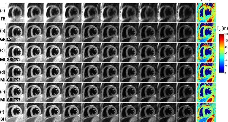
Fig. 1. Example myocardial T2 quantification image series (effective echo times TE ranging from 10 to 80 ms) and resulting T2 map obtained from free-breathing experiments: uncorrected (a); with conventional GRICS reconstruction, i.e. independent reconstruction of each image (b); with MI-GRICS1 reconstruction, i.e. GRICS with a shared motion model (c); with MI-GRICS2 reconstruction, i.e. joint reconstruction of all images and a motion model (d); with MI-GRICS3, i.e. joint reconstruction of all images, intra- and inter-image motion (e). The breath-held reference images and T2 maps are shown in (f) (the noise region including blood has been masked out).

FB

GRICS

MI-GRICS1

MI-GRICS2

T

2

[ms]

T

₂

map

TE=10ms TE=15ms TE=20ms TE=30ms TE=40ms TE=50ms TE=55ms TE=60ms TE=70ms TE=80ms

(a)

(b)

(c)

(d)

(e)

BH

(f)

MI-GRICS3

TABLEI

MAXIMAL ERROR INTRODUCED IN THE IMAGE WHEN TWO TRANSFORMATIONS ARE COMMUTED

Patient Average of all

patients

1 2 3 4 5 6 7 8 9

Maximal displacement amplitude [mm]

Motion model |U(1)_max| _39.1 _10.2 _25.6 _30.7 _22.2 _28.0 _22.4 _28.8 _44.0 _27.9 Inter-image registration

|U(2)max| 10.6 6.4 14.8 10.0 7.5 8.7 9.8 15.0 20.9 11.5

NRMSE( U(1)_{max , U}(2)_{max )}a _0.11 _0.07 _0.17 _0.15 _0.07 _0.09 _0.08 _0.10 _0.14 _0.11 NRMSE( U(1)_{max/2, U}(2)_{max /2 )} _0.04 _0.03 _0.08 _0.05 _0.03 _0.04 _0.03 _0.03 _0.05 _0.04 NRMSE( U(1)_{max/4, U}(2)_{max /4 )} _0.01 _0.01 _0.03 _0.02 _0.01 _0.01 _0.01 _0.01 _0.02 _0.01

a_NRMSE(U(1)_,U(2)_{): normalized root mean squared error introduced in the image when applying 𝑇}

𝑈(1)𝑇_𝑈(2) or 𝑇_𝑈(2)𝑇_𝑈(1).

(8)

B. Intra-image motion correction

The visual assessment of the reconstructed images shows a drastic reduction in image artifacts with all tested reconstruction (GRICS, GRICS1, GRICS2 and MI-GRICS3) compared to the uncorrected free-breathing images as can be seen in Fig. 1. Differences between the different

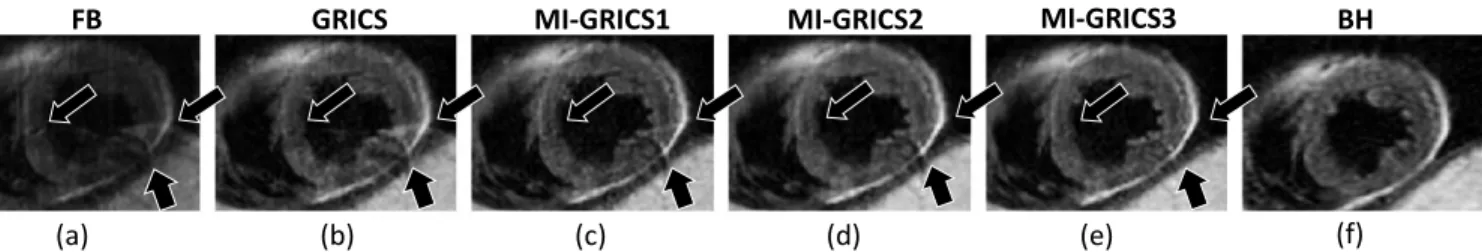
reconstructions can be observed in a typical example illustrated in Fig. 2. It can be seen that the conventional GRICS reconstruction shows residual artifacts (annotated by the arrows) which are reduced with MI-GRICS1 and further reduced with MC-GRICS2 and MC-GRICS3.

The image quality metric 𝑄𝑖𝑛𝑡𝑟𝑎 obtained with the three reconstructions are summarized in Fig. 3 and confirm the visual assessment. The improvement with this metric from MI-GRICS1 to MI-GRICS2 was statistically significant (p=0.02).

C. Inter-image motion correction

The effect of the inter-image motion correction (misalignments) is illustrated in Fig. 4. The average gradient maps over the echo times show that the spatial gradients are more spread out in the GRICS images than in the MI-GRICS1 images; there is also an improvement from GRICS1 to MI-GRICS2 and from MI-MI-GRICS2 to MI-GRICS3. The quality of the registration seemed to be similar between MI-GRICS3 and the reference (registered) breath-held images.

The inter-image motion correction quality objective scores, as assessed by 𝑄_{𝑖𝑛𝑡𝑒𝑟}, are given in Fig. 5 and are in good agreement with the visual observations. The improvement from GRICS to MI-GRICS1 was statistically significant (p=0.004); the improvement from MI-GRICS2 to MI-GRICS3 was significant as well (p=0.004).

Fig. 2. Comparison of the image quality in patient 2 (image at TEeff=70 ms) obtained from free-breathing data, including uncorrected (a), GRICS (b), MI-GRICS1 (c),MI-GRICS2 (d) and MI-GRICS3 (e) correction, with the breath-held reference data (f). Noticeable ghosting artifacts in the uncorrected image are annotated by the arrows. A gradual improvement can be observed in these areas from (b) to (e) illustrating the benefit of the joint reconstruction framework in terms of reducing ghosting/blurring artifacts.

FB GRICS MI-GRICS1 MI-GRICS2 BH

(a) (b) (c) (d) (e) (f)

MI-GRICS3

Fig. 3. Quality of the intra-image motion correction, as assessed by the gradient entropy of the reconstructed images, obtained with the proposed reconstructions. The improvement from MI-GRICS1 to MI-GRICS2 was statistically significant.

GRICS MI-GRICS1 MI-GRICS2 p=0.02* p=0.57 Qintra (unitless) MI-GRICS3 p=0.73

Fig. 4. Illustration of the inter-image motion correction efficiency. Reconstructed images from patient 3 (image at TEeff=20 ms) are shown: uncorrected (a), GRICS (b), MI-GRICS1 (c), MI-GRICS2 (d), MI-GRICS3 (e), and breath-held reference image (f). The spatial gradient images, averaged over the 10 echo times, are shown for the uncorrected (g), GRICS (h), MI-GRICS1 (i), MI-GRICS2 (j), MI-GRICS3 (k) and registered breath-held reference (l) images. The benefit of the joint reconstruction framework for inter-image motion correction is observed visually by the decreased blurring in the averaged gradient images near the endocardial and epicardial borders and in the papillary muscles (numerical results are shown in Fig.5). MI-GRICS3 seemed to perform as well as the registered breath-held images.

FB GRICS MI-GRICS1 MI-GRICS2 BH

(a) (b) (c) (d) (e)

(g) (h) (i) (k) (k)

(f)

(l)

(9)

D. Quantitative T2 analysis

T2 quantification results are summarized in Table II. The

segment-wise analysis showed that T2 values obtained with all

reconstructions are close to the reference values. For all reconstructions, differences in T2 values were not statistically

significant. Considering the quality of the T2 fit, the number of

myocardial segments that were able to be processed with good confidence (exponential fit with R2>0.97) was gradually increased from uncorrected (12), to GRICS (18), MI-GRICS1 (23), MI-GRICS2 (24) and MI-GRICS3 (27) and approached the reference breath-hold technique (29). T2 values in those

segments only were also close to the reference values and no statistical difference was observed.

The diagnostic accuracy of T2 quantification with

MI-GRICS3 is presented in Table III. Among the seven patients, three were suspected of allograft rejection due to abnormally elevated T2. The proposed technique (MI-GRICS3) agreed

with the reference technique (breath-hold) in all seven patients regarding the final diagnosis (suspicion of allograft rejection or not).

V. DISCUSSION

A framework has been proposed for the joint reconstruction of multiple images and motion and has been applied to free-breathing myocardial T2 quantification in heart transplant

patients. Our results show that the joint reconstruction of multiple images and motion (MI-GRICS1, MI-GRICS2 and MI-GRICS3) has a benefit over the joint reconstruction of a single image and motion (GRICS). Specifically, the analysis of the intra- and inter-image motion correction metrics revealed the following significant improvements: (i) the sharing of the motion model improved inter-image correction over conventional GRICS (improved 𝑄_{𝑖𝑛𝑡𝑒𝑟}) which might be explained by a more stable fit of the motion model due to dimensionality reduction; (ii) the joint image regularization improved intra-image correction (improved 𝑄𝑖𝑛𝑡𝑟𝑎) which might be explained by the more stable image reconstruction step; (iii) the added image registration improved inter-image correction further (improved 𝑄𝑖𝑛𝑡𝑒𝑟). The latter improvement was implemented with a limited extra computational cost of 13% compared to MI-GRICS2, including 9% for the registration steps alone. This was possible due to the commutation assumption described in Appendix 3 and we have checked that this assumption did not introduce large errors in our acquisition model, even in the worst case motion amplitudes. It should be noted that MI-GRICS3 is different from applying MI-GRICS2 followed by registration. This is because the inter-image motion fields ensure that the images are optimally aligned when applying

Fig. 5. Quality of the inter-image motion correction, as assessed by a metric based on normalized mutual information, obtained with the proposed reconstructions. The improvement from GRICS to MI-GRICS1, as well as the improvement from MI-GRICS2 to MI-GRICS3, were statistically significant.

GRICS MI-GRICS1 MI-GRICS2

p=0.004* p=0.004* Q_inter (unitless) MI-GRICS3 p=0.36 TABLEIII

DIAGNOSIS OF ALLOGRAFT REJECTION BASED ON T2 QUANTIFICATION

Patient number Breath-hold Free-breathing (MI-GRICS3) Agreement on diagnosis? Myocardial T2† (ms) Suspicion of rejection?‡ Myocardial T2† (ms) Suspicion of rejection?‡

1 78 ± 5 Yes 80 ± 5 Yes Yes

2 69 ± 7 Yes 69 ± 4 Yes Yes

3 61 ± 3 No 59 ± 3 No Yes

4 69 ± 4 Yes 65 ± 4 Yes Yes

5 48 ± 3 No 55 ± 7 No Yes

6 61 ± 9 No 48 ± 12 No Yes

7 52 ± 4 No 60 ± 4 No Yes

†

Myocardial T2 is the range of segment-wise T2 values expressed as mean ± standard deviation

‡

The threshold for suspicion of allograft rejection in our institution is T2>62ms TABLEII

MYOCARDIAL T2 QUANTIFICATION RESULTS FROM 7 HEART TRANSPLANT PATIENTS (42 MYOCARDIAL SEGMENTS IN TOTAL)

Uncorrected GRICS MI-GRICS1 MI-GRICS2 MI-GRICS3 _{(reference for T}Breath-hold 2) T2 in ms (all myocardial segments) 64.9 ± 13.2 (p=0.50) 62.6 ± 11.1 (p=0.66) 62.8 ± 12.1 (p=0.73) 62.4 ± 11.8 (p=0.46) 62.5 ± 11.1 (p=0.49) 62.2 ± 11.2 Number of segments with good

T2 fit (R2>0.97) 12 18 23 24 27 29 T2 in ms (segments with good fit)† 64.1 ± 11.7 (p=0.97) 62.5 ± 10.8 (p=0.44) 62.9 ± 11.8 (p=0.43) 62.6 ± 11.4 (p=0.24) 63.0 ± 11.2 (p=0.32) 64.2 ± 9.9 †

Statics performed on myocardial segments where a good fit was found with either the breath-hold or the tested reconstruction, i.e. segments such that R2 (breath-hold)>0.97 or R2_{(reconstruction)>0.97.}

(10)

the multi-image regularizer. In our results, although this did not translate into a statistically significant improvement of the gradient entropy metric, a reduction of the artifacts was visible in some cases as shown in Fig. 2.

The results also show the feasibility of using the technique for myocardial T2 quantification in heart transplant patients.

Motion-compensation strategies have been proposed previously for such applications but have been restricted to the registration of relatively low-resolution single-shot images [11], [14]. The proposed method should be particularly useful in patients who have difficulties holding their breath repeatedly and when lengthy high-resolution (multi-shot) images are desired. Another benefit is that the images generated by the reconstruction are already registered and are readily available for segmentation. Importantly segment-wise myocardial T2 values were found to be in good agreement

with the reference breath-held images. The bias (62.5 ms for MI-GRICS3 against 62.2 ms for the reference) was small compared to the inter-observer variability of T2 measurement

with this technique which was evaluated to be 2.7 ms in Ref [19]. The diagnosis with MI-GRICS3 was in agreement with that of the reference protocol in all seven patients. The acquisition time was nearly the same for the free-breathing and for the breath-held protocols although the k-space size was increased in the free-breathing experiments (from 160 to 256 in the phase encoding dimension). This was possible because the breath-held protocol comprises many idle periods so that the patient can rest between successive apneas, unlike the free-breathing protocol. Finally the reconstruction time for a T2 dataset was 9 min which is close to the scan time, making

the technique useable clinically.

In this study we used a generally applicable constraint to take advantage of anatomical redundancies in the images based on the spatial gradients (i.e. gradient co-occurrence constraint). Other redundancy constraints would be of interest, in particular those based on joint statistics of the images such as the joint entropy or the mutual information [3]. As an alternative in specific applications it might be possible to impose an analytical MR signal model [25], [26] (exponential models for T2 or T1 mapping, pharmacokinetic models for

perfusion imaging etc…), mathematical models such as B-splines [27], low-rank signal evolution models [28]–[30], or sparsity constraints in other domains such as the x-f space [31]–[33] or x-p space with p the varying acquisition parameter space [34]. Other models based on the singular value decomposition have also been proposed recently for accelerated parameter mappings [35]. Here the multi-image reconstruction framework was applied to multi-contrast MRI datasets. It might also be adapted to dynamic imaging (with or without significant contrast changes) such as perfusion imaging or cardiac cine imaging and is therefore conceptually close to the recent work in [36]. Another possible use of the framework would be in the context of multi-modal imaging. Finally other motion sensors might be used as surrogates of (or in combination with) the external sensors used here. In particular, partial MRI data (navigators or self-gated approaches) [37], [38] might give signals better correlated with the motion of organs and improve the results further.

The joint reconstruction of image and motion, as defined in Eqs. (1, 4, 7), is a non-convex optimization procedure. The

proposed approach relies on a multi-scale implementation and a linearization with respect to the motion parameters (Appendix 2). The latter step involved the optic flow equation which is known to be ill-posed (one equation with two unknowns, known as the aperture problem). Occlusions are also known to render motion estimation difficult. Here occlusions might result from large motion as structures move in and out of the imaging plane. This might cause the algorithms to be trapped in a local minimum. When applied in 2D, the method may fail when the slice thickness is small compared to the through-plane motion. In practice the clinical slice thicknesses of 8-10 mm used in cardiac MRI generally give good results. Otherwise the method might be applied in 3D to resolve through-plane motion.

One limitation of the method is the choice of the registration technique which might not be suitable for all applications. The use of a mutual information based similarity criterion might improve the registration step in Algorithm 2 slightly. More sophisticated techniques might still be necessary in case of complex contrast changes from one image to another, as can occur for instance in first-pass perfusion imaging. Another limitation of this study is the small patient population.

In conclusion we have presented a joint optimization technique that allows reconstructing N images together with both intra-image and inter-image motion models. The method allows taking advantage of anatomical redundancies in the image dataset despite the complex organ deformations during the acquisition. The feasibility of the technique was demonstrated with free-breathing myocardial T2 quantification

in heart transplant patients providing equivalent diagnostic outcome compared to the reference technique.

APPENDIX 1

FORWARD MODEL OF MRI ACQUISITION IN THE PRESENCE OF PATIENT MOTION

The forward model of the MRI acquisition process in the presence of motion is described by the following block matrix:

𝐸 = [ 𝜉𝑡₁𝐹𝐶1𝑇(𝑢𝑡₁) ⋮ 𝜉𝑡𝑁𝐹𝐶1𝑇(𝑢𝑡𝑁) ⋮ 𝜉𝑡1𝐹𝐶𝑁𝑐𝑇(𝑢𝑡1) ⋮ 𝜉𝑡𝑁𝐹𝐶𝑁𝑐𝑇(𝑢𝑡𝑁)] , (A1)

where the acquisition has been split into 𝑁 motion states 𝑡1… 𝑡N and 𝑁𝑐 parallel receiver coils. Each motion state 𝑡n is described by a dense displacement vector field 𝑢_𝑡_𝑁associated with a spatial transformation matrix 𝑇(𝑢𝑡_𝑛) (sparse matrix of size 𝑁_𝜌× 𝑁_𝜌) warping an image from the reference motion state to the 𝑛th motion state. 𝑇(𝑢𝑡_𝑛) are interpolation operators; if a linear interpolation kernel is chosen, it has 2𝑁𝑑_{elements per row (i.e. 4 in 2D and 8 in 3D). The}_𝜉_𝑡

𝑛

matrices are sparse and describe the sampling of k-space data during the 𝑛th_{motion state. 𝐹 is the Fourier transform operator}

(11)

weightings (diagonal matrices of size 𝑁_𝜌× 𝑁_𝜌) of the 𝑁_𝑐 receiver coils.

In order to reduce the complexity of the problem the number of motion states is reduced based on a clustering of the motion sensor signal values so that k-space data acquired in similar motion states are grouped into a single motion state. Further implementation details can be found in Ref [5].

APPENDIX II

JACOBIAN MATRIX DESCRIBING THE PROPAGATION OF SMALL ERRORS IN THE MOTION MODEL

The Jacobian of the data fidelity term in Eq. (3) needs to be computed with respect to 𝛼 in order to solve this nonlinear least squares optimization problem. The Jacobian describes the effect of a small perturbation 𝛿𝛼 of the motion model. Recalling the optic flow equation (given an image 𝐼, 𝐼(𝑢 + 𝛿𝑢) − 𝐼(𝑢) = 𝛻𝐼𝑇_{∙ 𝛿𝑢), the Jacobian is written and expanded} below:

APPENDIX III

INTEGRATION OF RESIDUAL INTER-IMAGE WARPING IN THE JOINT RECONSTRUCTION FRAMEWORK

Residual inter-image motion fields are estimated by registration of the reconstructed images 𝜌̃𝑖 so that the registered images are given by 𝜌_𝑖= 𝑇(𝑢̃_𝑖)𝜌̃_𝑖. In order to integrate this residual motion in the forward acquisition model, 𝑇(𝑢̃𝑖)−1 should be applied after the estimate (𝛼, 𝑠𝑖) is applied to the unknown solution image. The new forward acquisition model 𝐸̃𝑖 is accurately written as:

𝐸̃𝑖𝜌𝑖= [ 𝜉𝑖,𝑡1𝐹𝐶1𝑇(𝑢̃𝑖)−1𝑇(𝛼, 𝑠𝑡1) ⋮ 𝜉𝑖,𝑡_𝑁𝐹𝐶1𝑇(𝑢̃𝑖)−1𝑇(𝛼, 𝑠𝑡_𝑁) ⋮ 𝜉𝑖,𝑡1𝐹𝐶𝑁𝑐𝑇(𝑢̃𝑖)−1𝑇(𝛼, 𝑠𝑡1) ⋮ 𝜉𝑖,𝑡𝑁𝐹𝐶𝑁𝑐𝑇(𝑢̃𝑖)−1𝑇(𝛼, 𝑠𝑡𝑁)] 𝜌𝑖 (A3)

Here we propose to simplify (A3). Under the assumption that 𝑢̃_𝑖 is small and 𝛼 is sufficiently smooth, the two successive transformation operators can be commuted. Indeed, if 𝑣 and 𝑤 are two displacement fields and 𝜌 an image, for 𝑣 small, using the optic flow equation we have:

{

𝑇(𝑣)(𝑇(𝑤)𝜌) ≃ 𝑇(𝑤)𝜌 + ∇(𝑇(𝑤)𝜌)𝑇_{⋅ 𝑣} 𝑇(𝑤)(𝑇(𝑣)𝜌) ≃ 𝑇(𝑤)(𝜌 + ∇𝜌𝑇_{⋅ 𝑣)} = 𝑇(𝑤)𝜌 + 𝑇(𝑤)(∇𝜌𝑇_{⋅ 𝑣)}

(A4)

Furthermore if the Jacobian of 𝑤 is close to 1 (which is true for w sufficiently smooth), ∇(𝑇(𝑤)𝜌) ≃ 𝑇(𝑤)∇𝜌 and therefore 𝑇(𝑣)𝑇(𝑤) ≃ 𝑇(𝑤)𝑇(𝑣).

Finally, under the assumption that the transformations can be commuted (this assumption is termed commutation assumption in the remainder of the paper), the residual inter-image motion operators can be split away from the acquisition matrix:

𝐸̃𝑖𝜌𝑖≃ 𝐸𝑖𝑇(𝑢̃𝑖)−1𝜌𝑖= 𝐸𝑖𝜌̃𝑖 (A5) Using the intermediate variables 𝜌̃𝑖 for the optimization (instead of 𝜌_𝑖), the inter-image motion correction can be incorporated with a simple change of the regularization term as described in Eq. (7). This implementation was chosen because: (i) it was found to be more stable than introducing an additional motion operator in the forward model, which was found to lead to faster convergence and (ii) it saves computation time since the additional operators only need to be applied in the regularization step.

REFERENCES

[1] J. P. Haldar, V. J. Wedeen, M. Nezamzadeh, G. Dai, M. W. Weiner, N. Schuff, and Z.-P. Liang, “Improved diffusion imaging through SNR-enhancing joint reconstruction,” Magn. Reson. Med., vol. 69, no. 1, pp. 277–289, 2013.

[2] B. Bilgic, V. K. Goyal, and E. Adalsteinsson, “Multi‐ contrast reconstruction with Bayesian compressed sensing,” Magn. Reson. Med., vol. 66, no. 6, pp. 1601– 1615, Dec. 2011.

[3] S. Somayajula, C. Panagiotou, A. Rangarajan, Q. Li, S. R. Arridge, and R. M. Leahy, “PET Image

Reconstruction Using Information Theoretic

Anatomical Priors,” IEEE Trans. Med. Imaging, vol. 30, no. 3, pp. 537–549, Mar. 2011.

[4] F. Knoll, T. Koesters, R. Otazo, T. Block, L. Feng, K. Vunckx, F. Boada, and D. K. Sodickson, “Simultaneous MR-PET Reconstruction using Multi Sensor

Compressed Sensing and Joint Sparsity,” in 𝐽(𝛼, 𝑠, 𝜌)𝛿𝛼 = 𝐸(𝛼 + 𝛿𝛼)𝜌 − 𝐸(𝛼)𝜌 = [ 𝜉𝑡1𝐹𝐶1(𝑇(𝛼 + 𝛿𝛼, 𝑠𝑡1)𝜌 − 𝑇(𝛼, 𝑠𝑡1)𝜌) ⋮ 𝜉𝑡_𝑁𝐹𝐶1(𝑇(𝛼 + 𝛿𝛼, 𝑠𝑡_𝑁)𝜌 − 𝑇(𝛼, 𝑠𝑡_𝑁)𝜌) ⋮ 𝜉𝑡₁𝐹𝐶𝑁_𝑐(𝑇(𝛼 + 𝛿𝛼, 𝑠𝑡₁)𝜌 − 𝑇(𝛼, 𝑠𝑡₁)𝜌) ⋮ 𝜉𝑡_𝑁𝐹𝐶𝑁_𝑐(𝑇(𝛼 + 𝛿𝛼, 𝑠𝑡_𝑁)𝜌 − 𝑇(𝛼, 𝑠𝑡_𝑁)𝜌)] = ∑ [ 𝜉𝑡1𝐹𝐶1s𝑘(t1)∇(𝑇(𝛼, 𝑠𝑡1)ρ) 𝑇 ⋮ 𝜉𝑡𝑁𝐹𝐶1s𝑘(t𝑁)∇(𝑇(𝛼, 𝑠𝑡𝑁)ρ) 𝑇 ⋮ 𝜉𝑡1𝐹𝐶𝑁𝑐s𝑘(t1)∇(𝑇(𝛼, 𝑠𝑡1)ρ) 𝑇 ⋮ 𝜉𝑡_𝑁𝐹𝐶𝑁_𝑐s𝑘(t𝑁)∇(𝑇(𝛼, 𝑠𝑡_𝑁)ρ) 𝑇 ] 𝛿𝛼𝑘. 𝑁_𝑠 𝑘=1 (A2)

(12)

Proceedings 22nd Scientific Meeting, International Society for Magnetic Resonance in Medicine, Milan,

2014.

[5] F. Odille, P.-A. Vuissoz, P.-Y. Marie, and J. Felblinger, “Generalized reconstruction by inversion of coupled systems (GRICS) applied to free-breathing MRI.,”

Magn Reson Med, vol. 60, no. 1, pp. 146–157, Jul.

2008.

[6] J. Hinkle, M. Szegedi, B. Wang, B. Salter, and S. Joshi, “4D CT image reconstruction with diffeomorphic motion model,” Med. Image Anal., vol. 16, no. 6, pp. 1307–1316, Aug. 2012.

[7] P. Y. Marie, M. Angioı̈, J. P. Carteaux, J. M. Escanye, S. Mattei, K. Tzvetanov, O. Claudon, N. Hassan, N. Danchin, G. Karcher, A. Bertrand, P. M. Walker, and J. P. Villemot, “Detection and prediction of acute heart transplant rejection with the myocardial T2

determination provided by a black-blood magnetic resonance imaging sequence,” J. Am. Coll. Cardiol., vol. 37, no. 3, pp. 825–831, Mar. 2001.

[8] A. A. Usman, K. Taimen, M. Wasielewski, J. McDonald, S. Shah, S. Giri, W. Cotts, E. McGee, R. Gordon, J. D. Collins, M. Markl, and J. C. Carr, “Cardiac Magnetic Resonance T2 Mapping in the Monitoring and Follow-up of Acute Cardiac Transplant Rejection A Pilot Study,” Circ. Cardiovasc. Imaging, vol. 5, no. 6, pp. 782–790, Jan. 2012.

[9] L. Bonnemains, T. Villemin, J.-M. Escanye, G. Hossu, F. Odille, F. Vanhuyse, J. Felblinger, and P.-Y. Marie, “Diagnostic and prognostic value of MRI T2

quantification in heart transplant patients,” Transpl. Int., vol. 27, no. 1, pp. 69–76, Jan. 2014.

[10] S. Giri, Y.-C. Chung, A. Merchant, G. Mihai, S. Rajagopalan, S. V. Raman, and O. P. Simonetti, “T2 quantification for improved detection of myocardial edema,” J. Cardiovasc. Magn. Reson., vol. 11, no. 1, p. 56, Dec. 2009.

[11] S. Giri, S. Shah, H. Xue, Y.-C. Chung, M. L. Pennell, J. Guehring, S. Zuehlsdorff, S. V. Raman, and O. P. Simonetti, “Myocardial T2 mapping with respiratory navigator and automatic nonrigid motion correction,”

Magn. Reson. Med., vol. 68, no. 5, pp. 1570–1578, Nov.

2012.

[12] M. Akçakaya, T. A. Basha, S. Weingärtner, S. Roujol, S. Berg, and R. Nezafat, “Improved quantitative myocardial T2 mapping: Impact of the fitting model,”

Magn. Reson. Med., vol. 74, no. 1, pp. 93–105, Jul.

2015.

[13] R. B. van Heeswijk, D. Piccini, H. Feliciano, R. Hullin, J. Schwitter, and M. Stuber, “Self-navigated isotropic three-dimensional cardiac T2 mapping,” Magn. Reson.

Med., vol. 73, no. 4, pp. 1549–1554, Apr. 2015.

[14] S. Roujol, T. A. Basha, S. Weingärtner, M. Akçakaya, S. Berg, W. J. Manning, and R. Nezafat, “Impact of motion correction on reproducibility and spatial variability of quantitative myocardial T2 mapping,” J.

Cardiovasc. Magn. Reson., vol. 17, no. 1, Jun. 2015.

[15] F. Odille, N. Cindea, D. Mandry, C. Pasquier, P.-A. Vuissoz, and J. Felblinger, “Generalized MRI

reconstruction including elastic physiological motion and coil sensitivity encoding.,” Magn Reson Med, vol. 59, no. 6, pp. 1401–1411, Jun. 2008.

[16] A. Menini, G. S. Slavin, J. A. Stainsby, P. Ferry, J. Felblinger, and F. Odille, “Motion correction of multi-contrast images applied to T1 and T2 quantification in cardiac MRI,” Magn. Reson. Mater. Phys. Biol. Med., vol. 28, no. 1, pp. 1–12, Mar. 2014.

[17] D. Atkinson and D. L. G. Hill, “Reconstruction after rotational motion.,” Magn Reson Med, vol. 49, no. 1, pp. 183–187, Jan. 2003.

[18] F. Odille, C. Pasquier, R. Abaecherli, P.-A. Vuissoz, G. P. Zientara, and J. Felblinger, “Noise Cancellation Signal Processing Method and Computer System for Improved Real-Time Electrocardiogram Artifact Correction during MRI Data Acquisition.,” IEEE Trans

Biomed Eng., vol. 54, pp. 630–640, Mar. 2007.

[19] F. Odille, J.-M. Escanyé, D. Atkinson, L. Bonnemains, and J. Felblinger, “Nonrigid registration improves MRI T2 quantification in heart transplant patient follow-up,”

J. Magn. Reson. Imaging, vol. 42, no. 1, pp. 168–174,

Jul. 2015.

[20] Rafael C. Gonzalez and Richard E. Woods, Digital

Image Processing. Chapter 4.2.2. Addison-Wesley,

1992.

[21] M. Wood and R. Henkelman, “Mr Image Artifacts from Periodic Motion,” Med. Phys., vol. 12, no. 2, pp. 143– 151, 1985.

[22] D. Rueckert, L. I. Sonoda, C. Hayes, D. L. Hill, M. O. Leach, and D. J. Hawkes, “Nonrigid registration using free-form deformations: application to breast MR images,” IEEE Trans. Med. Imaging, vol. 18, no. 8, pp. 712–721, Aug. 1999.

[23] C. Studholme, D. L. G. Hill, and D. J. Hawkes, “An overlap invariant entropy measure of 3D medical image alignment,” Pattern Recognit., vol. 32, no. 1, pp. 71–86, Jan. 1999.

[24] M. D. Cerqueira, N. J. Weissman, V. Dilsizian, A. K. Jacobs, S. Kaul, W. K. Laskey, D. J. Pennell, J. A. Rumberger, T. Ryan, and M. S. Verani, “Standardized myocardial segmentation and nomenclature for tomographic imaging of the heart: a statement for healthcare professionals from the Cardiac Imaging Committee of the Council on Clinical Cardiology of the American Heart Association,” Circulation, vol. 105, no. 4, pp. 539–42, Jan. 2002.

[25] T. J. Sumpf, M. Uecker, S. Boretius, and J. Frahm, “Model-based nonlinear inverse reconstruction for T2 mapping using highly undersampled spin-echo MRI,” J.

Magn. Reson. Imaging, vol. 34, no. 2, pp. 420–428,

2011.

[26] N. Dikaios, S. Arridge, V. Hamy, S. Punwani, and D. Atkinson, “Direct parametric reconstruction from undersampled (k, t)-space data in dynamic contrast enhanced MRI,” Med. Image Anal., vol. 18, no. 7, pp. 989–1001, Oct. 2014.

[27] M. Filipovic, P.-A. Vuissoz, A. Codreanu, M. Claudon, and J. Felblinger, “Motion compensated generalized reconstruction for free-breathing dynamic

(13)

enhanced MRI,” Magn. Reson. Med., vol. 65, no. 3, pp. 812–822, Mar. 2011.

[28] Z.-P. Liang, H. Jiang, C. P. Hess, and P. C. Lauterbur, “Dynamic imaging by model estimation,” Int. J.

Imaging Syst. Technol., vol. 8, no. 6, pp. 551–557,

1997.

[29] B. Zhao, J. P. Haldar, C. Brinegar, and Z.-P. Liang, “Low rank matrix recovery for real-time cardiac MRI,” in 2010 IEEE International Symposium on Biomedical

Imaging: From Nano to Macro, 2010, pp. 996–999.

[30] R. Otazo, E. Candès, and D. K. Sodickson, “Low-rank plus sparse matrix decomposition for accelerated dynamic MRI with separation of background and dynamic components,” Magn. Reson. Med., vol. 73, no. 3, pp. 1125–1136, Mar. 2015.

[31] H. Jung, J. C. Ye, and E. Y. Kim, “Improved k-t BLAST and k-t SENSE using FOCUSS.,” Phys Med

Biol, vol. 52, no. 11, pp. 3201–3226, Jun. 2007.

[32] H. Jung, K. Sung, K. S. Nayak, E. Y. Kim, and J. C. Ye, “k-t FOCUSS: a general compressed sensing framework for high resolution dynamic MRI.,” Magn Reson Med, vol. 61, no. 1, pp. 103–116, Jan. 2009.

[33] M. Usman, D. Atkinson, F. Odille, C. Kolbitsch, G. Vaillant, T. Schaeffter, P. G. Batchelor, and C. Prieto, “Motion corrected compressed sensing for free-breathing dynamic cardiac MRI,” Magn. Reson. Med., vol. 70, no. 2, pp. 504–516, Aug. 2013.

[34] M. Doneva, P. Börnert, H. Eggers, C. Stehning, J. Sénégas, and A. Mertins, “Compressed sensing reconstruction for magnetic resonance parameter mapping,” Magn. Reson. Med., vol. 64, no. 4, pp. 1114– 1120, Oct. 2010.

[35] J. V. Velikina, A. L. Alexander, and A. Samsonov, “Accelerating MR parameter mapping using sparsity-promoting regularization in parametric dimension,”

Magn. Reson. Med., vol. 70, no. 5, pp. 1263–1273,

2013.

[36] S. G. Lingala, E. DiBella, and M. Jacob, “Deformation Corrected Compressed Sensing (DC-CS): A Novel Framework for Accelerated Dynamic MRI,” IEEE

Trans. Med. Imaging, vol. 34, no. 1, pp. 72–85, Jan.

2015.

[37] J. Pang, B. Sharif, Z. Fan, X. Bi, R. Arsanjani, D. S. Berman, and D. Li, “ECG and navigator-free four-dimensional whole-heart coronary MRA for simultaneous visualization of cardiac anatomy and function,” Magn. Reson. Med., vol. 72, no. 5, pp. 1208– 1217, Nov. 2014.

[38] L. Feng, L. Axel, H. Chandarana, K. T. Block, D. K. Sodickson, and R. Otazo, “XD-GRASP: Golden-angle radial MRI with reconstruction of extra motion-state dimensions using compressed sensing,” Magn. Reson.