A coupled Eulerian/Lagrangian method for the solution of three-dimensional vortical flows

A COUPLED EULERIAN/LAGRANGIAN

METHOD FOR THE SOLUTION OF

THREE-DIMENSIONAL VORTICAL FLOWS

by

HELENE MARIE FELICI

Maturite Scientifique, Abbaye du Collbge de St. Maurice, Switzerland (1979) Ingenieur, Ecole Polytechnique F'derale de Lausanne, Switzerland (1984)

SUBMITTED TO THE DEPARTMENT OF AERONAUTICS AND ASTRONAUTICS

IN PARTIAL FULFILLMENT OF THE REQUIREMENTS FOR THE DEGREE OF

DOCTOR OF PHILOSOPHY at the

Massachusetts Institute of Technology

June 1992

@1992, Massachusetts Institute of Technology

Signature of Author

Department of Aeronautics and Astronautics May 20, 1992

Certified by

Mark Drela, Thesis Supervisor Associate Prof. of Aeronautics and Astronautics Certified by

Michael B. Giles, Thesis Committee Associate Prof. of Aeronautics and Astronautics Certified by

/ _{Alan H. Epstein, Thesis Committee}

I

i Professor of Aeronautics and Astronautics Accepted by

V

Chairman, Department Graduate Committee

Aero

OF TECHNOLOGY

,JUN

0 5 1992

A COUPLED EULERIAN/LAGRANGIAN METHOD

FOR THE SOLUTION OF THREE-DIMENSIONAL

VORTICAL FLOWS

HELENE MARIE FELICI

Submitted to the Department of Aeronautics and Astronautics on May 20, 1992

in partial fulfillment of the requirements for the degree of Doctor of Philosophy in Aeronautics and Astronautics

A coupled Eulerian/Lagrangian method is presented for the reduction of numerical diffusion observed in solutions of three-dimensional rotational flows using standard Eu-lerian finite-volume time-marching procedures. A Lagrangian particle tracking method using particle markers is added to the Eulerian time-marching procedure and provides a correction of the Eulerian solution. In turn, the Eulerian solution is used to integrate the Lagrangian state-vector along the particles trajectories. The Lagrangian correction technique does not require any a-priori information on the structure or position of the vortical regions. While the Eulerian solution ensures the conservation of mass and sets the pressure field, the particle markers, used as 'accuracy boosters', take advantage of the accurate convection description of the Lagrangian solution and enhance the vorticity and entropy capturing capabilities of standard Eulerian finite-volume methods.

The combined solution procedure is tested in several applications. The convection of a Lamb vortex in a straight channel is used as an unsteady compressible flow preservation test case. The other test cases concern steady incompressible flow calculations and include the preservation of a turbulent inlet velocity profile, the swirling flow in a pipe, the constant stagnation pressure flow and secondary flow calculations in bends. The last application deals with the external flow past a wing with emphasis on the trailing vortex solution.

The improvement due to the addition of the Lagrangian correction technique is mea-sured by comparison with analytical solutions when available or with Eulerian solutions on finer grids. The use of the combined Eulerian/Lagrangian scheme results in substan-tially lower grid resolution requirements than the standard Eulerian scheme for a given solution accuracy.

Thesis Supervisor: Mark Drela,

Acknowledgments

First of all, many thanks to my advisor, Prof. Mark Drela, for the support he provided throughout this thesis. Being exposed to his innovative and practical spirit was quite an experience. Also, I would like to thank the other members of my committee, Prof Mike B. Giles for his availibility for 'very urgent questions', Prof. Alan H. Epstein for his pertinent suggestions and constructive criticism and Prof. Anthony T. Patera for his comments.

Helpful suggestions were also provided by the readers for this thesis, Profs. Marten T. Landahl and Manuel Martinez-Sanchez.

To Prof I. L. Ryhming, who was the instigator of the move to MIT, my sincere thanks for the sound advice.

Thanks to everybody in the CFD Lab for generally creating a nice working atmo-sphere and putting up with the 'extensive' use of disk space and CPU time.

To my companion in all adventures and special person in my life, you and I both know how much your constant support contributed to this work.

Research funding for this work was provided NASA Ames Research Center with Mr. Paul Stremel as Technical Monitor, by the Office of Naval Research with Mr. James A. Fein as Technical Monitor and by the NSF PYI program. Additional funding to support my education was provided by the Swiss National Foundation for Scientific Research.

Contents

1.1 Statement of the problem . . . .

1.2 Existing approaches . . . .

1.3 Present approach . . . .

1.4 Thesis outline . . . .

2 Eulerian Governing Equations

2.1 Euler equations for compressible flow . . . .

2.2 Euler equations for incompressible flow . . . .

2.3 Non- dimensionalization ...

3.1 Lax-Wendroff algorithm ... . 3... 33

3.2 Numerical smoothing ... ... .. 40

3.3 Mesh singularity treatment ... 44

3.4 Farfield boundary conditions ... 46

3.4.1 Farfield boundary conditions for compressible flow . . . . 48

3.4.2 Farfield boundary conditions for incompressible flow . . . . 52

3.5 Wall boundary condition ... ... 59

3.6 Symmetry boundary condition ... 61

3.7 Numerical implementation on unstructured grids . ... 63

3.8 Time-step restriction ... ... . 65

3.9 Accuracy study ... 66

4 Lagrangian Governing Equations 69 4.1 Lagrange equations for compressible flow . ... 69

4.1.1 Source-term contribution in compressible flow . ... 70

4.2 Lagrange equations for incompressible flow . ... 70

4.2.1 Source-term contribution in incompressible flow ... . 71

5 Eulerian/Lagrangian Integration 73 5.1 Convection of the markers and integration of the source-terms ... 74

5.2.1 Downstream integration of trajectories .

5.2.2 Upstream integration of trajectories . . .

5.3 Positioning of the markers in the flow . . . .

.

6 Correction Procedure

6.1 Entropy correction ...

6.2 Vorticity correction ...

6.2.1- Vorticity error at cell centers . . . .

6.2.2 Distribution of vorticity error . . . .

6.3 Boundary conditions for velocity correction . . . .

6.4 Discretisation error for velocity correction . . . .

6.5 Iterative procedure for the correction of vorticity . . . .

7 Vortex Preservation Test Case

8 Preservation of a Turbulent Inlet Velocity Profile in a Pipe

9 Swirling Flow in a Pipe

9.1 Swirling flow model and solution . . . .

.

9.2 Vorticity gradient augmentation . . . .

.

9.2.1 Sources for vorticity concentration . . . .

9.2.2 Introduction of a pseudo-diffusion term . . . .

. . . . . 133 136 80 . . . . . 83 88 90 90 93 98 100 102 108 117 123 123 131

10 Constant Stagnation Pressure Flow in a 900 Bend 144

11 Secondary Flow in Bent Pipes 156

11.1 M otivation .... ... ... . . 160

11.2 Lim itations ... ... 162

11.3 Outline ... ... 164

11.4 Enayet 900 bend case ... ... 165

11.4.1 Inlet velocity profile definition . ... 167

11.4.2 Enayet case 900 bend: Eulerian and Eulerian/Lagrangian results 170 11.4.3 Law of the wall correction ... 185

11.5 GTL 900 bend case ... 191

11.5.1 GTL case 900 bend: Eulerian and Eulerian/Lagrangian results . 193 11.6 Conclusions for the secondary flow in bends . ... . 195

12 Weston Wing Case 196 13 Conclusions 213 13.1 Summary ... 213

13.2 Contributions ... ... 216

13.3 Conclusions and recommendations for future work . ... 218

A Mesh Generation

B Volume and area calculations 236

C Stability analysis 239

C.1 Primitive form of Euler equations in computational coordinates ... 239

C.1.1 Primitive form: incompressible flow . ... 241

C.1.2 Primitive form: compressible flow . ... 243

C.2 Stability .. . ... ... ... .. ... ... ... ... ... .. ... 245

C.2.1 Stability: incompressible flow ... 247

C.2.2 Stability: compressible flow ... .. 248

D Brute force location of markers 249 E Newton-Raphson procedure 250 E.1 Marker location in cell ... 250

E.2 Metrics derivatives at marker location . ... 251

F Change in Circulation Due to Diffusion 253

List of Figures

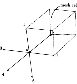
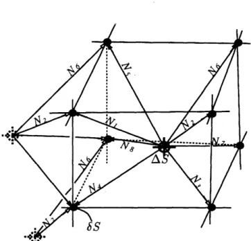
3.1 a) Mesh cells A to H surrounding node 1 and pseudo-cell P centered on node 1, b) and c) enlargement of pseudo-cell P split into eight cells Ap to Hp. Shaded surfaces indicate surfaces used for b) integration of first-order terms and c) integration of second-order terms. . ... 35

3.2 Nodal points 1 to 6 chosen for determination of fourth-difference smooth-ing at node n... .... ... 41

3.3 Mesh singularity at node 1 with pseudo-cell P. . ... 44

3.4 Exit boundary with impinging vortex. ... 57

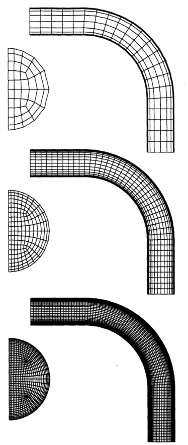
3.5 Front and side views of the grids used in the accuracy study (53 x 22 nodes, 189 x 43 nodes and 713 x 85 nodes) ... .. 67

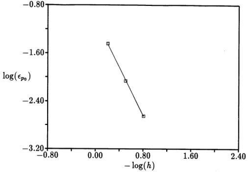
3.6 L2 norm of errors in stagnation pressure as a function of the grid spacing

for the three grid densities. ... 68

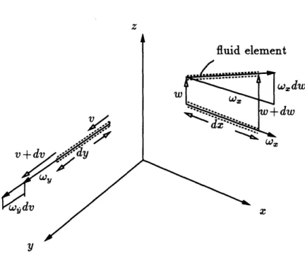
4.1 Stretching of vortex line in y direction and tilting of vortex line in x direction. ... 72

5.1 Local coordinate system in cell with node numbering and marker location at r= (X,y,z). .. ... ... ... ... ... ... ... .. ... 74 5.2 Eulerian/Lagrangian interaction procedures for downstream integration

of the trajectories: a) schematic of Eulerian/Lagrangian interaction, b

) unsteady vortex convection in contraction, c) steady swirling flow in pipe, for upstream integration of the trajectories: d ) schematic of Eule-rian/Lagrangian interaction, e) steady swirling flow in a pipe. ... . 82

5.3 Markers redistribution during downstream or upstream convection leads to a) lack of correction of the Eulerian solution, b) even correction, c) average correction in cell, and d) sparse distribution of markers in the inlet region leading to inaccurate representation of inlet flow values by the Lagrangian markers ... 85

6.1 Distribution of the error in entropy-related function AS from markers to nodes using weighted average ... 89

6.2 Local coordinate system (W*, tl*, C*) centered on nodes (represented for

the solid line marker) and vorticity error distribution from markers to cell centers. ... 92

6.3 a) Velocity correction (contribution from faces 1 4 and 6 only), and b) local coordinate system oa, 7 and local node numbering for face number 1. 94

6.4 Solid-body rotation distribution of error in vorticity to velocity components. 96

6.5 Distribution procedure ensures identical velocity correction for faces of same (area/perimeter) ratio, independently of face shape as opposed to the solid-body rotation distribution (dotted line vectors). . ... 97

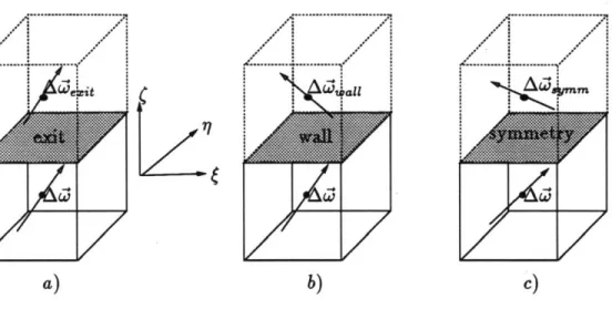
6.6 Correction in vorticity for pseudo-cells placed at a) an exit surface, b) a wall surface, and c) a symmetry surface. . ... . . 99

6.7 Contribution to velocity corrections from faces 6, 4 and 1 in the case of a) exit boundary condition, and b) wall or symmetry-plane boundary condition (additional contributions from pseudo-cells are represented as dashed line vectors) ... 101

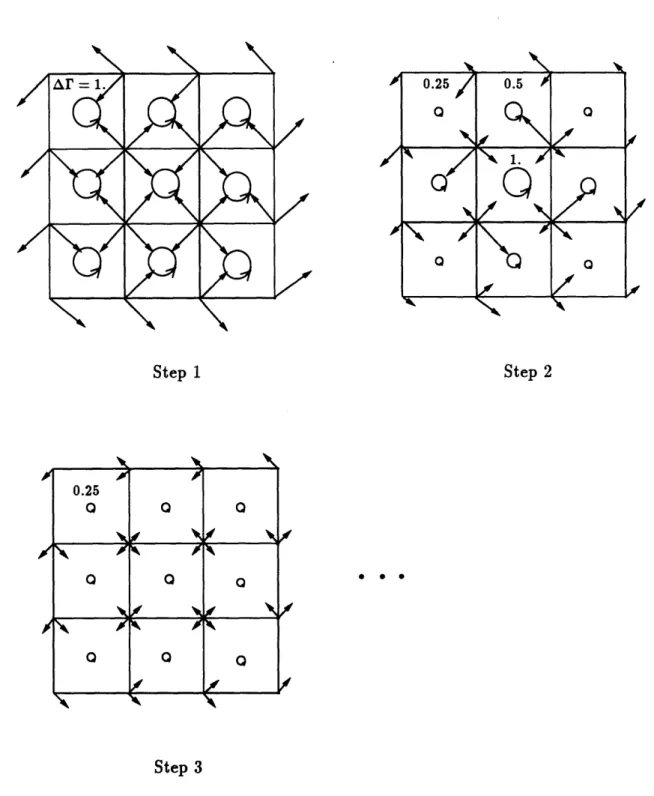
6.8 Recursive vorticity correction: error in circulation in cells and correspond-ing velocity corrections. ... 105

6.9 Convergence of recursive vorticity correction: a) maximum error in circu-lation in domain (referenced to initial error in circucircu-lation) as a function of the iteration number n and b) ratio of the maximum circulation error between two consecutive iterations. . ... .. 106

6.10 Measure of 'how slowly the iterative procedure is converging' as a function of the grid size . .. ... ... .. 107

7.1 Computational grid for vortex preservation case (129 x 17 x 9 nodes). . 109

7.2 a) Initial distribution of markers with core size and b) final distribution. 110

7.3 Pressure contours at channel mid-height, a) initial, b) final with Eulerian scheme and c) final with Eulerian/Lagrangian scheme (increment = 0.0025).113

7.4 Vorticity contours at channel mid-height, a) initial, b) final with Eulerian scheme and c) final with Eulerian/Lagrangian scheme (increment = 2.0). 113

7.5 Contours in S (entropy related function) at channel mid-height, a) ini-tial, b) final with Eulerian scheme and c) final with Eulerian/Lagrangian

scheme (increment = 0.003) ... 114

7.6 Velocity vectors at channel mid-height, a) initial, b) final with Eulerian scheme and c) final with Eulerian/Lagrangian scheme. . ... 114

7.7 Velocity profiles across vortex for exact, Eulerian and Eulerian/Lagrangian solutions. ... 115

7.8 Pressure profiles across vortex for exact, Eulerian and Eulerian/Lagrangian solutions. ... 115

7.9 Pressure coefficient as a function of the convection distance along the channel, a) Eulerian solution, b) Eulerian/Lagrangian solution and c) exact solution. ... 116

8.1 Straight circular pipe computational grid (161x25 nodes). . ... 118

8.2 Universal velocity distribution law for smooth pipes. . ... . . 120

8.3 Velocity profiles at outflow cross-section. . ... 121

9.1 Straight circular pipe computational grids: coarse grid with 125 x 25 nodes and fine grid with 384 x 49 nodes. . ... 124

9.2 Case C = 0.2: Cross-flow velocity vectors and axial vorticity on inlet cross-section for coarse grid calculations. . ... 126

9.3 Case C = 0.2: Axial vorticity contours at diverse cross-sections along the pipe, a) coarse grid Eulerian solution, b) coarse grid Eulerian/Lagrangian solution, c) fine grid Eulerian solution, d) fine grid Eulerian/Lagrangian solution (increment=0.1). ... ... .. 127

9.4 Initial and final circulation contours. . ... . 129

9.5 Case C = 0.2: Circulation on a closed curve as a function of the dis-tance along the pipe, a) coarse grid Eulerian solution, b) coarse grid Eulerian/Lagrangian solution, c)fine grid Eulerian solution, d) fine grid Eulerian/Lagrangian solution ... 130

9.6 Case C = 0.3: Axial vorticity contours at diverse cross-sections along the pipe, a) Eulerian solution on coarse grid, b) Eulerian/Lagrangian solution on coarse grid, c) Eulerian solution on fine grid, d) Eulerian/Lagrangian solution on fine grid (increment=0.1). . ... 132

9.7 Case C = 0.3: Frontal view of 3 streamlines drawn from inlet to exit of the pipe, a) Eulerian solution, b) Eulerian/Lagrangian solution (i=inlet, e=exit). . ... .. . ... ... .. ... ... . ... ... .. ... . . . . 134

9.8 Case C = 0.3: a) Front and side views of pipe with 2 streamlines, b) axial vorticity derivative bw,&/z on exit cross-section with end-points of streamlines (inc.=0.5), c) term for axial vorticity: S,, and source-term for Ow./Oz: Sa•,/az along the 2 streamlines. . ... 137

9.9 Case C = 0.6: Axial vorticity contours at diverse cross-sections along the pipe, a) Eulerian solution, b) Eulerian/Lagrangian solution, c) Eu-lerian/Lagrangian solution including Helmholtz smoothing term (incre-m ent=0.2). . ... ... ... ... 139

9.10 Estimation of the vorticity at a wall node. . ... 141

9.11 Case C = 0.6: Circulation around a closed curve, a) Eulerian solution, b) Eulerian/Lagrangian with smoothing term in the Helmholtz equation. 143

10.1 Coarse and fine grids front and side views (189 x 43 nodes and 713 x 85 nodes) with particular cross-sections. . ... . 146

10.3 Contours of z-component of vorticity at 450 station, a) Eulerian solu-tion, b) Eulerian/Lagrangian solusolu-tion, c) Eulerian solution on fine grid (increm ent = 0.05)... ... 151

10.4 Contours of streamwise vorticity at 900 station, a) Eulerian solution, b) Eulerian/Lagrangian solution, c) Eulerian solution on fine grid (incre-m ent = 0.05) .. .. .. . . . . .. . .. .. . . . .... . 151

10.5 Contours of streamwise vorticity at Id station, a) Eulerian solution, b) Eulerian/Lagrangian solution, c) Eulerian solution on fine grid (incre-ment = 0.05)... 152

10.6 Contours of streamwise vorticity at 2d station, a) Eulerian solution, b) Eulerian/Lagrangian solution, c) Eulerian solution on fine grid (incre-m ent = 0.05)... ... 152

10.7 Contours for the local error in stagnation pressure coefficient ACp₀ at 450 station, a) Eulerian solution, b) Eulerian/Lagrangian solution, c) Eulerian solution on fine grid (increment = 0.005). . ... 153

10.8 Contours for the local error in stagnation pressure coefficient ACp0 at

900 station, a) Eulerian solution, b) Eulerian/Lagrangian solution, c) Eulerian solution on fine grid (increment = 0.005). . ... 153

10.9 Contours for the local error in stagnation pressure coefficient ACp0 at ld station, a) Eulerian solution, b) Eulerian/Lagrangian solution, c) Eule-rian solution on fine grid (increment = 0.005)... ... 154

10.10Contours for the local error in stagnation pressure coefficient ACp0 at 2d station, a) Eulerian solution, b) Eulerian/Lagrangian solution, c) Eule-rian solution on fine grid (increment = 0.005) ... 154

10.11Contours in velocity norm at 450 station, a) Eulerian solution, b) Eule-rian/Lagrangian solution, c) Eulerian solution on fine grid (increment =

0.01). ...

155

10.12Contours in velocity norm at 900 station, a) Eulerian solution, b) Eule-rian/Lagrangian solution, c) Eulerian solution on fine grid (increment =

0.01). ... ... 155

11.2 Secondary flow generation by tilting and stretching of vortex lines in a

900 bend ... ... . . 158

11.3 Coarse and fine grids front and side views (320 x 36 nodes and 1223 x 71 nodes) with particular cross-sections. ... ... . . . . 166

11.4 Inlet velocity profile at grid nodes. ... .. 168

11.5 Velocity profile defined on coarse and fine grids and adjustment of the velocity profile for the fine grid case. ... . 169

11.6 Streamwise velocity contours and cross-flow velocity vectors for four sta-tions along the bend using Eulerian scheme on coarse grid. . ... . 175

11.7 Streamwise velocity contours and cross-flow velocity vectors for four sta-tions along the bend using Eulerian/Lagrangian scheme on coarse grid.. 176

11.8 Streamwise velocity contours and cross-flow velocity vectors for four sta-tions along the bend using Eulerian scheme on fine grid. . ... 177

11.9 Experimental streamwise velocity contours for four stations along the bend. 178

11.10Streamwise vorticity contours (increment = 1.0) for four stations along the bend using Eulerian scheme on coarse grid. . ... 179

11.11Streamwise vorticity contours (increment = 1.0) for four stations along the bend using Eulerian/Lagrangian scheme on coarse grid. . ... 180

11.12Streamwise vorticity contours (increment = 1.0) for four stations along the bend using Eulerian scheme on fine grid ... 181

11.13Streamlines emerging from the near wall region at the inlet of the pipe and forming the secondary flow: a) Eulerian solution, b) Eulerian/Lagrangian solution, c) Eulerian solution on fine grid. . ... 182

11.14Pressure contours on half-pipe symmetry surface (increment = 0.02): a) Eulerian solution, b) Eulerian/Lagrangian solution, c) Eulerian solution on fine grid . . . .. . . . .. . .. .. . . . .. 182

11.15Circulation around pipe cross-sections, a) Eulerian solution, b) Eule-rian/Lagrangian solution, c) Eulerian solution on fine grid. . ... 183

11.16Circulation around a closed convecting curve: a) Eulerian solution, b) Eulerian/Lagrangian solution, c) Eulerian solution on fine grid. ... 184

11.17Streamwise velocity contours and cross-flow velocity vectors for four sta-tions along the bend using Eulerian/Lagrangian scheme on coarse grid and wall correction ... ... .. 187

11.18Wall static pressure variation at four angles around the bend: a) Eulerian solution, b) Eulerian/Lagrangian solution (symbols indicate experimental values). ... ... 189

11.19Wall static pressure variation at four angles around the bend: Eule-rian/Lagrangian solution with wall velocity correction (symbols indicate

experimental values)... 190

11.20Coarse and fine grids front and side views (320 x 51 nodes and 1223 x 101 nodes) with measurement cross-section. . ... . . 192

11.21Contours of axial velocity at station located at 1.61 diameters down-stream of bend exit, a) Eulerian solution, b) Eulerian/Lagrangian solu-tion, c) Eulerian solution on fine grid, d) experiment (increment = 0.05). 194

12.1 Weston wing grid 101 x 26 x 17 nodes with C-H structure shown by 2 m esh surfaces ... ... 198

12.2 Weston wing grid detail of leading edge-tip region. . ... 199

12.3 Exit surface with clustering near trailing vortex region and symmetry mesh surface showing wake surface angle behind trailing edge. ... 199

12.4 Computed pressure coefficient on wing surface compared with experi-ments at five spanwise locations. ... 201

12.5 Initial location of markers in the trailing vortex region. ... 202

12.6 Axial vorticity in wake for stations located at 0.5 and 2.0 chords down-stream of the trailing edge, a) Eulerian solution, b) Eulerian/Lagrangian solution (inc. = 1.). ... 206

12.7 Experimental axial vorticity in wake for stations located at 0.5 and 2.0 chords downstream of the trailing edge. ... 207

12.8 Pressure coefficient in wake for stations located at 0.5 and 2.0 chords downstream of the trailing edge, a) Eulerian solution, b) Eulerian/Lagrangian solution (inc. = 0.05) ... 208

12.9 Experimental pressure coefficient in wake for stations located at 0.5 and 2.0 chords downstream of the trailing edge. . ... . . . 209

12.10Stagnation pressure coefficient in wake for stations located at 0.5 and 2.0 chords downstream of the trailing edge, a) Eulerian solution, b) Eule-rian/Lagrangian solution (inc. = 0.05). ... ... 210

12.11Experimental stagnation pressure coefficient in wake for stations located at 0.5 and 2.0 chords downstream of the trailing edge. . ... . 211

12.12Maximum axial vorticity in wake as a function of the distance behind the trailing edge, a) Eulerian solution, b) Eulerian/Lagrangian solution. .. 212

12.13Minimum pressure coefficient in wake as a function of the distance behind the trailing edge, a) Eulerian solution, b) Eulerian/Lagrangian solution. 212

A.1 Cross-sectional view of grid and distribution of cross-sections along the pipe . .. ... . .. ... ... ... ... ... ... ... .. ... .. 232

A.2 C-H mesh structure shown by different mesh surfaces. . ... . 234

A.3 Detail of wing-tip region for a streamwise cross-section located at - 50% chord with clustering in the direction perpendicular to the wall and near the tip (the derivatives are also prescribed using the source-terms). . . . 235

B.1 Dividing of cell into five tetrahedra and surface vectors numbering defi-nition . . . ... 237

Nomenclature

a Lamb vortex core radius c speed of sound

Ch airfoil chord

c2 artificial compressibility parameter C cost function

Cp pressure coefficient (Eq.12.1)

Cpo stagnation pressure coefficient (Eq.12.2) Cp1, pressure coefficient for Lamb vortex (Eq.7.6)

d pipe diameter

D2 pseudo-Laplacian operator eo total energy per unit mass F, G, H fluxes in Cartesian coordinates

J Jacobian

ho total enthalpy per unit mass p static pressure

p* reduced pressure for incompressible flows (p* = p/p) R radius

Re Reynolds number (Eq.8.1) S entropy related function (Eq.4.4)

S, projected area on the yz plane of a cell face S, projected area on the zz plane of a cell face Sz projected area on the zy plane of a cell face

t time

Ti Lagrangian source term

' position vector in Cartesian coordinates u, v, w Cartesian velocity components

ve tangential velocity u* friction velocity (Eq.8.3)

u+ velocity referenced to friction velocity (Eq.8.2) U state vector of Eulerian conservative variables Ut state vector of Lagrangian variables

Up vector of perturbed primitive variables V cell volume

V, node volume

z, y, z Cartesian coordinates

Greek:

/ pseudo-speed of sound (Eq.2.6)

ACp, local error in stagnation pressure (Eq.3.75)

Epo L2 norm of errors in stagnation pressure (Eq.3.74)

7 ratio of specific heats

r

circulation

v kinematic viscosity

V2 second-difference numerical smoothing coefficient v4 fourth-difference numerical smoothing coefficient VI Lagrangian pseudo-diffusion coefficient

p static density At time-step

7P grid weight function

I vector of linearized characteristic variables W vorticity vector

7,

il, ( local coordinates

Superscripts: n time index Subscripts: c corrected quantity e Eulerian quantity kc cell averaged in, out inlet, outlet

i, n node index

1 Lagrangian quantity maz maximum quantity min minimum quantity

p predicted quantity z, y, z z, y, z components

0 total (stagnation) conditions oo freestream conditions

Accents:

Chapter 1

Introduction

1.1

Statement of the problem

Over the last few years, the improvement in CPU and memory capabilities of modern supercomputers has rendered practical the solution of flow problems of more and more complex nature. However, the efficient numerical treatment of flow non-homogeneities, such as vortex wakes or tip vortex roll-up, embedded in an otherwise smooth background flow field remains a challenging field of study. In many practical applications, the prediction of the strength and the position of the vortical regions reveals to be of primary importance. For instance, the flow around an helicopter rotor blade presents a case of strong interaction between the shed vortices due to one blade and the following blade. The prediction of the resulting load variations requires the accurate solution of the shed vortices, of their trajectories and of the subsequent interaction phenomenon. Another example is the prediction of the secondary flow through a bend with a pump attached at the bend exit. The location and strength of the secondary vortex, created by the tilting and stretching of the inlet boundary-layer vorticity, must be solved accurately, as a possible noise source and a performance loss may result from the impingement of the secondary vortex on the rotating blades.

Vortex-sheets, secondary flows, or vortex roll-up phenomena are all characterized by transverse length scales differing by orders of magnitude from the length scale of

the supporting flow field (the transverse length scale of trailing vortices has been found experimentally to be as low as 5% of the airfoil chord [57]). Since the solution of these vortical features has often to cover a convection length much higher than their intrinsic length scale, the global prediction of vortex-dominated flows proves to be highly sensitive to small local errors. This makes these flow features difficult to be captured by finite-difference methods.

1.2

Existing approaches

Incompressible vortex methods and potential methods with fitted vortex sheets are not susceptible to the numerical diffusion. Examples of incompressible vortex methods, using Biot-Savart law to compute the velocity field, include the method used by Leonard [41] where the flow vorticity is modeled as a collection of a few isolated vortex-tubes with a computational element assigned to each vortex tube and Knio's study [38] where a three-dimensional vortex scheme is based on the transport of vorticity and material elements. Additionally, gradients of the scalar field are transported and the scalar field itself is recovered using Biot-Savart law.

Potential methods presuppose some a priori knowledge (either from a known solution or from empirical data) on the vortex structure or position, since potential methods do not 'capture' embedded vorticity as part of the solution. This limitation becomes especially acute when solving complex flow problems where an a priori information is not always available. Scully [64] and Miller [44] have used a Biot-Savart formulation for an incompressible flow solution of an helicopter rotor wake. Hassan [25] used the Euler equations in an implicit scheme and modeled the blade-vortex interaction by computing the vortex-induced velocities following Biot-Savart law. Steinhoff [71, 72] presented an alternative method for an aircraft configuration, where the strength, position and shape of the vortex sheet were calculated as part of the solution. The internal structure of the wake was, however, still to be specified. Ramachandran [54] used a potential method

with embedded vortex wakes for the compressible flow solution of a rotor wake. The body was included in the calculation similarly as the rotor wake as a vorticity sheet

whose strength is determined iteratively.

The use of an Euler or a Navier-Stokes solver presents the advantage that the em-bedded vorticity is captured as part of the solution. Poor solution representation is, however, a common feature of Eulerian and Navier-Stokes solvers in regions of high gra-dients. More precisely, the errors introduced by discretizing the equations of motion can be expressed in terms of dissipation and dispersion phenomena. In addition, rounding errors are introduced randomly in the solution. The dissipation expresses the fact that the finite difference model loses energy as the time progresses. Because numerical dis-sipation can be advantageous by counteracting unwanted instabilities and oscillations (for example saw-tooth modes), it is added to non-dissipative formulae. The disper-sion errors correspond to the decay of a wave form into separate spurious oscillations and always occur with finite-difference formulae since their dispersion relation is always non-linear.

Because most common second-order accurate finite-difference schemes will smear and distort regions of high gradients, corresponding grid clustering seems the obvious approach. However, depending on the flow topology, this procedure could reveal to be prohibitively expensive. For example, the solution of the flow around helicopter blades involves the prediction of the interaction between the tip vortex from a blade and the following blade. Because the resulting flow presents vortex regions of high extent and is highly non-homogeneous, standard clustering of the grid would lead to high computational cost. As Drela [20] reported, a suitably overall fine grid would imply - 260 billion points for a rotor wake solution. The sensitivity of the solution to the grid coarseness has, therefore, prompted several studies.

Selective refinement of the grid is used by L5hner [42] in an adaptive algorithm in two dimensions. In three dimensions, however, the algorithm would undoubtedly present much complexity. Nakahashi [46] uses a 2-D solution adaptive structured grid

method based on variational principles and spring analogies. A multigrid solution of the Euler equations using an implicit scheme has been performed by Jameson [37] and has proven effective for CPU reduction in two-dimensional applications. The three-dimensional application would certainly prove to be more involved. Landsberg [40] has studied vortex capturing using adaptation and a three-dimensional finite-element solver. Also Schmatz [63] presented a two-dimensional zonal solution to model the weak or strong viscous/inviscid interactions in subsonic and transonic flows. Powell [49] used an adaptive mesh procedure working on an unstructured mesh for solving the conical Euler equations for leading-edge vortex flows. In this respect, unstructured grids present a strong advantage over structured grids because of the flexibility of adding new grid resolution in defined areas.

An alternative to grid refinement is to use a high-order accurate scheme, a method used by Rai [53] who presented a fifth-order upwind-biased scheme in a blade/vortex interaction problem. Steger [70] used an implicit fourth-order accurate scheme for the computation of vortex wakes. However, the advantage of using these high-order accurate schemes, with suitable clustering of points in the regions of high gradients, is still linked to grid smoothness (more difficult to obtain in three dimensions) and were demonstrated on grids prohibitively fine for complex three-dimensional applications.

Perturbation methods, instead, rely on a known' flow solution in some areas of the computational domain such as to correct the numerical diffusion encountered in the basic finite-difference flow solution. Roberts [57, 56] applied this methodology, first introduced by Chow [15] to the rotor wake and blade/vortex interaction problems by coupling the Euler equations to a free-wake model of the rotary wing wake. The main drawback here is the need for a known solution which limits the correction method to regions of simple behavior (the correction can not be performed where the vortex impinges on the airfoil for instance). In a similar approach, Srinivasan [69, 68] uses the 2-D thin-layer Navier-Stokes equations and a prescribed vortex for computing the flow

1

This is done from an analytic solution if available or from a previously computed high resolution local solution of the flow field.

over rotor blades.

The 'Cloud in Cell' technique, first introduced by Christiansen [16] and then trans-formed by Baker [5] for a 2-D incompressible inviscid fluid, uses an area averaged vor-ticity distribution from markers in cells onto grid nodes where Poisson's equation is solved. The circulation distribution must, however, be known at each marker and a three-dimensional solution is not straightforward. Also Basuki [7] used the inviscid 'Cloud in Cell' technique with vortices tracked though the grid on which the velocity is found by a finite-difference method. Poor resolution of the velocity field was, however, reported.

The advantages of spectral methods are accuracy, ease of implementation and the low number of collocation points required for a computation when compared to the

dis-cretization used in finite-difference methods. However, they lead to large matrices for more than one non-periodical direction (which is the case for the flow cases treated here) and are difficult to apply in computational domains of complex shapes. Also, no discon-tinuity (as a shock, for example) is allowed as part of the solution. Furthermore they are more time restrictive than finite-difference methods for unsteady flow calculations.

1.3

Present approach

As mentioned in the previous section, the Euler or Navier-Stokes equations present the advantage of directly capturing embedded vorticity, when compared to potential methods with fitted sheets. For example, as reported by Murman [45] and others [50, 9], the use of the Euler equations provides a good tool for a study of flows around wings enabling the study of the leading-edge vortex. The capturing capabilities of Euler or Navier-Stokes solvers are, nevertheless, limited by grid resolution issues. As an alternative to the methods dealing with this problem, this thesis presents a technique for substantially improving the capturing capabilities of time-marching Eulerian solvers.

This method does not require the knowledge of an a priori solution, grid refinement or the use of higher-order schemes.

The objective of this research is then to construct an alternative solution procedure to reduce the numerical diffusion observed in standard Eulerian time-marching calculations and to demonstrate the feasibility, efficiency and flexibility of the method by application to different flow problems. These include three-dimensional steady, unsteady, internal as well as compressible and incompressible inviscid flow cases. Furthermore, the extension of the method to include the Navier-Stokes equations (not performed in the frame of this thesis) is judged to be straightforward.

The present method consists in the addition of a Lagrangian particle tracking so-lution to a standard Eulerian soso-lution in order to enhance its vorticity and entropy capturing capabilities. This method is based on the approach of Drela [20] in two di-mensions and is here extended to include three-dimensional flow cases. The combination of the Eulerian and Lagrangian solvers takes advantage of both the accurate convection description of the Lagrangian technique and the 'elliptic' representation of the Eulerian solution which enforces the mass conservation and sets the pressure field. Briefly, the Lagrangian solution is based on particle markers carrying vorticity and entropy, and convecting with the local flow through the Eulerian grid. The Eulerian solver is used to conserve mass and to provide the source terms required for the Lagrangian time integration. In turn, since the Lagrangian solution is immune to the numerical diffu-sion process occurring in the Eulerian solver, it accurately captures the convection of vorticity and entropy. This information is then used to locally correct the Eulerian so-lution and to reduce its numerical diffusion errors. Each Lagrangian marker influences the Eulerian solution only locally (as opposed to the 'Cloud in Cell' technique where each marker has an influence on the entire flow field), which makes this scheme well suited for three-dimensional flow solutions. Also, the Lagrangian solution needs to be computed only in regions of interest as markers can be located selectively in the flow. No a priori information is required on the flow structure since the Lagrangian solution includes inherently 'convective' capabilities.

1.4

Thesis outline

Chapters 2 and 3 present the equations, numerical procedure and accuracy study for the Eulerian solver for both the compressible and incompressible flow cases. The mesh generation technique is described in Appendix A. The Lagrangian equations are the object of Chapter 4, whereas the coupling of the two solvers in the time integration is described in Chapter 5 for different flow configurations. Finally, the correction proce-dure by which the Lagrangian equations influence the Eulerian solution is presented in Chapter 6.

The first test case, discussed in Chapter 7, is the convection of a Lamb vortex in a three-dimensional uniform background flow and is used as a preservation test for a compressible unsteady flow. An analogous test case is presented in Chapter 8 as the preservation of a turbulent inlet velocity profile in a straight pipe. The swirling flow in a straight pipe is the object of Chapter 9 with an emphasis on the development of a vorticity gradient augmentation phenomenon and the particular solution adopted with the combined Eulerian/Lagrangian solver. The vorticity errors and stagnation pressure losses encountered in the Eulerian solution of a 900 bend are reduced by the use of the Lagrangian correction method in Chapter 10.

Chapter 11 deals with the secondary flow in bent pipes. The secondary flow genesis is first described and Eulerian and Eulerian/Lagrangian solutions are computed and compared with experiments. The introduction of a simple 'law of the wall' model is attempted in order to deal with viscosity effects.

The last case, reported in Chapter 12, is the external flow over a three-dimensional wing. This chapter emphasizes the spurious numerical diffusion of the tip vortex behind the trailing edge and the correction obtained using the combined Eulerian/Lagrangian scheme. Comparison with experimental data is also performed.

Chapter 2

Eulerian Governing Equations

Provided the tangential forces applied on fluid particles are small compared to the pressure forces, the fluid can be treated as inviscid. The evolution of an inviscid flow in time and space is described by the Euler equations [60, 3]. Here, these equations are used for the solution of both steady incompressible and unsteady compressible flow fields. The numerical solution procedure using a Lax-Wendroff scheme is the object of

the next chapter.

2.1

Euler equations for compressible flow

For the solution of unsteady compressible flows, the solution is marched forward in time from an initial condition. The Euler equations expressed in a (z, y, z) Cartesian coordinates system and in conservation form are

OU

OF

OG

OH

S=

O

+

y

+

_T

_(2.1)

where U, the state vector of the conservative variables and F, G, H, the fluxes of mass, momentum and energy are written as

P pu pv pw

pu pu2 _{+ p puv puw}

U= pv F= puv ,G= v2 + p ,H= pvw

pw I puw pvw pw2 + p

peo,

pu(eo + pip)

pv(eo + pip)

pw(eo + pip)

p denotes the fluid density, u, v, w are the velocity components in the Cartesian co-ordinates, p is the pressure and eo is the total energy per unit mass. Additionally the perfect gas law is used to relate the total energy per unit mass to the pressure as

P = (y - 1)p(eo -

(u + v

_{+ w}

_)),

_(2.2)

c = -, ho = eo +-. (2.3)

P P

2.2

Euler equations for incompressible flow

For an incompressible unsteady flow, the state vector U and the fluxes F, G and H are written as

0

U

v

w

U=

F=

G=

H=

,(2.4)

uv

The main problem in solving the Euler equations for an incompressible flow is to link the velocity changes to the pressure changes in a way that enforces the divergence-free

condition. In two dimensions, the solution of steady or unsteady incompressible flows can be achieved through the stream function-vorticity formulation (therefore eliminating the pressure from the governing equations). In three-dimensional flow calculations, however, this solution technique becomes more complex and other solution procedures are usually sought. The vorticity-velocity formulation used by Dennis [17] replaces the two-dimensional stream function-vorticity formulation. The Poisson's equation method developed by Harlow [24] consists of iteratively adjusting the pressure field by solving a Poisson type equation for the pressure change. Poisson's equation is obtained from the requirement that the continuity equation must be satisfied. Since this method involves an iterative procedure it is, however, very time consuming for three-dimensional applications.

A well-known class of solution procedures for steady compressible flows is the time-marching method where the full unsteady Euler equations are used and the solution evolves through a pseudo-unsteady process from an initial guess to the final steady-state. Nevertheless, in the limit of an incompressible flow, sound waves with very large speed tend to make the system stiff and render this inefficient. A well-known solution to this problem, and the method used in this work, is the artificial compressibility concept introduced by Chorin [14]. The purpose of this technique is to transform the character of the Euler equations for an incompressible flow from elliptic to hyperbolic by adding a time-dependent term in the continuity equation. This particular method has been successfully tested on an extensive set of internal and external incompressible flow problems [58, 13, 55, 61, 79].

To introduce a time-derivative of the pressure in the continuity equation, the di-vergence term is multiplied by the "artificial compressibility" parameter c2 so that the

modified state and flux vectors are defined as

p*

cu

c2V

caw

U u2

+-

v u v v2 p* WtD

w 1w u/ vw w 2

+

The value of the artificial compressibility parameter can be adjusted to increase the convergence rate of the time-marching procedure. When steady-state is reached, the modified system of equations reduces to the standard Euler equations for steady flow. Also pseudo-time stepping can be used since the unsteady process is of no interest here and only the steady-state solution is retained.

The introduction of the artificial compressibility parameter results in giving finite speed to the propagating waves, in contrast to truly incompressible flow where the waves move with an infinite speed. The pseudo-speed of sound 3 is computed in Section 3.4 by analyzing the linearized Euler equations with 1-D variations. 3 depends on the artificial compressibility parameter c2 as

/3=

u

c

.+

.

(2.6)

Chang [13] estimates the relation between the parameter ca and the rate of convergence by looking at the speed of the propagating waves. The time taken by a wave to travel from the inlet of the computational domain to the exit over a distance L and back is

L L 23L

t

+

u

-

(2.7)

This value represents the minimum time needed for convergence. If the time-step allowed for stability is At, then N the number of time-steps required becomes

N

23L 2 -( 2) 2L (2.8)

C2 At

2

At'

a decreasing function of c.. Regarding the value of the artificial compressibility param-eter, it is shown in Section 3.4 that the ratio of the largest to the smallest eigenvalues of the linearized Euler system of equations is dependent on /3. / is therefore a measure

of the condition of the system. Rizzi [55] has verified numerically that a ratio c2/u 2 between 1 and 5 ensures the system to be well-conditioned. In this particular study a constant value of c2/u2 of 1 is used.

Another advantage of the artificial compressibility method is its natural extension to the handling of the Navier-Stokes equations [13]. Also the same concept has been used for the solution of unsteady flows problems [43].

2.3

Non-dimensionalization

The Euler equations are used in a non-dimensionalized form which allows for the flow values to fall within prescribed limits. The arbitrary reference values are given below for the different flow cases treated in this work.

For the compressible flow in a channel the reference quantities are the channel length L, the inlet stagnation speed of sound co0, and the inlet stagnation density Po0i so that

the non-dimensional variables are r = z

L/coij'

PoicOCin

The corresponding reference inlet stagnation pressure and enthalpy are

(Poi Po, 1 7 (Po) 1 (2.9)

P c, 7 I 1 (Po.), - 1"

For incompressible flow in pipes, the reference quantities are the pipe radius R, and the inlet mass-flow averaged velocity ui,-. For the incompressible flow around an airfoil

the reference length has been chosen as the airfoil chord ch

is the freestream velocity Uo. If the reference length and denoted by L,,f and U,,f, then

t

Lref

/Uref'

e,

f

7r = ,

and the reference velocity the reference velocity are

z

L:;:

wr =

Chapter 3

Euler Solver: Numerical Procedure

3.1

Lax-Wendroff algorithm

The Euler solver uses a Ni-Lax-Wendroff node-based scheme on an unstructured grid. An explicit time-marching procedure subject to appropriate boundary conditions is used to drive the solution from an initial guess to a steady-state or to an unsteady solution.

The numerical procedure has been introduced by Ni [47] for two dimensions and has been described later by Ni and Bogoian [48] for a three-dimensional application on a structured grid. The present chapter deals with the algorithm description for unstructured meshes.

The spatial discretization uses hexahedral cells and the change in time of the state vector U is expressed as a function of the fluxes across the cell faces. These are evaluated as the average of the fluxes at the corner nodes. The residual (found from summing the fluxes across the six faces of each cell) is used to determine the change in the state vector and is then distributed back to the nodes following the Lax-Wendroff algorithm.

second-order terms as

U

U =At

OUv

+At

_2U

_(3.1)

Ot

2

and the time derivative of the state vector U is related to the spatial derivatives of the fluxes F, G, H by Equation (2.1)

OU

OF

OG

OH

a--:

a

ay

az"

(3.2)

Ot

OX

OYy

Oz

Hence, the change in the state vector between two iterations is

AU

= U•+ - U = At

O+y

+

At [ 0(At

(

_{(At OH)]}

2

x

at

+y

at

+ tz

at

The second-order changes are defined as

F dG AOH

AF = At OF G = At AH = At . (3.4)

t '

at '

t

Integrating over a pseudo-cell P formed by joining the centers of the cells surrounding node 1, as sketched in Figure 3.1a), gives

6UdV =

-At

(

+ y +

-

-A

AG" +

AH)]

dV.

(3.5) Then by applying Gauss' theorem we get

6U

= -

t

(F, G,H)

dS -

(AF, AG, AH) .

dS.

(3.6)

V

Jp

Jp

i' denotes the unit normal to the cell surfaces pointing outwards, V₁ is the volume of

P. At1 is the time-step associated with node 1 and is defined by

(Vi

1=

l

V

t

(3.7)

8 cells

where the sum operates over the eight cells surrounding node 1. In Figure 3.1a) node 1 is surrounded by mesh cells A, B, C, D, E, F, G, H (mesh cells D and H are not represented for clarity purposes). Figure 3.1b) and c) represent the pseudo-cell split into eight cells Ap, Bp, Cp, Dp, Ep, Fp, Gp, Hp. The integration of the first-order terms is found by

b)

Bp

B

Hp

a)

c)

Figure 3.1: a) Mesh cells A to H surrounding node 1 and pseudo-cell P centered on node 1, b) and c) enlargement of pseudo-cell P split into eight cells Ap to Hp. Shaded surfaces indicate surfaces used for b) integration of first-order terms and c) integration of second-order terms.

integrating over all the surfaces of these eight volumes as shown by the dashed surfaces of Figure 3.1b)

At

_{(F, G, H) -dS}

_A

_(F,G,H).

-dS.

V,

Fp

V

1

jA._...

Each of these integrals is estimated as one eighth of the surface integral over the corre-sponding mesh cell surrounding node 1 so that

-A (F, G, H) - dS =- A,....(F, G, H) - dS. _(3.9)

The integral of the second-order terms is performed over the ezternal surfaces of the eight cells Ap to Hp as represented by the dashed surfaces in Figure 3.1c), so that

At

(AF,AGAH)A

-,dSAA,

_A

A

_{(AF, AG, AH). -i dS. (3.10)}

2 V2V1

p

GApA,Ap2,Ap3

Hp1, Hp2, Hp3

The integral over the surface Ap1 is evaluated as one fourth of the integral over

the 'mean surface' A1 defined as the average surface between two opposite faces of mesh

cell A. The 'mean surface' a3 is represented on Figure 3.1a). A similar procedure applies for surfaces Ap2 to Hp3 so that

At

(AF, AG, AH)

dS =

(F,

_{G, AH) -n dS.}

jJp\

-

8V

8

V•

-,A2,As

6U

1

=

6U1A +

UlB... +

UH,

and so on for the contributions of cells B to H. 6U1A can then be written as

1 At1 VA

U1xA --

AV AUA

L

1 (t _A1,A2,A3

where VA is the volume of cell A. S,, S, and S_ are the components of the surface vector in the Cartesian coordinates, and AUA is the average first-order change in the state vector in cell A defined as

_AtA

_tA

df=

AUA

=

(F, G, H)

-(S,

+

GS,

+

A AVA (3.15)

and F, G,

iH

The second-order terms AFA, AGA, AHA are expressed as a function of the change AUA as

A

OF)

A OU A AGA = (G) AUAA AHA = A

However, a more straight forward way to compute the second-orders terms is to use the changes in the conservative variables as follows.

For a compressible flow

AUA =

A(pV)

A(pw)

A(pE)

A(pv)

AFA =

IA(pu)

uA(pu) + puAu + Ap uA(pv) + pvAu

uA(pw) + pwAu

u(A(pE) + Ap) + (pE + p)Au

A(pw)

wA(pu) + puAw

wA(pv) + pvAw

wA(pw) + pwAw + Ap

w(A(pE) + Ap)

+

(pE + p)Aw

(3.16)

AGA=

where UA, A, WA are obtained from averages over the nodes of cell A and

(AU)A

=

((A(PU)-- UAP)/P)A

(AV)A

=

((A(pv) - vAP)/)A

(XUW)A = ((A(PW) - WAP)/P)A

- ) (A(pE) - uA(pu) - vA(pv) - wA(pw) + A(u'2 ++ 2

/71 ₂

) A

For an incompressible flow

AUA =

AGA=

where UA, VA, WA are

ol

Ap* Au Av Aw

c2 Av

SAFA

=

c•Au

In addition to Equation (3.14), the change in the state vector at contributions from the cells B to H written as

6U1B

5Uic

6U1D

=

VD AUD

8 V AtD

node 1 receives

(AFBSz + AGBSY + AHBSz)),

B1,B2,B3

Z

(AFcS, + AGcS, + AHcSz))

(3.17)

(3.18)

D

(AFDS= +

, (3.19)

D1,D2,Ds (Ap)A 1 Ati VB

=

-

_AU

1

At,

Vc

8 V

tUc-II ,

I

VE

VAUF

VAUG

Ata

A•H

-U

- (AFES2

+ AGES,

+ AHESz),,,

EXE₂,E3

E

(AFF

S,

+ AGFSa +

S(AFGS,

+ AGGS, +

At,

8

V

8

V-E

(AFHS,

_{+ AGHSy + AHHSZ))}

HI,H 2,H3

(3.20)

(3.21)

(3.22)

.(3.23)

The calculation of the cell volumes, face areas and volumes associated with cell nodes is described in Appendix B. 6_U1E 6

_U1F

_U1H

AHFSz))

_,

3.2

Numerical smoothing

By expanding the dispersion relation of the Lax-Wendroff scheme into Taylor series, it can be seen that the Lax-Wendroff scheme carries both an inherent dissipation term and a third-order dispersion error [73, 76]. The former term accounts for the scheme stability when operating on smooth flow fields. Nevertheless, the dispersion error is responsible for the introduction of oscillatory modes in the solution. In order to damp these background oscillations, an artificial dissipation term has to be added to the Euler equations.

The compressible flow version of the Euler solver uses a standard Laplacian second-difference smoothing. The Laplacian is obtained at node 1 by summing the second-difference between the state vector at node 1, U1, and the cell-averaged state vector of the 8

surrounding cells UA to UH (the nomenclature is described in Section 3.1). The change in the state vector at node 1 is then the sum of Equation (3.13) and the contribution from the second-difference smoothing

U~1 = 6U1A - ... U1H + 2 ( kC - ) (3.24)

Skc=A,...,H

where v2 is an artificial viscosity coefficient, V1 the volume associated with node 1 and

Vkc the volume of the cell kc. At1 and Atke are the time-steps associated with the node

1 and the cell kc, respectively.

The incompressible flow version of the Lax-Wendroff algorithm uses a fourth-difference smoothing. The fourth-difference operator is constructed as a second-difference of a difference. Instead of using two standard Laplacian operators, the inner second-difference involves a "pseudo-Laplacian" operator defined by Holmes and Connell [31] and obtained at node n as

D2= i(Ui - Un), (3.25)

i=1