Coupling dry deposition to vegetation phenology in
the Community Earth System Model: Implications
for the simulation of surface O[subscript 3]
The MIT Faculty has made this article openly available.
Please share
how this access benefits you. Your story matters.
Citation
Val Martin, M., C. L. Heald, and S. R. Arnold. “ Coupling Dry
Deposition to Vegetation Phenology in the Community Earth System
Model: Implications for the Simulation of Surface O[subscript 3].”
Geophys. Res. Lett. 41, no. 8 (April 16, 2014): 2988–2996. © 2014
American Geophysical Union
As Published
http://dx.doi.org/10.1002/2014GL059651
Publisher
American Geophysical Union (AGU)
Version
Final published version
Citable link
http://hdl.handle.net/1721.1/89479
Terms of Use
Article is made available in accordance with the publisher's
policy and may be subject to US copyright law. Please refer to the
publisher's site for terms of use.
RESEARCH LETTER
10.1002/2014GL059651 Key Points:• The dry deposition scheme (Wesely, 1989) is corrected and optimized in CESM
• Dry deposition velocity and sur-face O3simulations are significantly improved
• Linking deposition to LAI is key to simulate O3responses to vegetation changes Supporting Information: • Readme • Figure S1 • Figure S2 Correspondence to: M. Val Martin, [email protected] Citation:
Val Martin, M., C. L. Heald, and S. R. Arnold (2014), Coupling dry depo-sition to vegetation phenology in the Community Earth System Model: Implications for the simulation of surface O3, Geophys. Res. Lett., 41, doi:10.1002/2014GL059651.
Received 19 FEB 2014 Accepted 1 APR 2014
Accepted article online 2 APR 2014
Coupling dry deposition to vegetation phenology
in the Community Earth System Model: Implications
for the simulation of surface O
3
M. Val Martin1, C. L. Heald2, and S. R. Arnold3
1Atmospheric Science Department, Colorado State University, Fort Collins, Colorado, USA,2Department of Civil and
Environmental Engineering, Massachusetts Institute of Technology, Cambridge, Massachusetts, USA,3Institute for Climate
and Atmospheric Science, School of Earth and Environment, University of Leeds, Leeds, UK
Abstract
Dry deposition is an important removal process controlling surface ozone. We examine the representation of this ozone loss mechanism in the Community Earth System Model. We first correct the dry deposition parameterization by coupling the leaf and stomatal vegetation resistances to the leaf area index, an omission which has adversely impacted over a decade of ozone simulations using both the Model for Ozone and Related chemical Tracers (MOZART) and Community Atmospheric Model-Chem (CAM-Chem) global models. We show that this correction increases O3dry deposition velocities over vegetated regions and improves the simulated seasonality in this loss process. This enhanced removal reduces the previously reported bias in summertime surface O3simulated over eastern U.S. and Europe. We further optimize the parameterization by scaling down the stomatal resistance used in the Community Land Model to observed values. This in turn further improves the simulation of dry deposition velocity of O3, particularly over broadleaf forested regions. The summertime surface O3bias is reduced from 30 ppb to 14 ppb over eastern U.S. and 13 ppb to 5 ppb over Europe from the standard to the optimized scheme, respectively. O3deposition processes must therefore be accurately coupled to vegetation phenology within 3-D atmospheric models, as a first step toward improving surface O3and simulating O3responses to future and past vegetation changes.1. Introduction
Surface ozone (O3) is a harmful air pollutant that is toxic to humans and ecosystems. O3concentrations in the troposphere are controlled by a balance among chemical production, stratospheric influx, and loss pro-cesses. A major loss process for O3is surface dry deposition, accounting for about 20% of the O3lost in the troposphere [Wild, 2007]. The majority of this O3removal occurs over vegetation, mainly by direct uptake through the stomatal pores of plants and by direct deposition over the leaf cuticles [e.g., Wesely, 1989]. Changes in vegetation as a result of human activities and climate change are of great concern for O3air quality [e.g., Sanderson et al., 2003; Ganzeveld et al., 2010; Wu et al., 2012]. For example, deforestation may decrease foliar uptake, prompting a rise in O3concentration. In addition, changes in vegetation affect emis-sions of O3precursors (e.g., biogenic volatile organic compounds and soil NOxemissions), which in turn affect OH, an important oxidizing agent in the atmosphere that regulates the lifetime of the greenhouse gas methane.
Surface O3is challenging to simulate in 3-D atmospheric models [e.g., Murazaki and Hess, 2006; Wu et al., 2007; Lamarque et al., 2012], due to the nonlinearity of the chemistry, the complexity of physical process, and the heterogeneity of precursor emissions. A recent well-known issue in some models is the positive bias of surface ozone of more than 10 ppb over eastern U.S. and Europe during the summer [e.g., Murazaki and Hess, 2006; Fiore et al., 2009; Reidmiller et al., 2009; Lamarque et al., 2012]. For example, Murazaki and Hess [2006] reported a very large positive bias (40–60 ppb) for the maximum daily 8 h averaged (MDA8) O3over eastern U.S. in the summer with the Model for Ozone and Related chemical Tracers version 2 (MOZART-2). Lamarque et al. [2012] reported a similar bias for the Community Earth System Model (CESM) over the eastern U.S. and a bias of 10–30 ppb over Europe. A positive bias of 10–20 ppb was reported for summer-time MDA8 O3over eastern U.S. in the multimodel Hemispheric Transport of Air Pollution study [Reidmiller
et al., 2009]. Most recently, Lapina et al. [2014] reported a consistent bias of 15 ppb for summertime daily O3
Geophysical Research Letters
10.1002/2014GL059651
2. Methods and Results
With the goal of understanding the role of the dry deposition in the persistent positive bias of surface O3 over eastern U.S. and Europe, and the ability of the global CESM to properly simulate O3responses to veg-etation changes, we review, evaluate, and optimize the dry deposition parameterization scheme in CESM. For this work, we use CESM driven by Modern Era Retrospective-Analysis (MERRA) reanalyzed meteorolog-ical fields from the NASA Global Modeling and Assimilation Office, with a 1.9◦× 2.5◦horizontal resolution, and 56 vertical levels between the surface and 0.02 hPa (including 13 levels up to 800 hPa). We employ CESM version 1.1.1 for the year 2001 and specified sea surface and sea ice distributions, i.e., we only allow fast land and atmospheric responses to occur. To simulate land surface processes, we use the Community Land Model version 4 (CLM4) [Oleson et al., 2010]; for the atmospheric model, we use the Community Atmo-spheric Model version 4 (CAM4) [Neale et al., 2013] fully coupled with the interactive gas-aerosol scheme CAM-Chem [Lamarque et al., 2012]. The chemical mechanism contains full tropospheric O3–NOx–CO–VOC and aerosol phase chemistry, based on MOZART-4 [Emmons et al., 2010].
The dry deposition scheme in CESM is based on the multiple-resistance approach originally described by Wesely [1989], with some updates discussed in Emmons et al. [2010] and Lamarque et al. [2012]. The dry deposition velocity (Vd) is computed as follows:
Vd=
1
Ra + Rb + Rc
,
where Rais the aerodynamic resistance, Rbis the quasi-laminar sublayer resistance above canopy, and Rc is the surface resistance. For O3and over vegetated regions, Vdis mainly driven by Rcduring the day since the effects of Raand Rb, which are dependent on meteorological conditions, are typically small [Zhang et al., 2002]. Rcis then computed as follows:
1 Rc = 1 Rs + Rm + 1 Rlu + 1 Rcl + 1 Rg,
where Rsis the stomatal resistance, Rmis the leaf mesophyll resistance (Rm=0 s/cm for O3), Rluis the upper canopy or leaf cuticle resistance, Rclis the lower canopy resistance, and Rgis the ground resistance. This surface resistance scheme is commonly applied in both regional and global models, although different approaches are used to calculate the resistance components. For example, Rsschemes range from simple parameterizations as a function of solar radiation and/or time of day [e.g., Wesely, 1989], one- or two-big-leaf approaches [e.g., Collatz et al., 1991; Zhang et al., 2002], to a multilayer leaf resistance models [e.g., Baldocchi et al., 1987]. Typically, dry deposition schemes are used with fixed vegetation parameters. However, the evo-lution of Earth System Models in recent years provides the capability to couple the atmospheric composition to evolving vegetation [e.g., Sanderson et al., 2007]. Here we couple the simulation of dry deposition loss of atmospheric species to the vegetation phenology represented in the CLM. In the land model, all the indi-vidual resistances in Rcare computed at the level of each plant functional type (PFT). Then, the deposition velocity in each grid box is computed as the weighted mean over all land cover types available at each grid box [Lamarque et al., 2012] and transferred to CAM-Chem through a coupler. At the same time, CAM-Chem provides CLM with the meteorological fields needed to determine the resistance components dependent on atmospheric conditions (e.g., Raand Rb).
Our investigation of and modifications to the dry deposition scheme revealed a series of oversimplifica-tions in the implementation of the parameterization in the standard code for CAM-Chem (and the MOZART model upon which it is based, including MOZART-2, MOZART-3, and MOZART-4); these are summarized in Table 1. In the original dry deposition scheme, Rsis based on the simple scheme described by Wesely [1989],
in which this resistance is mainly determined by a parameter prescribed for each season and PFT. Thus, Rs
is not integrated over the canopy depth and neglects the leaf area index (LAI) dependence to account for the seasonality and the geographical distribution of the vegetation [Baldocchi et al., 1987; Gao and Wesely, 1995]. In this work, we replace the standard Wesely [1989] Rsscheme by the Ball-Berry Rsscheme described
by Collatz et al. [1991] and implemented in a global model by Sellers et al. [1996]. The Ball-Berry scheme relates the Rsdirectly to the net leaf photosynthesis. Both parameters are computed in CLM and are
depen-dent on environmental and canopy factors [Oleson et al., 2010]. We use the LAI to integrate Rsover the
Table 1. Summary of Major Changes in the CESM Dry Deposition Velocity Schemea
Original Scheme Corrected Scheme
Stomatal Resistance(Rs) Rs = rs { 1 + 1 [200(G+0.1)]2 } { 400 Ts(40−Ts) }D H2O Dx 1 rs= m A cs es ei Patm+ b [Wesely, 1989] [Collatz et al., 1991; Sellers et al., 1996]
Rs=fsun× r sun s LAI + (1 − fsun) × rshas LAI
Leaf Cuticular Resistance(Rlu) Rlu= rlu
10−5H + fo Rlu=
rlu
LAI × (10−5H + fo)
[Wesely, 1989] [Gao and Wesely, 1995]
aThe minimum stomatal resistance isr
s,Gis solar radiation,Tsis surface air
temper-atureDH
2OandDxare the molecular diffusivities for water vapor and for a specific gas
x,mis the Ball-Berry slope of the conductance-photosynthesis relationship as a func-tion of PFT,Ais leaf photosynthesis calculated separately for sunlit and shaded leaves to giversun
s and rshas ,bis the minimum stomatal conductance when A≤0,csis the CO2 partial pressure at the leaf surface,esis the vapor pressure at the leaf surface,eiis the saturation vapor pressure inside the leaf andPatmis the atmospheric pressure,fsunis sunlit fraction of canopy, LAI is the leaf area index,rluis minimum leaf cuticular resis-tance,His gas-specific Henry Law constant, andfois a reactivity factor for oxidation.
the advanced very high resolution radiometer for each PFT. As described in Bonan et al. [2002], CLM consid-ers 15 PFTs based on the 24 biomes and the geographical distribution defined by Olson et al. [1983]. As an example, we show the global distribution of LAI and the seasonal cycle in the broadleaf deciduous temper-ate forest PFT in Figure S1 in the supporting information. Similarly, the calculation of Rluin the original dry deposition scheme neglects LAI, and we thus correct Rluto scale it over the bulk canopy [Gao and Wesely, 1995]. These errors in dry deposition are due to the implementation in the CESM (and MOZART) models, and are not inherent to the dry deposition schemes themselves.
Figure 1 shows O3deposition velocity and surface O3during the summer for the simulation without vege-tation dependence in the dry deposition scheme (Original Scheme) and the changes in a simulation with
Original
Optimized - Orig.
Corrected - Orig.
O3 Dry Deposition Velocity Surface O3
a)
b)
c)
0.0 0.4 0.8 cm/s 20 50 80 ppb
-0.4 -0.2 0 0.2 0.4 cm/s -15 -7.5 0 7.5 15 ppb
Figure 1. Dry deposition velocity (left) and surface O3(right) simulated by CESM during the summer (June, July, and
August (JJA)) with the (a) “Original” dry deposition scheme. The difference between the LAI-coupled schemes and the original scheme are shown as (b) “Corrected Scheme”–“Original Scheme” and (c) “Optimized Scheme”–“Original Scheme”.
Geophysical Research Letters
10.1002/2014GL059651
6:00 9:00 12:00 15:00
Stomatal Resistance
a)
b)
Broadleaf Decidious Forest
0.1 1.0 10 100 C3 Crop CLM Observations (Padro,1996)
Broadleaf Deciduous Temperate Forest
0.0 0.5 1.0 1.5 2.0
Needleleaf Evergreen Temperate Forest
O3
Dry Depostion Velocity (cm/s)
Original Scheme Corrected Scheme Optimized Scheme Observations
Jan Feb Mar Apr May Jun Jul Aug Sep Oct Nov Dec Broadleaf Evergreen Tropical Forest
0.0 0.5 1.0 1.5 2.0 0.0 0.5 1.0 1.5 2.0 Grassland 0.0 0.5 1.0 1.5 2.0 (s/cm) 18:00 21:00 6:00 9:00 12:00 15:00 18:00 21:00
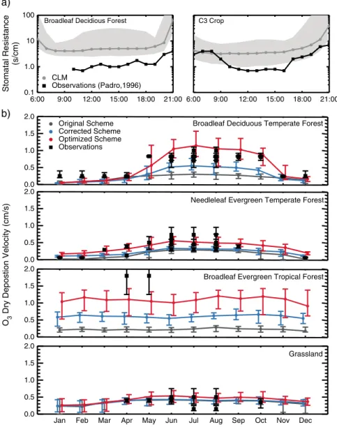
Figure 2. Comparison of modeled and observed (a) daytime stomatal resistance (Rs) and (b) midday O3dry
deposi-tion velocity (Vd).Rsdata show modeled median and minimum-maximum range (gray) and average from observations (black).Rsobservations are averages from measurements collected over a broadleaf deciduous forest in Ontario, Canada,
and a cotton field in Sacramento, California, during the summer (JJA) [Padro, 1996].Vdobservations (see Table 2) are
shown in black, and results from three simulations are shown in grey (Original), blue (Corrected), and red (Optimized), respectively. Symbols show the mean values; vertical bars represent the minimum-maximum range.
vegetation dependence (Corrected Scheme). O3dry deposition and surface concentrations are substan-tially affected by linking the dry deposition scheme to LAI, in particular over densely vegetated regions. For example, the eastern U.S. is dominated by broadleaf deciduous forests and summertime LAI is about 4.5 (Figure S1). Deposition velocities increase by 0.25 cm/s (80% increase) with the Corrected Scheme. This leads to a decrease of 12 ppb of surface O3over the region in summertime.
To examine the performance of the original and corrected dry deposition schemes, we compare modeled Rswith observations. We evaluate daytime Rsbecause direct uptake through the stomata pores is the
dom-inant O3removal process over vegetation; for most vegetation types, this uptake only occurs during the day as stomata are closed at night [e.g., Wesely, 1989; Lamaud et al., 2002; Wu et al., 2011]. Figure 2a dis-plays daytime Rsobservations based on long-term measurements gathered in a broadleaf deciduous forest in Ontario, Canada, and a cotton field in Sacramento, California, during the summertime extracted from
Padro [1996], Figure 2. We compare these observations to the simulated median Rs, and the minimum and
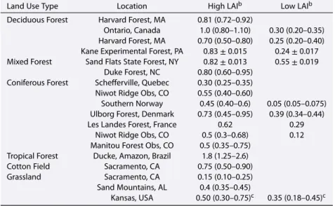
Table 2. A Review of Daytime O3Dry Deposition Velocities Over Main PFTsa
Land Use Type Location High LAIb Low LAIb Deciduous Forest Harvard Forest, MA 0.81 (0.72–0.92)
Ontario, Canada 1.0 (0.80–1.10) 0.30 (0.20–0.35) Harvard Forest, MA 0.70 (0.50–0.80) 0.25 (0.20–0.40) Kane Experimental Forest, PA 0.83±0.015 0.24±0.017 Mixed Forest Sand Flats State Forest, NY 0.82±0.013 0.55±0.019
Duke Forest, NC 0.80 (0.60–0.95) Coniferous Forest Schefferville, Quebec 0.30 (0.25–0.35) Niwot Ridge Obs, CO 0.55 (0.40–0.60)
Southern Norway 0.45 (0.40–0.6) 0.05 (0.05–0.075) Ulborg Forest, Denmark 0.73 (0.45–0.95) 0.39 (0.34–0.44) Les Landes Forest, France 0.62 0.29
Niwot Ridge Obs, CO 0.5 (0.3–0.68) 0.12 Manitou Forest Obs, CO 0.5 (0.35–0.75)
Tropical Forest Ducke, Amazon, Brazil 1.8 (1.25–2.6) Cotton Field Sacramento, CA 0.75 (0.50–0.90) Grassland Sacramento, CA 0.15 (0.10–0.25) Sand Mountains, AL 0.4 (0.35–0.45)
Kansas, USA 0.50 (0.30–0.75)c 0.35 (0.18–0.45)c aReported daytime (9:00–15:00 LST)V
das average (minimum-maximum), avg±SD or
average. Data extracted from Wu et al. [2011], Padro et al. [1991], Padro et al. [1992], Munger et al. [1996], Finkelstein et al. [2000], Kumar et al. [1983], Hole et al. [2004], Mikkelsen et al. [2000], Lamaud et al. [2002], Turnipseed et al. [2009], Park et al. [2014], Fan et al. [1990], Padro et al. [1994], Meyers et al. [1998], and Gao and Wesely [1995].
bHigh LAI are periods with active plant growth and large LAI and Low LAI are periods with no plant growth or/and snow cover (see text for further explanation).
cV
dfor 10:00–14:00.
temperate forests and C3 crops at those locations. The diurnal variability of Rsis mainly regulated by radia-tion, which controls stomatal opening. During the day, Rsdecreases rapidly and reaches a minimum around
local noon when stomata are fully open and vegetation photosynthesis activity is at a maximum [e.g.,
Wesely, 1989; Padro, 1996]. Observed daytime Rsvalues range from 0.7 to 6 s/cm in both PFTs, and noon
minima are 1 s/cm and 0.7 s/cm in the broadleaf deciduous temperate forest and cotton field, respectively. Similar daytime Rsvalues have been reported in other, however limited, studies. Finkelstein et al. [2000] measured daytime average Rsvalues of 2–6.4 s/cm over different broadleaf deciduous temperate trees;
Grantz et al. [1997] reported daytime O3Rsof 1.4–6.6 s/cm inferred from water vapor stomatal conductance
measurements in a cotton field. The Ball-Berry Rsscheme implemented in CESM captures the diurnal
vari-ability of observed Rs. However, the model substantially overestimates the Rsmagnitude by a factor of 5.
Lombardozzi et al. [2012] suggest that O3damage to plants (not included here) would further increase the
stomatal resistance; including this effect would exacerbate the model bias in stomatal resistance. Canopy parameters used to calculate Rsare not well constrained in CLM4, and that may contribute to the large
Rsvalues [Bonan et al., 2011]. It is also important to note that Rsis difficult to measure, and observations
are rather limited. Therefore, other sources of uncertainty may account for or contribute to the difference observed between the model and observations. However, it is unlikely that vegetation density is a major factor here. We find that a 50% increase in the LAI increases summertime midday Vdby about 20%, with a
concurrent decrease of 3 ppb in surface O3concentrations. Therefore, we use this initial model-observation comparison to optimize the Rsvalues implemented in our dry deposition scheme.
Figure 1c shows results from a simulation in which we reduce the Rsused in the dry deposition scheme by
a factor of 5 to match the observations shown in Figure 2a (Optimized Scheme). This Optimized Scheme also includes the updated vegetation dependence of the Corrected Scheme. The impact of the Optimized Scheme on the ozone simulation is substantial. For example, in the eastern U.S. dry deposition velocities are 0.5 cm/s (∼200%) larger than the Original Scheme, with a concurrent decrease of 20 ppb in surface O3 concentrations. We observe similar decreases in surface O3over dense vegetated regions in the tropical Southern Hemisphere (e.g., Amazon) where LAI is large (∼ 5) throughout the year.
Geophysical Research Letters
10.1002/2014GL059651
20 30 40 50 60 70 80 CASTNET (ppb) 20 30 40 50 60 70 80 Model (ppb) 20 30 40 50 60 70 80 EMEP (ppb) 20 30 40 50 60 70 80 Eastern US Europea)
b)
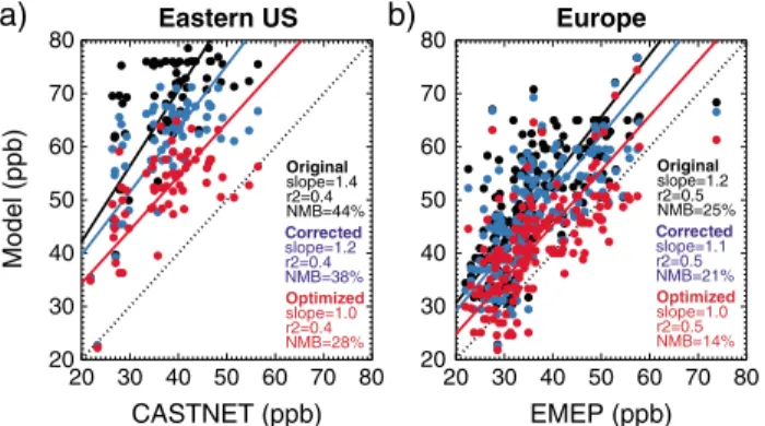
Figure 3. Scatterplots of simulated surface O3during the summer (JJA) with the Original Scheme (black), Corrected
Scheme (blue) and Optimized Scheme (red) versus observed long-term mean values at (a) individual Clean Air Status and Trends Network (CASTNET) sites (1995–2005) in eastern U.S. and (b) individual European Monitoring and Evaluation Programme (EMEP) sites (1990–2009) in Europe. Squared-correlation coefficients (r2), slope, and normalized mean biases (NMB) are shown in the inset. Reduced–major axis regression lines (solid) and the 1:1 lines (dash) are also shown. To further support the changes suggested by our Corrected and Optimized schemes, we compare simu-lated ozone dry deposition velocities with observations in Figure 2b. We show the seasonal variation of O3 Vdover four sites (Harvard Forest (MA, USA), Rocky Mountain National Park (CO, USA), the Amazon (Brazil),
and Kansas (USA)) representative of four major PFTs (broadleaf deciduous temperate forest, needleleaf ever-green temperate forest, broadleaf everever-green tropical forest, and grassland). We show the monthly average of midday (9:00–15:00 LST) Vdas well as the minimum and the maximum values simulated by CESM at these locations. Table 2 summarizes midday Vdfrom field observations reported in the literature over dif-ferent PFTs. We report midday Vdfor high LAI and low LAI periods to distinguish the effect of growth and vegetation density on the deposition velocity. We define “high LAI” as periods with active plant growth and large LAI and “low LAI” as periods with no plant growth or/and snow cover, as defined in each study. Figure 2b includes observations from four of these PFTs, shown as the average and minimum and maximum (or ± standard deviation (SD)) reported in each study for the duration of measurement period. The compar-ison of O3Vdobservations from a particular location with global CESM model output (1.9◦×2.5◦horizontal
resolution) may be biased because of heterogeneity within the grid box. However, we ensure that the grid box, from which the model data are extracted, is dominated by the PFT in which observations were col-lected. Figure 2b shows that the ozone dry deposition is generally underestimated (in some cases by more than a factor of two) in the Original Scheme and both our Corrected and Optimized schemes improve comparisons with observations. The dry deposition velocity is particularly sensitive to Rsunder densely
vegetated (high LAI) conditions. For example, the Optimized Scheme produces Vdvalues that are a factor of
two larger than the Corrected Scheme in deciduous forests during the summer and tropical forests through-out the year (∼1 cm/s versus 0.5 cm/s), whereas it remains nearly constant in all configurations in deciduous forests during the winter (∼0.1 cm/s) and grasslands (∼0.3 cm/s).
In broadleaf deciduous temperate forests, Vdis primarily controlled by the seasonal cycle of LAI (Figure S1)
[e.g., Finkelstein et al., 2000; Wu et al., 2011]. Observations show a pronounced seasonality in Vdwith larger
values from late spring to early fall (∼0.8 cm/s in summer versus 0.1 cm/s in winter; Table 2). It is clear that the original dry deposition scheme configuration has little skill in capturing the seasonal variability of Vd.
The new schemes dependent on LAI reproduce the seasonal cycle, with the Optimized Scheme capturing both the variability and the magnitude of the cycle. Similar results are found in needleleaf evergreen temperate forests, with a much less pronounced seasonality in the simulated and observed Vd.
In broadleaf evergreen tropical forests and grasslands, modeled and observed Vdshow little to no
season-ality. In these PFTs, where LAI remains nearly constant throughout the year [e.g., Turnipseed et al., 2009;
Gao and Wesely, 1995], Vdis mainly driven by environmental factors, such as temperature, humidity, light,
and the presence of snow. In broadleaf evergreen tropical forests, the Optimized Scheme improves the comparison with observed dry deposition velocities but is still biased low. It is important to note that Vd
observations over tropical regions are very scarce, and data shown are based on only one field campaign (Table 2). In grasslands, dry deposition is not very sensitive to vegetation as LAI is very low (<1; Figure S1), and all configurations reproduce the observed ozone dry deposition velocities.
Figure 3 shows how these changes to the simulation of dry deposition affect the comparison of simu-lated surface O3concentrations with observations during the summer. In this comparison, we focus on the eastern United States and Europe since these are regions with dense observational networks and where a consistent positive bias in simulated surface O3has previously been identified. Observations shown for the eastern U.S. and Europe are long-term means from the CASTNET and EMEP networks, respectively. As an example, we show the bias between model and observations with the original dry deposition scheme in Figure S2 (supporting information). Over the eastern U.S. (Figure 3a), the simulation of surface O3 concen-trations is positively biased with all dry deposition scheme configurations. However, including LAI in the dry deposition scheme significantly improves the simulation of surface O3. The Original Scheme has a mean positive bias of 30 ppb with respect to the observations, i.e., a 44% normalized mean bias (NMB), which is similar to that obtained for other periods studied with CESM [Lamarque et al., 2012], and is clearly outside of the range of climate variability in surface O3. This bias drops to 23 ppb (38% NMB) in the Corrected Scheme and to 14 ppb (28% NMB) in the Optimized Scheme. Over Europe (Figure 3b), all model configurations also tend to overestimate surface O3. However, both the Corrected Scheme and Optimized Scheme are substan-tially closer to observations (respectively, 5 and 10 ppb bias versus 13 ppb in the Original Scheme). A more detailed evaluation using ozone sondes and satellite and aircraft observations shows that the updates to the dry deposition scheme have a negligible effect on O3concentrations above 900 hPa, and away from regions and periods with dense vegetation, i.e., eastern U.S. and Europe during the summer and Southern Hemisphere tropical regions (S. Tilmes, National Center for Atmospheric Research (NCAR), personal com-munication, 2014). Therefore, while the simulation of surface ozone is dramatically impacted by the representation of vegetation phenology in the dry deposition scheme, the global tropospheric ozone bud-get is largely unaffected. In addition, our changes to the dry deposition scheme have little impact on the simulation of other species (e.g., SO4, NO2, and CO), which are less sensitive to dry deposition losses [e.g., Wesely, 1989].
3. Conclusions
Dry deposition represents an important physical mechanism controlling surface O3in CESM. Correcting the vegetation dependence and optimizing the stomatal resistance used in the dry deposition scheme in CESM leads to a substantial improvement in the simulation of surface O3over regions that are well known to have a positive bias (e.g., eastern U.S. and Europe). Thus, ozone biases reported in the literature [e.g., Murazaki and Hess, 2006; Lamarque et al., 2012] using the Original Scheme can, at least in part, be attributed to impor-tant oversimplifications in the implementation of the dry deposition scheme. Ensuring that models correctly link ozone deposition processes with vegetation and use accurate dry deposition schemes may be a first step toward improving surface O3simulations. However, our Optimized Scheme is based on limited obser-vational constraints, and additional globally distributed measurements of both stomatal resistance and dry deposition velocities could be used to improve this parameterization. Further work is also needed to fully understand the causes of the bias in the simulated stomatal resistance, and the impact that the scal-ing applied in our Optimized Scheme may have on the simulation of the hydrological and carbon cycle, via greater stomatal water loss and carbon uptake. Finally, including explicit links between vegetation param-eters and dry deposition is critical to the ability of Earth System Models to simulate surface O3response to future and past vegetation changes, as well as factors controlling changes in stomatal resistance, such as changes in CO2and drought stress. Thus, on-going investigation of the accuracy of such links must proceed concurrently with efforts to project changing global air quality.
References
Baldocchi, D. D., B. B. Hicks, and P. Camara (1987), A canopy stomatal resistance model for gaseous deposition to vegetated surfaces,
Atmos. Environ., 21(1), 91–101, doi:10.1016/0004-6981(87)90274-5.
Bonan, G. B., S. Levis, L. Kergoat, and K. W. Oleson (2002), Landscapes as patches of plant functional types: An integrating concept for climate and ecosystem models, Global Biogeochem. Cycles, 16(2), 1021, doi:10.1029/2000GB001360.
Bonan, G. B., P. J. Lawrence, K. W. Oleson, S. Levis, M. Jung, M. Reichstein, D. M. Lawrence, and S. C. Swenson (2011), Improving canopy processes in the Community Land Model version 4 (CLM4) using global flux fields empirically inferred from FLUXNET data, J. Geophys.
Res., 116, G02014, doi:10.1029/2010JG001593.
Collatz, G., J. Ball, C. Grivet, and J. A. Berry (1991), Physiological and environmental regulation of stomatal conductance, photosynthesis and transpiration: A model that includes a laminar boundary layer, Agric. For. Meteorol., 54(24), 107–136, doi:10.1016/0168-1923(91)90002-8.
Emmons, L. K., et al. (2010), Description and evaluation of the Model for Ozone and Related chemical Tracers, version 4 (MOZART-4),
Geosci. Model Dev., 3(1), 43–67, doi:10.5194/gmd-3-43-2010.
Acknowledgments
This work was supported by the U.S. National Park Service (grant H2370 094000/J2350103006), the U.S. National Science Foundation (AGS-1238109), and the JFSP (project ID 13-1-01-4). We thank Sam Levis (NCAR), Gordon Bonan (NCAR), Louisa Emmons (NCAR), J-F Lamarque (NCAR), and Bill Munger (Harvard) for helpful discussions and Simone Tilmes (NCAR) for running a full diagnostic on the CESM output. S.R.A. acknowledges support from the NCAR Advanced Study Program and NCAR Atmospheric Chemistry Division. The CESM project is supported by the National Science Foundation and the Office of Science (BER) of the US Department of Energy. Computing resources were provided by the Climate Simulation Laboratory at NCAR’s Computational and Information Systems Laboratory (CISL), sponsored by the National Science Foundation and other agencies. Any opinions, findings, and conclusions or recommendations expressed in this material are those of the author(s) and do not necessarily reflect the views of the National Science Foundation.
The Editor thanks two anonymous reviewers for their assistance in evaluating this paper.
Geophysical Research Letters
10.1002/2014GL059651
Fan, S.-M., S. C. Wofsy, P. S. Bakwin, D. J. Jacob, and D. R. Fitzjarrald (1990), Atmosphere-biosphere exchange of CO2and O3in the centralAmazon Forest, J. Geophys. Res., 95(D10), 16,851–16,864, doi:10.1029/JD095iD10p16851.
Finkelstein, P. L., T. G. Ellestad, J. F. Clarke, T. P. Meyers, D. B. Schwede, E. O. Hebert, and J. A. Neal (2000), Ozone and sulfur dioxide dry deposition to forests: Observations and model evaluation, J. Geophys. Res., 105(D12), 15,365–15,377, doi:10.1029/2000JD900185. Fiore, A. M., et al. (2009), Multimodel estimates of intercontinental source-receptor relationships for ozone pollution, J. Geophys. Res., 114,
D04301, doi:10.1029/2008JD010816.
Ganzeveld, L., L. Bouwman, E. Stehfest, D. P. van Vuuren, B. Eickhout, and J. Lelieveld (2010), Impact of future land use and land cover changes on atmospheric chemistry-climate interactions, J. Geophys. Res., 115, D23301, doi:10.1029/2010JD014041.
Gao, W., and M. Wesely (1995), Modeling gaseous dry deposition over regional scales with satellite observations: Model development,
Atmos. Environ., 29(6), 727–737, doi:10.1016/1352-2310(94)00284-R.
Grantz, D., X. Zhang, W. Massman, A. Delany, and J. Pederson (1997), Ozone deposition to a cotton (Gossypium hirsutum l.) field: Stomatal and surface wetness effects during the California Ozone Deposition Experiment, Agric. For. Meteorol., 85(12), 19–31, doi:10.1016/S0168-1923(96)02396-9.
Hole, L., A. Semb, and K. Tayseth (2004), Ozone deposition to a temperate coniferous forest in Norway; Gradient method measurements and comparison with the EMEP deposition module, Atmos. Environ., 38(15), 2217–2223, doi:10.1016/j.atmosenv.2003.11.042. Kumar, A., F. Chen, D. Niyogi, J. Alfieri, K. Manning, M. Ek, and K. Mitchell (1983), Using photosynthesis-based canopy resistance model
and new MODIS-based data to improve the presentation of vegetation transpiration in the Noah land surface model, Tech. Rep. J3.1. 22nd conference of hydrology, Am. Meteorol. Soc., New Orleans, La.
Lamarque, J.-F., et al. (2012), CAM-Chem: Description and evaluation of interactive atmospheric chemistry in the Community Earth System Model, Geosci. Model Dev., 5(2), 369–411, doi:10.5194/gmd-5-369-2012.
Lamaud, E., A. Carrara, Y. Brunet, A. Lopez, and A. Druilhet (2002), Ozone fluxes above and within a pine forest canopy in dry and wet conditions, Atmos. Environ., 36(1), 77–88, doi:10.1016/S1352-2310(01)00468-X.
Lapina, K., D. K. Henze, J. B. Milford, M. Huang, M. Lin, A. M. Fiore, G. Carmichael, G. G. Pfister, and K. Bowman (2014), Assess-ment of source contributions to seasonal vegetative exposure to ozone in the US, J. Geophys. Res. Atmos., 119, 324–340, doi:10.1002/2013JD020905.
Lombardozzi, D., J. Sparks, G. Bonan, and S. Levis (2012), Ozone exposure causes a decoupling of conductance and photosynthesis: Implications for the Ball-Berry stomatal conductance model, Oecologia, 169(3), 651–659, doi:10.1007/s00442-011-2242-3. Meyers, T. P., P. Finkelstein, J. Clarke, T. G. Ellestad, and P. F. Sims (1998), A multilayer model for inferring dry deposition using standard
meteorological measurements, J. Geophys. Res., 103(D17), 22,645–22,661, doi:10.1029/98JD01564.
Mikkelsen, T., H. Ro-Poulsen, K. Pilegaard, M. Hovmand, N. Jensen, C. Christensen, and P. Hummelshoej (2000), Ozone uptake by an evergreen forest canopy: Temporal variation and possible mechanisms, Environ. Pollut., 109(3), 423–429, doi:10.1016/S0269-7491(00)00045-2.
Munger, J. W., S. C. Wofsy, P. S. Bakwin, S.-M. Fan, M. L. Goulden, B. C. Daube, A. H. Goldstein, K. E. Moore, and D. R. Fitzjarrald (1996), Atmospheric deposition of reactive nitrogen oxides and ozone in a temperate deciduous forest and a subarctic woodland: 1. Measurements and mechanisms, J. Geophys. Res., 101(D7), 12,639–12,657, doi:10.1029/96JD00230.
Murazaki, K., and P. Hess (2006), How does climate change contribute to surface ozone change over the United States?, J. Geophys. Res.,
111, D05301, doi:10.1029/2005JD005873.
Neale, R. B., J. Richter, S. Park, P. H. Lauritzen, S. J. Vavrus, P. J. Rasch, and M. Zhang (2013), The mean climate of the community atmosphere model (CAM4) in forced SST and fully coupled experiments, J. Clim., 26, 5150–5168, doi:10.1175/JCLI-D-12-00236. Oleson, K. W., et al. (2010), Technical description of version 4.0 of the Community Land Model (CLM), Tech. Rep. Technical Note
NCAR/TN-478+STR, 257 pp. NCAR.
Olson, J. S., J. A. Watts, and L. J. Allison (1983), Carbon in live vegetation of major world ecosystems, Tech. Rep. ORNL-5862. Oak Ridge Natl. Lab., Oak Ridge, Tenn.
Padro, J. (1996), Summary of ozone dry deposition velocity measurements and model estimates over vineyard, cotton, grass and deciduous forest in summer, Atmos. Environ., 30(13), 2363–2369, doi:10.1016/1352-2310(95)00352-5.
Padro, J., G. den Hartog, and H. Neumann (1991), An investigation of the ADOM dry deposition module using summertime O3 measurements above a deciduous forest, Atmos. Environ., 25(8), 1689–1704, doi:10.1016/0960-1686(91)90027-5.
Padro, J., H. Neumann, and G. Hartog (1992), A wintertime comparison of modelled and observed dry deposition velocity of O3over a deciduous forest, in Air Pollution Modeling and Its Application IX, NATO Challenges of Modern Society, vol. 17, edited by H. Dop and G. Kallos, pp. 495–501, Springer, New York, doi:10.1007/978-1-4615-3052-749.
Padro, J., W. Massman, R. Shaw, A. Delany, and S. Oncley (1994), A comparison of some aerodynamic resistance methods using mea-surements over cotton and grass from the 1991 California ozone deposition experiment, Boundary Layer Meteorol., 71(4), 327–339, doi:10.1007/BF00712174.
Park, R. J., S. K. Hong, H.-A. Kwon, S. Kim, A. Guenther, J.-H. Woo, and C. P. Loughner (2014), An evaluation of O3dry deposition simulations in East Asia, Atmos. Chem. Phys. Discuss., 14(1), 919–951, doi:10.5194/acpd-14-919-2014.
Reidmiller, D. R., et al. (2009), The influence of foreign vs. North American emissions on surface ozone in the US, Atmos. Chem. Phys.,
9(14), 5027–5042, doi:10.5194/acp-9-5027-2009.
Sanderson, M. G., C. D. Jones, W. J. Collins, C. E. Johnson, and R. G. Derwent (2003), Effect of climate change on isoprene emissions and surface ozone levels, Geophys. Res. Lett., 30(18), 1936, doi:10.1029/2003GL017642.
Sanderson, M. G., W. J. Collins, D. L. Hemming, and R. A. Betts (2007), Stomatal conductance changes due to increasing carbon dioxide levels: Projected impact on surface ozone levels, Tellus B, 59(3), 404–411, doi:10.1111/j.1600-0889.2007.00277.x.
Sellers, P. J., S. O. Los, C. J. Tucker, C. O. Justice, D. A. Dazlich, G. J. Collatz, and D. A. Randall (1996), A revised land surface parameterization (SiB2) for atmospheric GCMS. Part II: The generation of global fields of terrestrial biophysical parameters from satellite data, J. Clim., 9, 706–737, doi:10.1175/1520-0442(1996)009<0706:ARLSPF>2.0.CO;2.
Turnipseed, A. A., S. P. Burns, D. J. Moore, J. Hu, A. B. Guenther, and R. K. Monson (2009), Controls over ozone deposition to a high elevation subalpine forest, Agric. For. Meteorol., 149(9), 1447–1459, doi:10.1016/j.agrformet.2009.04.001.
Wesely, M. (1989), Parameterization of surface resistances to gaseous dry deposition in regional-scale numerical models, Atmos. Environ.,
23(6), 1293–1304, doi:10.1016/0004-6981(89)90153-4.
Wild, O. (2007), Modelling the global tropospheric ozone budget: Exploring the variability in current models, Atmos. Chem. Phys., 7(10), 2643–2660, doi:10.5194/acp-7-2643-2007.
Wu, S., L. J. Mickley, D. J. Jacob, J. A. Logan, R. M. Yantosca, and D. Rind (2007), Why are there large differences between models in global budgets of tropospheric ozone?, J. Geophys. Res., 112, D05302, doi:10.1029/2006JD007801.
Wu, S., L. J. Mickley, J. O. Kaplan, and D. J. Jacob (2012), Impacts of changes in land use and land cover on atmospheric chemistry and air quality over the 21st century, Atmos. Chem. Phys., 12(3), 1597–1609, doi:10.5194/acp-12-1597-2012.
Wu, Z., et al. (2011), Evaluating the calculated dry deposition velocities of reactive nitrogen oxides and ozone from two community models over a temperate deciduous forest, Atmos. Environ., 45(16), 2663–2674, doi:10.1016/j.atmosenv.2011.02.063.
Zhang, L., J. R. Brook, and R. Vet (2002), On ozone dry deposition with emphasis on non-stomatal uptake and wet canopies, Atmos.