HAL Id: inria-00577223
https://hal.inria.fr/inria-00577223
Submitted on 12 Jan 2012
HAL is a multi-disciplinary open access
archive for the deposit and dissemination of
sci-entific research documents, whether they are
pub-lished or not. The documents may come from
teaching and research institutions in France or
abroad, or from public or private research centers.
L’archive ouverte pluridisciplinaire HAL, est
destinée au dépôt et à la diffusion de documents
scientifiques de niveau recherche, publiés ou non,
émanant des établissements d’enseignement et de
recherche français ou étrangers, des laboratoires
publics ou privés.
Copyright
Using host profiling to refine statistical application
identification
Mohamad Jaber, Roberto Cascella, Chadi Barakat
To cite this version:
Mohamad Jaber, Roberto Cascella, Chadi Barakat. Using host profiling to refine statistical
appli-cation identifiappli-cation. IEEE INFOCOM Mini-Conference, Mar 2012, Orlando, United States. pp.9,
�10.1109/INFCOM.2012.6195692�. �inria-00577223�
Using host profiling to refine statistical application
identification
Mohamad Jaber, Roberto G. Cascella and Chadi Barakat
INRIA - FranceEmail: {mohamad.jaber, roberto.cascella, chadi.barakat}@inria.fr
Abstract—The identification of Internet traffic applications is very important for ISPs and network administrators to protect their resources from unwanted traffic and prioritize some major applications. Statistical methods are preferred to port-based ones and deep packet inspection since they don’t rely on the port number, which can change dynamically, and they also work for encrypted traffic. These methods combine the statistical analysis of the application packet flow parameters, such as packet size and inter-packet time, with machine learning techniques. Other successful approaches rely on the way the hosts communicate and their traffic patterns to identify applications.
In this paper, we propose a new online method for traffic classi-fication that combines the statistical and host-based approaches in order to construct a robust and precise method for early Internet traffic identification. We use the packet size as the main feature for the classification and we benefit from the traffic profile of the host (i.e. which application and how much) to refine the classification and decide in favor of this or that application. The host profile is then updated online based on the result of the classification of previous flows originated by or addressed to the same host. We evaluate our method on real traces using several applications. The results show that leveraging the traffic pattern of the host ameliorates the performance of statistical methods. They also prove the capacity of our solution to derive profiles for the traffic of Internet hosts and to identify the services they provide.
I. INTRODUCTION
The identification of Internet traffic applications is very important for ISPs and network administrators to protect their resources from unwanted traffic and prioritize some major applications. On the one hand, this allows to treat flows in a different way based on their quality of service requirements and allocate more resources based on the type of traffic. On the other hand, it can serve for security reasons by blocking unwanted traffic and limiting worm spreading or looking closely at those users who run non legacy applications.
The identification of Internet traffic becomes more and more complex because of mechanisms that bypass firewalls or mask the type of application. Historically, the recognition was done by using the port number. Yet, some applications use dynamic non-standard port numbers; this is typically the case of telephony over IP. Other applications hide themselves using standard ports stolen from other applications, such as port 80, to pass firewalls. These ports are usually given by the end host and thus they can be easily changed.
Current techniques of ”Deep Packet Inspection” (DPI) [1], [2] make it possible to go further in the identification of the applications but they require a complete and costly exploration
of the payload of the packets. This induces an important load to inspect packets and create the signatures, which requires updates with the appearance of new applications. Moreover, when packets are encrypted, the recognition fails.
The statistical techniques [3]–[7] seem to be today an interesting alternative. They allow to recognize and to classify the applications according to their statistical signatures. These signatures can be volumes (number of bytes) per connection, connection durations, rates, inter-packet delays, packet sizes, and direction. Most of these techniques require a machine learning phase to perform the classification of connections (or flows) into applications. In [4], McGregor et al. show the utility of using clustering algorithms for the identification of the traffic. They propose to use an unsupervised machine learning, called auto class, and the following statistical criteria: packet size, inter-arrival time, byte count, and connection duration. In [3], Moore et al. use a Naive Bayesian classifier for TCP traffic, and try to find the best set of statistical criteria. In [5], Bernaille et al. test three clustering algorithms (K-Means, Gaussian mixture model, and the Spectral clustering); the input features to assign flows to applications are the size and the direction of the first four packets jointly used. In [6], Crotti et al. classify Internet traffic by using the packet size and inter-packet time. In our previous work [7], we develop a method to iteratively classify Internet traffic while using the size and the direction of the packets.
The common feature of statistical methods is that they classify every flow independently of each other using the pattern of its packets (size, time, and direction). Indeed, they don’t correlate the information across flows having as end points the same hosts, thus not using any information about the traffic pattern of the originating host or the type of services that run on the destined server. Some recent works have focused on this aspects by considering the role of the hosts [8], [9] or the relations of the traffic between end points [10], [11]. Our solution differs from these studies since we only rely on the information that a monitor collects passively from the packet flows and we do not require any information related to the groups of communicating hosts, such as a graphlet [8].
We believe that the classification of previous flows sharing the same IP address either as source and/or destination is important to refine the classification of future flows. For instance, a host browsing the Web is more prone to open several consecutive HTTP connections. A machine hosting a POP3 mail server is very likely to receive POP3 flows. In
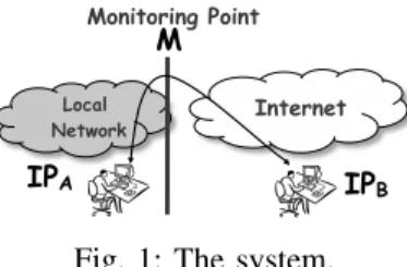
2 Internet IPA IPB Local Network Monitoring Point M
Fig. 1: The system.
general, hosts have profiles for their flows either because of the behavior of users or the services run on them, and these profiles can help in the identification of flows in which they are implied. Our idea is to build the traffic profile of hosts, based on the result of the classification of previous flows, and then use this information to refine the classification of subsequent flows. On one hand these profiles help in flow classification and on the other hand they point to the behavior of the users behind them and on the network services they deploy.
In this paper we propose a novel two-step approach to affect flows to applications. In the initial classification phase, we use an iterative statistical technique to classify Internet traffic, based solely on the flow statistical features. The results give an initial classification. In the second phase, we use the traffic profile of the host to refine the classification and, then, to update the host profile based on the classification results. Our contribution can be summarized as follows. First, we define the host profile and we determine the host-based probability that a flow is of a given application. We then develop a new method that relies on the result of the classification of flows from the same host to determine the profiles of hosts; these profiles are later used as an initial guess before the classification of future flows. The host profiles are updated after each classification using an exponential weighted moving average filter to absorb any transient behavior; the way the profile accounts for past classified flows depends on a discounting parameter, which can be decided by the network administrator.
Another contribution refers to the validation methodology. We use two real traces to test our method and to show how to characterize the traffic pattern of each host in the traces. For the purpose of having a complete evaluation of our technique, these traces are aggregated to account for more applications, thus reducing the bias given by a small subset of applications in each separate trace. The results on the aggregate trace indeed confirm that leveraging the host profile improves the classification of Internet flows.
The rest of the paper is organized as follows. Section II introduces the host profiling and discusses the related work. Section III explains our classification method. Section IV and Section V describe the traces and the evaluation results, respectively. Section VI concludes the paper.
II. HOST TRAFFIC PROFILE
In this section we introduce our definition of the traffic profile of a host and we present the benefits of using this information to refine the classification of Internet applications while discussing the related work. The methodology herein described is general and can be integrated to any flow classi-fication method transparently.
Without loss of generality we consider a monitoring point at the edge of the network, located in the ISP network, as shown in Fig. 1. The monitor passively captures the flows between any two hosts; a flow consists of the packets with the same 5-tuple (IP source and destination, port source and destination, IP protocol). For each flow there are one host located inside the ISP network (IPA in Fig. 1) and a destination host
downstream the monitoring point (IPB in Fig. 1); we don’t
assign any specific role to these two hosts, IPA and IPB,
which can act as client or server during a session indifferently. The monitor inspects the packets of each flow and extracts statistical information, or the signature of the flow, such as packet size, inter-packet time, direction of the packet, etc. This statistical signature is then used to assign the flow to the application that matches it. In this section we focus on the profile of the host, while the definition of this signature and classification procedure are detailed in Section III.
The traffic profile of a host consists of the type of appli-cations which run at the host and generate Internet traffic. This profile is determined at the monitor, which stores the results of the classification of the Internet traffic of the hosts. Practically, the monitor can be interested to log the traffic of the hosts inside the ISP network, and/or only those of interest from outside the ISP network. In addition, the monitor might decide to store information about some IP addresses that run dedicated services since this can help with the classification of Internet flows. The traffic profile, so computed, gives an indication of the preferred applications that run at the host and of the type of traffic the ISP would expect from the host. The motivation behind our solution is the recent studies on residential networks, which give an insight of user traffic profile [12], [13]. An interesting outcome of these studies is that users tend to hardly mix P2P and HTTP (Web streaming), which are the most predominant applications [12].
In this section, we first discuss how a monitor computes the probability that a flow of packets between two hosts is of a certain application solely using the traffic patterns of these hosts. Then, we discuss how the monitor computes and updates the host profile.
A. Host based probability of a flow
The host based probability of a flow is defined as the probability that a flow is generated by an application computed based on the traffic profile of the hosts, i.e., source and destination. If we consider that the two traffic profiles of the source and destination of a flow are different and that these are used jointly in the computation, then, this probability consists of those cases when the predictions computed with the partial info of each host are in accordance.
Let F denote a function that associates a packet flow between a source S and destination D to an application A(i), with 1 ≤ i ≤ NA and NA being the number of monitored
applications. Thus, FS and FD are the functions that assign
the flow to the application AS and AD based solely on the
traffic profile of the source and destination respectively. Then, let P (FS = AS|S) (or P (FD = AD|D)) be the probability
that, given the host traffic profile of the source, the flow is of an application AS(or ADfor the destination). The probability
P (F = A(i)) that the flow is of application A(i) can then be computed as follows:
P (F = A(i)) = P ((FS = A(i)S) ∩ (FD= A(i)D)|AS = AD)
= P (FS = A(i)|S) ∗ P (FD= A(i)|D) PNA j=1P (F = A(j)|S ∩ D) (1) = P (FS = A(i)|S) ∗ P (FD= A(i)|D) PNA j=1P (FS = A(j)|S) ∗ P (FD= A(j)|D)
Eq. (1) shows that we compute the probability by con-sidering the cases when the prediction for each host is in accordance by considering the traffic profiles of S and D separately, i.e., we know that the same application is running on both sides. Equation (1) also holds when the monitor only records the traffic profile of one of the two hosts. In fact, if we assume a uniform probability for the other host, e.g., P (FD = AD|D) = N1A, then, equation (1) simplifies to
P (F = A(i)) = P (FS = A(i)|S).
B. Host profile definition and update
The monitor computes and updates the profile of the hosts. After capturing and classifying the flows, two traffic profiles are generated for each host. Indeed, each host can be the source or the destination of the Internet flows. The former is the host that sends the first packet of the flow, as we discuss in Section II, while the latter is the one that receives it. We keep these two profiles separated since they characterize the role of the host when being the source or the destination. For example, a host can send HTTP requests to a server or receive SSH requests when is running a local SSH server. In the rest of the section, we consider a generic host and we focus on the computation of the source profile for this host; the destination profile is defined in the same way.
Let S denote the generic source host of a flow and FS the
function that maps the flow to an application by only lever-aging the traffic profile of the source. The monitor computes the host profile by using previous classified flows. The profile, denoted P (A|S) in this case, is defined as the prior distribution for the flows in the space A, which defines the applications A(i), 1 ≤ i ≤ NA. If the monitor has not any information
about previous traffic of a host, then, the monitor considers a uniform prior distribution. The prior distribution is updated after each classification of a new collected flow.
The profile update works as follow. Let P(n−1)(A(i)|S)
be the prior probability for application A(i) computed from the past (n − 1) flows. The monitor affects the n − th flow to the application A(i) with probability P (FS = A(i)|S)
for each application. Then, the posterior probability for each application is computed as follows:
P(n)(A(i)|S) = λ ∗ P(n−1)(A(i)|S)+
+ (1 − λ) ∗ P (FS(n) = A(i)|S). (2)
P (FS(n) = A(i)|S) is the result of the classification of
flow n and λ, 0 ≤ λ ≤ 1, represents the discounting factor
for past classifications. When λ is close to 0, the profile is computed by associating a higher weight to the most recent flows. When λ is close to 1 the profile is calculated over a longer period, which means that the profile is determined in equal measure by all previous classified flows. When λ = 1 the profile corresponds to the initial prior distribution, which in our case assigns a uniform probability to all applications. The best choice of λ depends on the traffic pattern of the host and on the performance of the classifier. We will discuss more about λ in Section V.
The traffic profile of the same host while being the desti-nation, it is computed in a similar way by considering only the flows destined to this host. It is worth noticing that the monitor needs to store the two prior distributions if it want to fully determine the profile of the host. In practice, given the limitation of the resources, the monitor can decide to track and store profiles for a subset of hosts (source and/or destinations) and use simple uniform profiles for the other hosts. In this case, the method will also work well but with less accuracy since the more hosts we track better the classification of Internet flows is for these hosts. Table I shows an example of the source and destination profiles of a host.
TABLE I: Example of a traffic profile of a host
Applications: FTP HTTP POP3 SMTP SSH
Source: 0.02 0.76 0 0.2 0.02
Destination: 0.22 0 0.1 0.23 0.45
C. Related work
The problem of profiling the Internet hosts has been recently introduced in the area of Internet traffic classification. Most solutions focus on the behavior of the end-user, for instance, to determine what is the mix of used applications, the preferred destinations, the pattern of port usage [12], [14]. The first studies in the area of Internet traffic classification focus on determining the role of the host [8], [9]. BLINC [8] is a solution for Internet traffic identification that focuses on the source and destination of the flows to determine the host behavior, which is studied across three levels: social to account for the host popularity and communities of hosts (groups of communicating hosts), functional to identify the functional role of a host (offered services, used services), and protocol patterns of the host. In [9], Trestian et al. characterize the role and type of traffic of an end-point by collecting publicly available information on the Web, based on the IP address of the host. The main difference, which is also the strength, of our approach consists of only considering the flows sent and received by the monitored hosts and in crossing the information between flows of the same host so as to build profiles and have a better classification. We construct and leverage the profiles of the communicating hosts on the fly without requiring the traffic monitor to maintain a detailed history of their interactions.
Other works focus on the application classes of the Internet traffic between end-points to refine the classification of Internet flows [10], [11]. They analyze the graph of connections between end-points and leverage the different patterns of
4
the traffic connections to refine the classification. [11] also shows how this method can be applied in the network core, when not all the flows of the end points are sampled. The main difference with our approach is that we do not use collective traffic statistics but we are interested in reducing at the minimum the burden at the monitoring node, which can rely solely on information locally available.
The novelty of our approach consists of using the traffic pattern of end hosts to predict future flows that involve the same hosts. It is worth noticing that our definition of the host profile leverages information already available at the monitor, which is passively captured, and does not need the analysis of the relations between flows of different hosts.
III. METHODDESCRIPTION
Our purpose for the classification of Internet traffic is to detect online which flow belongs to which application. We use a statistical and iterative method that computes the probability that packets are generated by an application. We have defined and used this method to classify Internet traffic based on the size of the packets in [7]. The method allows an iterative classification of the flows for each packet size independently and uses more packet sizes for the identification of an application until the classifier reaches a predefined threshold. Each flow corresponds to a sequence of N packets independently of their direction.
In this section we first propose an overview of our method and then we detail how the method uses the host profile to refine the classification. The method consists of three main phases: the model building phase, the classification phase, and the application probability or labeling phase. The the traffic profile of the host is used in the labeling phase.
A. Model building and classification phases
We use K-Means as supervised machine learning algorithm to partition the input in a predefined number of clusters. Given the number of clusters NC, K-Means assigns each input
feature to a cluster so as to minimize the Euclidean distance of each input from the centroid of the cluster.
P ktk denotes the packet size, i.e., the observations, and
for each packet size we train separately K-Means to obtain different set of classes. Thus, the packet sizes of position k have their own independent training, and the model used for testing its determined by the position of a packet in a flow. The input feature corresponds to the size of the packet associated with a sign that represents the direction of the packet. A positive sign corresponds to a packet from the source to the destination. In the learning algorithm, every class is affected by all applications with different probabilities proportional to the number of flows from each application present in the class. Hence, each class defines the probability that the elements within this class are generated by the applications.
The model building phase consists of constructing these sets of classes (clusters) by using a training data set, described in Section IV. Let denote C(j) the clusters, where 1 ≤ j ≤ NC
and NCis the number of clusters. Then, the per-class
probabil-ity P (C(j)|A(i)), knowing the application A(i) is computed for all the clusters during this learning phase. We build a separate model, i.e., set of classes, for every packet size noted by P ktk and we use these classes for the classification phase.
The classification phase consists of using the classes defined in the learning phase to test and assign the Internet flows to a class. The test is performed by computing the Euclidean distance between the input feature from the k − th packet in the flow and the centroid of each class determined for the k-th packet size. We affect the point to the closest class. The test is repeated for all the packet sizes of a flow iteratively until we reach a predefined threshold. The classification result is the probability that the packet size P ktk identifies an application.
B. Application probability or labeling phase
In the labeling phase we assign a flow to an application knowing the result of the classification and the host based probability computed from the profiles of the source and destination, as discussed in Section II. We combine iteratively the results of the classification for each single packet size and we calculate the probability (P (A(i)) that a flow belongs to an application A(i) given the prediction from the host profiles and the classification results of the first N packet sizes (i.e., class C(j(1)) for the first packet size, class C(j(2)) for the second packet size and so on).
P (A(i)) = P (A(i)|Result ∩ P (F = A(i))) = P (F = A(i)) ∗ QN k=1P (C(j(k))|A(i)) PNA i=1[P (F = A(i)) ∗ QN k=1P (C(j(k))|(A(i))] (3) P (F = A(i)) is the probability that a flow between a source and a destination comes from application A(i) based on their traffic profiles and it is calculated in Eq. (1). P (C(j(k))|A(i)) is the probability that P ktk of a flow belongs to the class
C(i) knowing the application A(i). NA is the total number
of applications. We call P (A(i)) the assignment probability. It combines the result of the classification, obtained with the K-Means clustering method, and the result of the classification that one would have if solely the pattern of the hosts is used to predict the type of application for the next flow.
This assignment probability is computed when the monitor captures each packet of the same flow. This means that the classification of the application starts with the first packet. This iterative process stops when the highest assignment probability is above a predetermined threshold or the maximum allowed number of tests is reached. The threshold is seen as a way to leave the classification phase earlier when one is sure about the type of application. The monitor updates the profiles of the hosts that are of interest, i.e., the source and/or the destination, once the labeling phase ends. The host profiles are updated as described in Section II-B.
IV. TRACEDESCRIPTION
In our analysis we use two real traces, see Table II for de-tails. The two traces have been collected at the edge gateway of
TABLE II: Traces Description
Source and Date Application training testing
Brescia University HTTP 8000 17,263 April 2006 [6] SMTP 8000 19,835 POP3 8000 19,935 Brescia University HTTP 500 30422 Fall 2009 [15] HTTPS 500 3608 EDONKEY 500 3702 BITTORENT 500 3608
the Brescia University’s campus network. The first trace, noted trace I [6], was collected during April 2006 and the second trace, noted trace II [15], was collected on three consecutive working days during fall 2009. Every trace consists of two sets, a training set and a testing set; the type of applications associated with each flow is determined with a deep packet inspection method.
In the learning phase we use the training set, which consists of an equal number of flows per application to ensure that there is no bias in our learning. The application flows in the training set are only used to construct the classes in K-Means. The testing set is used to evaluate how well our iterative method behaves in identifying the application.
V. EXPERIMENTAL RESULTS
In this section we present the evaluation results of our method when the traffic profile of the hosts is used to refine the classification. We compare these results with a classification that uses the same iterative classification technique but does not leverage the profile of the end host. It is worth noticing that the training is the same for both cases, since the training phase is used only for the supervised machine learning algorithm to create the signature of each application; thus, not including any information about the traffic profile of the host. The host profile is automatically computed during the testing phase. We initially consider a uniform prior distribution for the source and destination profiles of an unknown host. Then, we update the profiles once flows of this host are collected. The following results only show the case of a monitor that computes the profile of the hosts located inside the ISP domain, since its interest is on the the network usage of its ISP customers. The monitor might also decide to maintain the information about popular Internet servers and also leverage these profiles to improve the Internet traffic identification, as we discuss in Section II. For example, if one tracks the facebook server, he can directly identify flows without the need for more analysis. We use the traces described in Section IV and we profile the hosts with the same IP prefix, i.e., those inside the Brescia campus. For addresses outside the campus, we have counted an average of 10 flows per IP address, therefore there is not a significant number of flows per IP to compute the profile.
The flows are all TCP connections and the hosts within the campus are the source of the flow. The metrics used for the evaluation are:
• False Positive (FP) rateis the percentage of flows of other
applications classified as belonging to an application I.
• True Positive (TP) rate is the percentage of flows of application I correctly classified.
0.8 0.85 0.9 0.95 1 1 2 3 4 5 6 7 8 9 10 Total Precision Number of Packets 20 classes 50 classes 80 classes 200 classes 400 classes
Fig. 2: Total precision of an Internet traffic classification with a different number of class as input to K-Means (Trace I).
0.8 0.85 0.9 0.95 1 1 2 3 4 5 6 7 8 9 10 Total Precision Number of Packets lambda=0.1 lambda=0.5 lambda=0.9 lambda=1
Fig. 3: Total precision versus the number of packets (Trace I).
• Precisionis the ratio of flows that are correctly assigned to an application, T P/(T P + F P ). The overall precision is the weighted average over all applications given the number of flows per application.
We run the test for all the available packet sizes to test its significance as a feature for identifying applications. We set the number of clusters equal to 200 for K-Means. We have tested the supervised machine learning algorithm with different number of clusters and 200 (see Figure 2) has shown the best results: it allows to group the features in small clusters and to account for possible noise in the observations; it gives a significant number of samples in each cluster to infer its characteristics. It is also a good tradeoff between precision and speed of classification.
A. Classification results
In this section we discuss the performance of the classi-fication method when the host profile is used to refine the probability that a flow is of a given application type.
1) Total Precision: Fig. 3 and 4 plot the total precision for trace I and trace II respectively versus the number of packets used for the classification. Our method classifies a flow at each packet iteratively, as we discuss in Section III. The different lines in the plot correspond to the precision of the classifier when different values of the discounting factor λ are used. The value of λ determines the weight assigned to the last classification results. When λ = 0.1, the most recent classification results characterize the profile of the host. When λ = 0.9, the host profile is computed over a longer period. The value of λ = 1 means that a uniform probability is associated to each application, thus, the host profile is not used, as we discuss in Section II-B. The results show that the precision of the classifier improves considerably when the profile of the hosts is used to decide in favor of this or that application, especially for the first four packets.
For Trace I, we can observe in Fig. 3 that a value of λ = 0.9 gives the best performance for the classifier. We obtain a precision of 96% already after two packets reaching
6 0.9 0.92 0.94 0.96 0.98 1 1 2 3 4 5 6 7 8 9 10 Total Precision Number of Packets lambda=0.1 lambda=0.5 lambda=0.9 lambda=1
Fig. 4: Total precision versus the number of packets (Trace II)
0.3 0.4 0.5 0.6 0.7 0.8 0.9 1 1 2 3 4 5 6 7 8 9 10 True positive Number of Packets lambda=0.1 lambda=0.5 lambda=0.9 lambda=1
(a) TP ratio - POP3
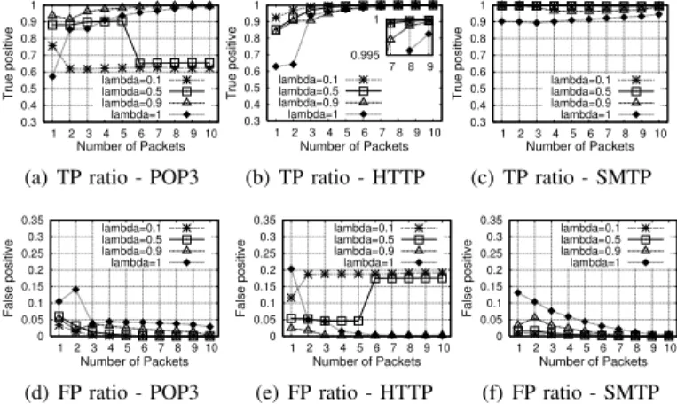
0.3 0.4 0.5 0.6 0.7 0.8 0.9 1 1 2 3 4 5 6 7 8 9 10 True positive Number of Packets lambda=0.1 lambda=0.5 lambda=0.9 lambda=1 0.995 1 7 8 9 (b) TP ratio - HTTP 0.3 0.4 0.5 0.6 0.7 0.8 0.9 1 1 2 3 4 5 6 7 8 9 10 True positive Number of Packets lambda=0.1 lambda=0.5 lambda=0.9 lambda=1 (c) TP ratio - SMTP 0 0.05 0.1 0.15 0.2 0.25 0.3 0.35 1 2 3 4 5 6 7 8 9 10 False positive Number of Packets lambda=0.1 lambda=0.5 lambda=0.9 lambda=1 (d) FP ratio - POP3 0 0.05 0.1 0.15 0.2 0.25 0.3 0.35 1 2 3 4 5 6 7 8 9 10 False positive Number of Packets lambda=0.1 lambda=0.5 lambda=0.9 lambda=1 (e) FP ratio - HTTP 0 0.05 0.1 0.15 0.2 0.25 0.3 0.35 1 2 3 4 5 6 7 8 9 10 False positive Number of Packets lambda=0.1 lambda=0.5 lambda=0.9 lambda=1 (f) FP ratio - SMTP Fig. 5: Classification results for Trace I.
99.9% after 10 packets. For λ = 0.1 and 0.5 the classifier predicts with less accuracy the applications with a precision that reaches 95%. With this value of λ the classifier is more sensitive to recent flows. Thus, the classification is less accurate if the host has a uniform traffic behavior over all applications. For this trace we have that a big number of flows belong to two different applications and are generated uniformly by the same host, and that the method classifies the applications with less precision for small values of λ. If one does not leverage the host profile (λ = 1) the precision of the classifier is quite low (89%) after two packets, but it keep increasing when more packets are analyzed (98% after 10 packets). This result confirms that the host profile helps in deciding about a flow when little information can be extracted from the statistical analysis of the flow.
For Trace II and for all the selections of λ, we have better performance compared to the classification without host profile information (λ = 1). Indeed, Fig. 4 shows that if the host profile is used, then the precision already increases after the first packet, and then converges to 99% after the fifth packet in all cases. These results show that the use of the host information increases the precision (in comparison of the classification without host information) of the classifier especially for the first four packets. We can conclude that the profile of the host gives an early characterization of a flow because of the traffic pattern of the host. For instance, we can consider that a host browsing the Web has high probability to have a sequence of HTTP connections. Thus, the use of information about the host profile helps our statistical method. 2) True Positive: A more detailed analysis is needed to con-firm the advantage of the host profile to refine the classification of Internet flows. Fig. 5 shows the True (TP) and False (FP)
Positive ratios as a function of the number of packets used for the classification of trace I. We discuss the TP ratio in this section and the FP ratio in the following one. Let consider first POP3 flows and the case of λ = 0.9, which gives the best total precision, see Fig. 3. The TP ratio (Fig. 5(a)) ranges from 97%, with the first packet, to 99%, with ten packets. This shows an important improvement compared to the case when the host information is not used. In this case the initial TP ratio is 56%, reaching 90% after four packets and 99% after ten packets. When λ = 0.5 and 0.1 the TP ratio drops significantly after 6 and 2 packets respectively. This means that the classifier fails to identify correctly POP3 flows as they are assigned to other applications. This behavior will be confirmed with the analysis of the False Positive ratio, since it sheds lights about the output application of our classification method. The fact that this only happens for these small values of λ means that we have some hosts that interleave POP3 flows with others of different applications.
Fig. 5(b) and Fig. 5(c) plot the True Positive (TP) ratio for HTTP and SMTP as a function of the number of packets respectively. Fig. 5(b) shows that the TP ratio increases for all the values of λ, even when we do not use any host information. The classifier has better performance with λ = 0.1, which means that there are consecutive HTTP flows in general. We can notice clearly the importance of using the host informa-tion. This gives a very high accuracy even when the first packet is used only. From Fig. 5(c) it is interesting to notice that the TP ratio is 99% for any number of packets of SMTP when we use the profile of the host to refine the classification. The fact that the precision is very high for all values of λ means that the SMTP traffic is predominant in some hosts, confirming the benefit of profiling hosts.
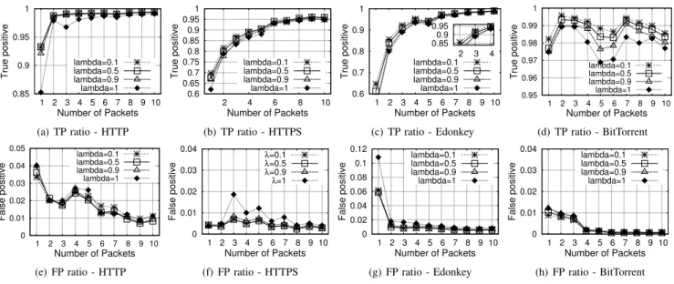
Fig. 6 plots the results for Trace II with a different set of applications. We can clearly observe that for all the values of λ we have better performance compared to the classification without host profile information (λ = 1). The True Positive ratio keeps increasing when more packets are used for the classification. For all the applications we can observe that we have better performance when we use a small value for λ, which means that we don’t have a lot of changes in the traffic pattern of these hosts. In any case, λ = 0.9, which shows to improve the classification for Trace I, gives an important improvement also for this trace (Trace II). For HTTP (Fig. 6(a)), we obtain an excellent precision by using the host profile with a TP ratio always above 99% after the first packet, compared to a 99% after the fifth packet for λ = 1. The classification of HTTPS flows (Fig. 6(b)) has always a good precision for all the values of λ even for λ = 1, converging to 94% approximately after six packets.
In case of P2P applications, such as Edonkey and BitTor-rent our two-step classification method also achieves good performance. The True Positive ratio for the Edonkey flows (Fig. 6(c)) is 95% after the fifth packet and converges to 99% after ten packets for all values of λ. The BitTorrent flows (Fig. 6(d)) can be better identified by using the first packets with the True Positive ratio above 98% for all valued of λ.
0.95 0.96 0.97 0.98 0.99 1 1 2 3 4 5 6 7 8 9 10 True positive Number of Packets lambda=0.1 lambda=0.5 lambda=0.9 lambda=1 (a) TP ratio - HTTP 0.8 0.85 0.9 0.95 1 2 4 6 8 10 True positive Number of Packets lambda=0.1 lambda=0.5 lambda=0.9 lambda=1 (b) TP ratio - HTTPS 0.6 0.7 0.8 0.9 1 1 2 3 4 5 6 7 8 9 10 True positive Number of Packets lambda=0.1 lambda=0.5 lambda=0.9 lambda=1 0.85 0.9 0.95 2 3 4 (c) TP ratio - Edonkey 0.95 0.96 0.97 0.98 0.99 1 1 2 3 4 5 6 7 8 9 10 True positive Number of Packets lambda=0.1 lambda=0.5 lambda=0.9 lambda=1 (d) TP ratio - BitTorrent 0 0.01 0.02 0.03 0.04 1 2 3 4 5 6 7 8 9 10 False positive Number of Packets lambda=0.1 lambda=0.5 lambda=0.9 lambda=1 (e) FP ratio - HTTP 0 0.01 0.02 0.03 0.04 1 2 3 4 5 6 7 8 9 10 False positive Number of Packets lambda=0.1 lambda=0.5 lambda=0.9 lambda=1 (f) FP ratio - HTTPS 0 0.01 0.02 0.03 0.04 1 2 3 4 5 6 7 8 9 10 False positive Number of Packets lambda=0.1 lambda=0.5 lambda=0.9 lambda=1 (g) FP ratio - Edonkey 0 0.005 0.01 0.015 0.02 1 2 3 4 5 6 7 8 9 10 False positive Number of Packets lambda=0.1 lambda=0.5 lambda=0.9 lambda=1 (h) FP ratio - BitTorrent Fig. 6: Classification results for Trace II (They are shown with different scales).
Indeed, the distribution of the size of the first packets is very different compared to the one of other applications, so that the packet size is very effective to classify BitTorrent traffic. Better performance can be achieved when the host profile is used. This result is supported by the analysis of the traffic behavior of the Internet users of P2P applications [12], as we discuss in Section II.
We can conclude from the results of the True Positive ratio that the host information increases the performance of the classification especially for the first four packets.
3) False Positive: Finally we discuss the results of the False Positive ratio for Trace I and Trace II. For Trace I (Fig. 5(d)) we can immediately notice that the percentage of misclassified flows of other applications, assigned to POP3, drops significantly after 4 packets, with slightly better perfor-mance (3% against 5%) when the host profile is used to refine the classification. The drop of True Positive ratio, shown in Fig. 5(a), is explained by analysing the False Positive ratio of HTTP traffic (Fig. 5(e)). Indeed, most of the POP3 flows that have not been detected are classified as HTTP traffic. This is clear for values of λ = 0.1 and λ = 0.5. For the higher values of λ the FP ratio drops to 0% after the fifth packet. Fig. 5(f) shows that the classification for most of the SMTP traffic is indeed correct when the classification of recent flows has more weight. When λ = 0.9, the classifier labels other flows as SMTP, which means that some hosts have SMTP flows interleaved with other applications.
The False Positive ratio for Trace II is shown in Fig. 6 and also in this case the performance of the classification method with host profile information improves the performance for all applications. The error in classifying flows in the case of False Positives is always below 4%. This is something expected from the analysis of the True Positive results of all applications. B. Importance of the discounting factor λ
The classification results have validated our two-step clas-sification technique. The performance depends on the tuning
0.9 0.92 0.94 0.96 0.98 1 0 0.1 0.2 0.3 0.4 0.5 0.6 0.7 0.8 0.9 1 Total Precision Lambda 4 Packets 7 Packets 10 Packets
Fig. 7: Total precision as a function of λ (Trace I). of the right value of λ, which accounts for the importance of the past flows in the host profile. In this section we discuss more in detail this parameter and provide some guidelines by discussing classification results for Trace I.
Fig. 7 plots the total precision as a function of λ. The discounting factor λ determines how previous flows are con-sidered for the classification of a new one. We recall that for λ close to 1 the host profile is computed over a longer period and previous flows have similar weights. The opposite case is when λ is close to 0. In Fig. 7, a precision above 90% for all values of λ proves that our iterative method is effective in classifying the applications. We also notice that when few packets are used for the classification (4 in the plot), the profile of the user helps for an early detection of the Internet traffic. In this case, the machine learning algorithm does not have much information about a flow and it associates to applications comparable classification probabilities. Thus, for these first packets the profile of the host has higher influence on the output of the classification.
The choice of a correct λ is important to improve the classification even if more information is available. From Fig. 7, we can notice that high values perform better for the total precision because the classifier is less sensitive to sudden traffic burst of a single application. For instance, let consider the case of Web browsing. It generates many HTTP flows since most of the servers open parallel connections to improve the performance or because the user navigates from one page to the next one. However, other programs run in background, such as e-mail clients, thus, opening new connections when needed. High values of λ also accounts for the few flows
8 0 0.2 0.4 0.6 0.8 1 1 10 100 1000 CDF # of consecutive flows POP3 HTTP SMTP
(a) Consecutive application flows
0 0.2 0.4 0.6 0.8 1 1 10 100 1000 CDF
# of flows of other applications POP3 HTTP SMTP
(b) Other application flows Fig. 8: CDF of number of consecutive application flows and of other applications for an IP address inside the ISP network. of other applications than HTTP. We conclude that the host profile prediction is more accurate because we associate a probability to the application of the next flow based on the fraction of past traffic of the same application.
C. Traffic pattern of a host
In Trace I, described in Table II, we have identified different types of hosts. In particular, there are some hosts within the Brescia campus that are dedicated to single services and other hosts that use all the three applications. In this section, we analyze in details the traffic of the latter type of hosts and we determine their profile. This will shed light on the importance of λ for the identification of the Internet traffic. As example we analyze one host generating a big number of flows, denoted for simplicity IP 1. The total number of flows generated by IP 1 is 14, 151, subdivided as follows: 7, 101 HTTP flows, 7, 014 POP3 flows, and only 35 SMTP flows.
Fig. 8(a) plots the cumulative distribution (CDF) of consec-utive flows of the same type of application in a semi-log scale. Since there are only 35 SMTP flows, most of these flows are isolated so that there are only sequences of 1 to 3 consecutive flows. Almost 60% of the POP3 traffic consists of a single flow; the rest of the POP3 traffic consists of few larger bursts and the largest one consists of almost 700 flows. The number of small HTTP consecutive flows is 10% of the total number of HTTP traffic and 80% of the bursts consist of less than 100 flows. This is to a typical browsing activity of a user, who surfs from one Web site to another by following hyper-links.
The fact that the medium size burst of HTTP traffic get interleaved with POP3 has evident impact on our profiling method when we use a small value of λ. In particular, since there are more consecutive HTTP flows than POP3, the host based classification with a small value of λ is more sensitive to the presence of a new burst. Moreover, the analysis (not shown in the paper) of the packet size distribution of POP3 and HTTP flows shows many similarities for certain packet numbers making the host profile decide the classification.
To conclude the characterization of the profile, Fig. 8(b) plots the cumulative distribution (CDF) of flows of other applications that separate two flows of the same application. There are more than 60% of HTTP flow bursts separated by only 1 flow of another application and 80% of HTTP flow bursts separated by less than 10 consecutive flows, while POP3 has 20% and 60% of bursts respectively. The small bursts of other applications between two HTTP flows justify the high value of False Positives ratio (see Fig. 5(e)). In general, this is more pronounced with small values of λ, making a high value
0.8 0.85 0.9 0.95 1 1 2 3 4 5 6 7 8 9 10 Total Precision Number of Packets lambda=0.1 lambda=0.5 lambda=0.9 lambda=1
Fig. 10: Total precision After trace aggregation (Trace II). of λ the best choice to leverage the host profile optimally. D. Trace aggregation
In this section we present a new technique to construct a trace to stress the robustness our classification scheme with host profile information and obtain a complete evaluation of its applicability in more complex scenarios. We are aware that the two traces (see Table II) used for the evaluation sample partially the space of possible applications which are not present in both traces. Thus, the complexity of the training of the supervised machine learning is limited to the number of applications in each trace and our classification results can be biased by the fact that the training phase is done only for these few applications.
We propose an aggregate model for the traces to train K-Means on a larger set of applications. We do a joint training for the entire set of applications available in the traces, presented in Section IV. To these sets, we add the applications from another trace collected at the edge of the INRIA Sophia Antipolis Network; we separately collect the traffic from servers dedicated to unique applications hosted at the INRIA Network [7]. Moreover, we use other applications present in Trace II [15] that were initially excluded since not enough flows are available to have a significant representation of an application. The applications that we use are: Skype, BitTorrent, Edonkey, HTTP, and HTTPS from Trace II [15]; SMTP and POP3 from Trace I [6]; SSH, FTP, and IMAP from the INRIA trace [7]. We use 8, 000 flows for each application and in case the number of available flows is not sufficient we replicate the existing flows to have a balanced number. The reason of using many flows is to train the K-Means algorithms properly and have a significant number of flows in each cluster; we use 200 clusters for the training. It is worth noticing that we are interesting in using the statistical information in each flow and understand how our two-step iterative mechanism is efficient in classifying application flows.
In the following we test Trace II and we present the classifi-cation results while using the aggregate model for training. We cannot test our method on the aggregate trace since we cannot validate the use of the host profile. We expect a decrease of performance since the model is trained to recognize other applications as well.
Fig. 10 shows the total precision of the classification. We can see clearly that the precision is still very good, even after the use of the aggregate trace. The aggregate model leads to slightly lower accuracy when compared to using the separate model learned from trace II (see Figure 4 for comparison), but with a precision that still converges to 98% after the sixth
0.85 0.9 0.95 1 1 2 3 4 5 6 7 8 9 10 True positive Number of Packets lambda=0.1 lambda=0.5 lambda=0.9 lambda=1 (a) TP ratio - HTTP 0.6 0.65 0.7 0.75 0.8 0.85 0.9 0.95 1 2 4 6 8 10 True positive Number of Packets lambda=0.1 lambda=0.5 lambda=0.9 lambda=1 (b) TP ratio - HTTPS 0.6 0.7 0.8 0.9 1 1 2 3 4 5 6 7 8 9 10 True positive Number of Packets lambda=0.1 lambda=0.5 lambda=0.9 lambda=1 0.85 0.9 0.95 2 3 4 (c) TP ratio - Edonkey 0.95 0.96 0.97 0.98 0.99 1 1 2 3 4 5 6 7 8 9 10 True positive Number of Packets lambda=0.1 lambda=0.5 lambda=0.9 lambda=1 (d) TP ratio - BitTorrent 0 0.01 0.02 0.03 0.04 0.05 1 2 3 4 5 6 7 8 9 10 False positive Number of Packets lambda=0.1 lambda=0.5 lambda=0.9 lambda=1 (e) FP ratio - HTTP 0 0.01 0.02 0.03 0.04 1 2 3 4 5 6 7 8 9 10 False positive Number of Packets λ=0.1 λ=0.5 λ=0.9 λ=1 (f) FP ratio - HTTPS 0 0.02 0.04 0.06 0.08 0.1 0.12 1 2 3 4 5 6 7 8 9 10 False positive Number of Packets lambda=0.1 lambda=0.5 lambda=0.9 lambda=1 (g) FP ratio - Edonkey 0 0.01 0.02 0.03 0.04 1 2 3 4 5 6 7 8 9 10 False positive Number of Packets lambda=0.1 lambda=0.5 lambda=0.9 lambda=1 (h) FP ratio - BitTorrent Fig. 9: Classification results after trace aggregation (They are shown with different scales).
packet for all values of λ. In all cases the classifier performs better when the host profile is used than without (λ = 1).
Finally we compare the True and False Positive ratios (see Fig. 9) for this last experiment with those shown in Fig. 6. As discussed above, the classifier detects correctly less flows, but the performance are really encouraging. In particular, we are interested to test the efficacy of using the host profile to refine the classification and to understand if our classification method can be generally applied. The TP ratio is very high for all the values of λ. For HTTP flows (Fig. 9(a)) this is 85% for λ = 1 and around 94% for the other values of λ; the TP ratio reaches approximately 97% after four packets for all the values of λ. There is also a decrease of performance, compared to the separate learning model, for HTTPS flows (Fig. 9(b)). The TP ratio reaches 90% after the forth packet, valued obtained already at the second packet for the separate learning (Fig. 6(b)). Fig. 9(c) and Fig.9(d) show that Edonkey and BitTorrent traffic is still well classified with the aggregate trace. As for the False Positive ratio (Fig. 9(e-h)), we can observe a similar decrease in performance, but the results are really encouraging since they show that the method is robust even when the complexity in the training increases, i.e., more applications are analyzed. From all these results we can confirm our claims about the useful use of the host information to refine the classification of Internet traffic flows.
VI. CONCLUSION
In this paper we present our new method for Internet traffic identification that combines the statistical and host-based approaches. The statistical parameters that we use are the size and direction of the first N packets. The novelty of our approach consists in leveraging the host profile to refine the classification. First we define the profile of the host and how it is updated. Then we show how the profiles of the source and destination hosts are used to assign a prediction probability to the new flow.
We evaluate our solution on two real traces and on a third trace obtained from their aggregation to reduce the bias in
the results given by a small subset of applications. We profile the hosts and we test our method for different values of the discounting factor λ, which defines how the profile accounts for past flows. The results show a great improvement for the classification of applications when the host profile is used. In particular, the classifier reaches a precision of 98% after using 10 packets for the classification. We discuss the optimal choice of λ and show that a high value, i.e., 0.9, gives better performance. Finally, we characterize the host profile and show the distribution of the flows, i.e., the traffic pattern of a representative host.
REFERENCES
[1] A. Moore and K. Papagiannaki, “Toward the accurate identification of network applications,” in PAM, October 2005.
[2] S. Sen, O. Spatscheck, and D. Wang, “Accurate, scalable in-network identification of p2p traffic using application signatures,” in WWW 2004 Conference, Philadelphia, USA, May 2004.
[3] A. Moore and D. Zuev, “Internet traffic classification using bayesian analysis techniques,” in ACM Sigmetrics, 2005.
[4] A. Mcgregor, M. Hall, P. Lorier, and J. Brunskill, “Flow clustering using machine learning techniques,” in PAM, 2004, pp. 205–214.
[5] L. Bernaille, R. Teixeira, and K. Salamatian, “Early application identi-fication,” in ADETTI/ISCTE CoNEXT Conference, December 2006. [6] M. Crotti, M. Dusi, F. Gringoli, and L. Salgarelli, “Traffic classification
through simple statistical fingerprinting,” in ACM-Sigcomm Computer Communication Review, vol. 37, January 2007, pp. 5 –16.
[7] M. Jaber and C. Barakat, “Enhancing application identification by means of sequential testing,” in NETWORKING, Aachen, Germany, 2009. [8] T. Karagiannis, K. Papagiannaki, and M. Faloutsos, “Blinc: Multilevel
traffic classification in the dark,” in SIGCOMM, New York, USA, 2005. [9] I. Trestian, S. Ranjan, A. Kuzmanovi, and A. Nucci, “Unconstrained endpoint profiling (googling the internet),” in ACM SIGCOMM, 2008. [10] Y. Jin, N. Duffield, P. Haffner, S. Sen, and Z.-L. Zhang, “Inferring
applications at the network layer using collective traffic statistics,” in the 22nd International Teletraffic Congress (ITC 22), 2010.
[11] M. Iliofotou, B. Gallagher, T. Eliassi-Rad, G. Xie, and M. Faloutsos, “Profiling-by-association: a resilient traffic profiling solution for the internet backbone,” in ACM Co-NEXT, 2010.
[12] M. Pietrzyk, L. Plissonneau, G. Urvoy-Keller, and T. En-Najjary, “On profiling residential customers,” in TMA, Vienna, Austria, 2011. [13] G. Maier, A. Feldmann, V. Paxson, and M. Allman, “On dominant
characteristics of residential broadband internet traffic,” in IMC, 2009. [14] T. Karagiannis, K. Papagiannaki, N. Taft, and M. Faloutsos, “Profiling
the end host,” in PAM, Louvain-la-Neuve, Belgium, 2007. [15] T. II, “Brescia university,” http://www.ing.unibs.it/ntw/tools/traces/.